ABSTRACT
ZENG, KAIYUE. Uncertainty Analysis Framework for the Multi-Physics Light Water Reactor Simulation. (Under the direction of Jason Hou.)
In recent years, the demand to provide best estimate predictions with confidence bounds is increasing for the nuclear reactor performance and safety analysis. As a result, the best-estimate plus uncertainty method (BEPU) has been approved by US NRC as an alternative approach to the conventional conservative methods for nuclear reactor safety evaluation. Input uncertainties from multi-physics domains will be considered, including neutron-kinetic parameters (NK), fuel modeling (FM) and thermal-hydraulics (TH) model-ing parameters. The goal of this work is to develop a framework for consistent uncertainty analysis of light water reactor modeling, with special consideration for the correlations between multi-physics input parameters.
In this work, a consistent uncertainty analysis methodology is proposed to represent the correlations between input parameters involve the usage of the global variance-covariance matrix (VCM) covering the NK few-group constants, FM and TH parameters. The sampling approach is used in constructing the global VCM. A number of samples are generated by independently sample fundamental input uncertainties (e.g. the fuel-cladding gap size), and samples of input parameters from three different physics domains can be obtained by performing lattice calculations, fuel modeling or thermal-hydraulics modeling. Each sample which combines input parameters from NK, FM and TH domains is consistent as they can be corresponded into the same sample of fuel-cladding gap size. A global VCM covering the input parameters from three different physics domains can then be generated from these consistent samples. The consistent uncertainty input parameters can be generated with sampling approach through Cholesky decomposition of the global VCM and Latin Hypercube Sampling method, and passed into the core multi-physics simulations. Therefore, the proposed framework can be incorporated into the conventional two-step light water reactor simulations for uncertainty analysis purposes.
© Copyright 2020 by Kaiyue Zeng
Uncertainty Analysis Framework for the Multi-Physics Light Water Reactor Simulation
by Kaiyue Zeng
A dissertation submitted to the Graduate Faculty of North Carolina State University
in partial fulfillment of the requirements for the Degree of
Doctor of Philosophy
Nuclear Engineering
Raleigh, North Carolina 2020
APPROVED BY:
Kostadin N. Ivanov Maria Avramova
Ralph C. Smith Jason Hou
DEDICATION
BIOGRAPHY
ACKNOWLEDGEMENTS
TABLE OF CONTENTS
LIST OF TABLES . . . vii
LIST OF FIGURES. . . viii
Chapter 1 INTRODUCTION. . . 1
1.1 Best Estimated Plus Uncertainty Approach . . . 1
1.2 Thesis Outline . . . 9
Chapter 2 DEVELOPMENT OF THE CONSISTENT UNCERTAINTY PROPAGATION METHODOLOGY. . . 10
2.1 Consistent Uncertainty Propagation for Two-Step Core Simulation . . . 12
2.2 Quantification of Confidence Intervals . . . 15
Chapter 3 INVESTIGATION OF CORRELATIONS BETWEEN DIFFERENT PHYSICS DOMAINS . . . 18
3.1 Multi-physics Model of the PWR Mini-Core . . . 19
3.2 Events Description . . . 23
3.3 Verification of VCM Generation . . . 23
3.4 Correlation of Input Parameters . . . 29
3.4.1 NK-TH Correlation Study . . . 32
3.4.2 NK-FM Correlation Study . . . 34
3.4.3 NK-FM-TH Correlation Study . . . 36
3.5 Summary . . . 37
Chapter 4 CONSISTENT UNCERTAINTY ANALYSIS OF THE TMI-1 REACTOR CORE 38 4.1 TMI-1 Reactor Core . . . 39
4.2 Numerical Test Cases . . . 39
4.3 Multi-Physics PWR Core Model . . . 41
4.4 Uncertainty Analysis of PWR Steady State Simulation . . . 42
4.5 Uncertainty Analysis of PWR Transient Simulation . . . 50
4.6 Uncertainty Analysis of PWR Cycle Depletion Simulation . . . 56
4.7 Summary . . . 58
Chapter 5 CONCLUSIONS AND FUTURE WORK . . . 59
5.1 Conclusions . . . 59
5.2 Future Work . . . 61
BIBLIOGRAPHY . . . 63
APPENDIX . . . 66
LIST OF TABLES
Table 3.1 Summary of core output responses comparing case 1 and case 2. . . 30 Table 3.2 Summary of the geometrical manufacturing uncertainties
consid-ered for PWR mini-core problem. . . 30 Table 3.3 Impact of the correlated and uncorrelated input uncertainties on
core outputs by taking into account NK-TH correlations. . . 35 Table 3.4 Impact of the correlated and uncorrelated input uncertainties on
core outputs by taken into account NK-FM correlations. . . 36 Table 3.5 Impact of the correlated and uncorrelated input uncertainties on
core outputs by taken into account NK-TH correlations. . . 37 Table 4.1 Core Physics Parameters at Nominal State. . . 43 Table 4.2 Summary of the geometrical manufacturing uncertainties
consid-ered for TMI-1 large-scale core problem. . . 44 Table 4.3 Summary of the geometrical manufacturing uncertainties
consid-ered for TMI-1 Reactor Core Steady State Simulation. . . 46 Table 4.4 A2and correspondingp−v a l u e s for power peaking factors at
vari-ous core states. . . 47 Table 4.5 Summary of uncertainty quantification on selected core
parame-ters at steady state simulations (numbers given in mean±relative standard deviation). . . 51 Table 4.6 Summary of uncertainty quantification for TMI-1 REA transient
sim-ulations (numbers given in mean+ [95t h/95% tolerance limit - mean]). 55
LIST OF FIGURES
Figure 1.1 Concept of BEPU approach and the benefit of BEPU analysis
com-pared to conservative analysis[9]. . . 3
Figure 1.2 Multi-physics multi-scale uncertainty quantification, with uncer-tainty originated from boundary condition (B.C.), modeling assump-tion, geometrical uncertainty and data uncertainty. . . 4
Figure 1.3 Strategy for uncertainty propagation from single physics to multi-physics simulations[12]. . . 6
Figure 1.4 Input uncertain parameters together with their fundamental sources of uncertainty. . . 8
Figure 2.1 Structure of the global variance-covariance matrix (VCM). . . 11
Figure 2.2 PWR core consistent uncertainty quantification with the stochastic sampling method. . . 12
Figure 2.3 Confidence intervals corresponding to different sample size. . . 17
Figure 3.1 PWR mini-core radial layout. . . 20
Figure 3.2 Conventional two-step LWR simulation approach. . . 21
Figure 3.3 Heat conduction (HtStr) and thermal-hydraulics (TH) model, axial NK-FM-TH mapping. . . 21
Figure 3.4 Cross section parameterization for fuel assemblies with control rod. 22 Figure 3.5 Correlation matrix of few-group constants. . . 24
Figure 3.6 Correlation matrix for PWR mini-core problem. . . 25
Figure 3.7 Distributions of original data (left), inverse transform sampling of CDF (mid.), and comparison of the distributions between original data and re-sampling data. . . 27
Figure 3.8 Running sample mean and uncertainty of the critical boron con-centration at case 1 (left) and case 2 (right). . . 27
Figure 3.9 Radial power distributions with associated uncertainties correspond-ing to case 1 (left) and case 2 (right). . . 28
Figure 3.10 Time evolution of core reactivity, total core power, and peak fuel temperatures under case 1 (left) and case 2 (right) configurations. . 29
Figure 3.11 Time evolution of core reactivity, total core power, and peak fuel temperatures under case 1 (left) and case 2 (right) configurations. . 33
Figure 3.12 Running sample mean and uncertainty of the critical boron con-centration at correlated case (left) and uncorrelated case (right). . . . 33
Figure 3.13 Radial power distributions with associated uncertainties correspond-ing at correlated case (left) and uncorrelated case (right). . . 34
Figure 3.14 Time evolution of peak fuel temperatures under at correlated case (left) and uncorrelated case (right) configurations. . . 34
Figure 4.1 TMI-1 quarter core configuration. . . 40
Figure 4.2 One Dimensional Channel model: TRACE TH, HTSTR models, and TH-HTSTR-NK mapping. . . 42
Figure 4.3 Correlation matrix of few-group constants,Hg a p,Dh,Ax andPw. . . 43
Figure 4.4 Running meanke f f for HFP at BOC. . . 45
Figure 4.5 Running meanke f f for HFP at EOC. . . 45
Figure 4.6 Frequency histogram of core key axial power peaking factors at HFP EOC state. . . 47
Figure 4.7 Core axial power under HFP BOC and HFP EOC steady states. . . 48
Figure 4.8 Radial power distribution at BOC . . . 49
Figure 4.9 Radial power distribution at EOC. . . 50
Figure 4.10 Core net reactivity during transient, initiated from HFP at BOC. . . . 52
Figure 4.11 Core net reactivity during transient, initiated from HFP at EOC. . . . 53
Figure 4.12 Normalized core power during transient, initiated from critical HFP at BOC. . . 53
Figure 4.13 Normalized core power during transient, initiated from critical HFP at EOC. . . 54
Figure 4.14 Peak fuel temperature during transient, initiated from HFP at BOC. 54 Figure 4.15 Peak fuel temperature during transient, initiated from HFP at EOC. 55 Figure 4.16 Core Burnup Distribution and Relative Error at EOC. . . 56
Figure 4.17 Burnups at EOC with Associated Uncertainties with consideration of NK-FM-TH correlations. . . 57
Figure 4.18 Burnups at EOC with Associated Uncertainties without considera-tion of NK-FM-TH correlaconsidera-tions. . . 57
Figure A.1 Axial TH-HTSTR-NK Mapping(a), 1-D Channel Model (b), 3-D Carte-sian Model (c). . . 70
CHAPTER
1
INTRODUCTION
1.1
Best Estimated Plus Uncertainty Approach
has grown interests in the application of best estimate plus uncertainty methodology in nuclear engineering problem. A series of workshops and benchmarks were launched by OECD NEA.
Figure 1.1 illustrates the benefit of using BEPU method compared to the traditional conservative method[8]. The safety limits such as peak cladding temperature were set up in a way that exceeding the limit would result in damage of the safety barrier. The actual margin could be computed as the distance between the real value and the safety limit. The acceptance criterion for reactor licensing purpose is usually determine by assigning some margins to the safety limits. In the conservative approach, the calculated conservative value is calculated following the guideline proposed in[9]by assigning margins to input parameters and assumptions. Therefore, the calculated conservative value is close to the ac-ceptance criterion. The BEPU approach, calculates a more realistic prediction, and provides associated uncertainty bounds. The distance of the 95t hupper bound of uncertainty to the
acceptance criterion is then taken as the BEPU margin. The BEPU approach is believed to yield larger margins compared to the conservative margin because no conservative hypotheses were made during the calculation, and therefore produce a more economic reactor design.
In order to establish the accuracy and confidence for best estimate codes, the uncer-tainty in reactor modelling must be quantified. In recent years, the demand to provide best estimate predictions with confidence bounds is increasing in the areas of nuclear research, industry, safety and regulation[10]. The uncertainty analysis has been regarded as a significant part in nuclear reactor design and analysis. Consequently, the Organization for Economic Cooperation and Development (OECD) Nuclear Energy Agency (NEA) has been developing an international benchmark for the uncertainty analysis in modelling of light water reactors (LWR-UAM) since 2006 for the examination of uncertainty quantifica-tion and propagaquantifica-tion methodologies for various modelling and simulaquantifica-tion code systems
Figure 1.1Concept of BEPU approach and the benefit of BEPU analysis compared to conserva-tive analysis[9].
forward the development, assessment, and integration of the comprehensive uncertainty quantification methods in best estimate multi-physics coupled simulations of LWRs during normal and transient conditions[12].
As shown in Figure 1.2, a series of reference systems and scenarios are defined with complete sets of input specifications and experimental data. The benchmark is being carried out in three phases with increasing modelling complexity, while each phase are further subdivided into multiple exercises[12]:
• Phase I (neutronics phase):
Figure 1.2Multi-physics multi-scale uncertainty quantification, with uncertainty originated from boundary condition (B.C.), modeling assumption, geometrical uncertainty and data uncertainty.
– Exercise I-2 (Lattice physics): Calculation of the few-group macroscopic cross-sections with associated uncertainties.
– Exercise I-3 (Core physics): Core steady state standalone neutronics calculations with associated uncertainties.
• Phase II (core phase):
– Exercise II-1 (Fuel modelling): Modelling of fuel thermal properties with associ-ated uncertainties.
– Exercise II-2 (Time dependent neutronics): Neutron kinetics and fuel depletion standalone performance with associated uncertainties.
– Exercise II-3 (Bundle thermal-hydraulics): Thermal-hydraulics fuel bundle per-formance with associated uncertainties.
– Exercise III-1 (Core multi-physics): Couple neutronics/thermal-hydraulics core simulation with associated uncertainties. This exercise includes coupled steady state, coupled depletion, and transient simulations with propagation of uncer-tainties from multi-physics domains including neutronics, fuel modelling and thermal-hydraulics.
– Exercise III-2 (System thermal-hydraulics): Calculation of the thermal-hydraulics system performance with associated uncertainties.
– Exercise III-3 (Coupled core-system): Coupled neutronics kinetics thermal-hydraulic core/thermal-hydraulic system performance.
– Exercise III-4: Comparison of best estimate plus uncertainty (BEPU) vs. Conser-vative Calculations.
The current approach for uncertainty propagation from three single physics domains to multi-physics uncertainty quantification is depicted in Figure 1.3. The uncertainties of different input parameters are calculated with considering the modelling uncertainties, ge-ometry uncertainties, uncertainties related to boundary condition and measurement data. The output parameters from single physics are then passed into multi-physics simulation with nominal value and associated uncertainty bounds.
Figure 1.3Strategy for uncertainty propagation from single physics to multi-physics simulations
[12].
of the uncertainties in Phase I have been summarized in[15]. Three reactor systems in-cluding the Peach Bottom Unit 2 BWR, Three Mile Island Unit 1 PWR, and VVER-1000 Kozloduy-6/Kalinin-3 have been studied. The methods of rigorous nuclear data uncertainty propagation have been widely investigated in multi-scale simulations including pin cell, assembly lattice and standalone core neutronics.
six-group kinetic parameters (Exercise II-2) were investigated and reported in[17]using a sampling-based method, and the capability of quantifying uncertainty from delayed neu-trons data would be available in the future release of SCALE code package. The uncertainty quantification of TMI-1 subchannel thermal-hydraulics was investigated in[16]. A sensitiv-ity analysis was performed to eliminate input parameters that have minimal influence on the quantities of interest, and the final thermal-hydraulic fuel bundle performance were reported with associated uncertainties (Exercise II-3). Various output quantities from multi-ple physics domains have been evaluated in Phase II and are treated as input uncertainties for reactor core multi-physics simulation (Exercise III-1), as discussed in[18]. Commissariat à l’Energie Atomique (CEA) studied a PWR mini-core, and performed uncertainty analysis in a control rod ejection accident. Separate studies with different level of multi-physics coupling were first conducted, and the input uncertainties were finally propagated to the core transient through the APOLLO3-FLICA4-ALCYONE coupling code framework[19].
uncertainties of input parameters from neutronics and fuel modelling domains.
Figure 1.4Input uncertain parameters together with their fundamental sources of uncertainty.
As a result, there is a need to propose an uncertainty analysis method for consistently propagating uncertainty in multi-physics LWR simulations. In this work we propose a framework that includes the following features:
1. it could be incorporated into the conventional light water reactor multi-physics simulation.
2. it should include uncertainties from three major physics domains.
ters must be quantified and propagated consistently.
4. it should be able to provide best-estimate predictions with uncertainty bounds and associated confidence levels.
1.2
Thesis Outline
In Chapter 2 a literature review of the statistical approach adopted for uncertainty analysis is performed. The Cholesky Decomposition is explained in detail. The methodology for multi-physics uncertainty propagation with consideration of the correlations between input uncertain parameters is presented in Chapter 2. The Anderson-Darling normality test is also described and the method of establishing the confidence intervals with certain confidence level is presented.
Chapter 3 focuses on the demonstration of the proposed consistent uncertainty propa-gation framework through the application of the method in a PWR mini-core problem. The multi-physics core steady state and control rod ejection transient are simulated and the out-put responses are evaluated with associated uncertainties. The impact of the correlations of input parameters on the uncertainties of core output responses is evaluated.
Chapter 4 presents the application of the framework on the Three Mile Island Unit # 1 (TMI-1) reactor core. The uncertainties of core output responses are evaluated by propagat-ing input uncertainties with and without the consideration of correlations between input parameters. Three types of problems related to Exercise III-1 of the LWR-UAM benchmark are studied, namely steady state calculation, control rod ejection accident, and cycle deple-tion analysis. The core simuladeple-tion results are reported with associated uncertain confidence bounds.
CHAPTER
2
DEVELOPMENT OF THE CONSISTENT
UNCERTAINTY PROPAGATION
METHODOLOGY
The approach for LWR simulation that is widely used in the industrial community is the two-step approach, which involves the generation of neutronic few-group constants as the first step, and the multi-physics core simulation as the second step. Code predictions are uncertain due to several sources of uncertainty, including neutron-kinetic (NK), fuel modeling (FM) and thermal-hydraulics (TH) parameters.
correlation between parameters from different physics domains on uncertainty analysis, a global variance-covariance matrix (VCM) needs to be constructed. As shown in Figure 2.1, the VCM consists of four regions. Region 1 represents the variance-covariance information of NK few-group constants, while region 2 corresponds to the TH or FM parameters. Region 3 and region 4 are symmetric and reflect the covariance between parameters from different physics domains. The VCM can be further sampled to generate correlated realizations of parameters, and the uncertainties of reactor core quantities of interest can be quantified using a stochastic sampling approach.
Figure 2.1Structure of the global variance-covariance matrix (VCM).
2.1
Consistent Uncertainty Propagation for Two-Step Core
Simulation
The stochastic sampling method is used on the two stages of the reactor core simulation, namely, the transport lattice and nodal core calculations, to propagate the uncertainties from nuclear data, fuel modelling and thermal-hydraulic parameters to output responses
[21]. The uncertain input variable vectorXfor nodal core simulation includes few-group constantsΣ, fuel modeling parametersγf and thermal-hydraulic parametersγt h, as shown in Eq. 2.1.
X = [Σ, γf, γt h] (2.1)
Figure 2.2PWR core consistent uncertainty quantification with the stochastic sampling method.
kandK are the index and the total number of realizations, respectively.
Xk = [Σk, γkf, γkt h]; k=1, 2, ...,K (2.2)
The correlations between input variables of[Σ,γf,γt h]can be evaluated, by tracing
back the uncertainties into the same uncertain source as illustrated in Figure 1.4. As shown in Figure 2.2, the uncertainties ofXcan be traced back into original multi-group nuclear dataσ, modeling and geometrical uncertaintiesρ, whose correlation has been evaluated (e.g., nuclear data VCM) or can be reasonably assumed as independent variable (e.g. fuel pellet outer surface and cladding thickness). Since the correlations are well known, a direct sampling procedure can be performed for generating realizations. These realizations can then be passed into lattice physics code and other modelling tools to generateXk.
With the abovementioned procedure, the consistency between different variables inside
[Σ,γf,γt h]can be maintained. The correlation information is carried in various realizations ofXk. Based on these realizations a global VCM can be estimated:
Cx=
V a r(Σ) C o v(Σ,γf) C o v(Σ,γt h) C o v(γf,Σ) V a r(γf) C o v(γt h,γt h) C o v(γt h,γf) C o v(γt h,γf) V a r(γt h)
(2.3)
where the diagonal terms are the variance and off-diagonal terms are covariances. By definition, the variance and covariance of variable x and y can be statistically estimated from a dataset ofK random realizations as:
V a r(x) = 1 K −1
K X
1
xk−x¯2 (2.4)
C o v(x) = 1 K −1
K X
1
xk−x¯ yk−y¯ (2.5)
the correlated realizationsxk. Withxk as input and the core multi-physics computational
model, the reactor core output responseRcan be evaluated as a function ofX as Eq. 2.7:
R=R(X) (2.6)
Rk=R(Xk), k =0, 1, 2, ...,K (2.7)
Once various core simulations are executed, the best-estimate core predictions and associated uncertainty of core output responseR can be evaluated as the mean value and standard deviation.
Obviously, output responses R can be any response of interests such as coreke f f,
peak temperature, etc. In order to estimate the uncertainty ofR, all one needs to do is to perform a direct sampling of the global VCM and perform corresponding core multi-physics simulations. The correlated sampling process of the global VCM is achieved by first performing a Cholesky decomposition ofCX as Eq. 2.8:
Cx=L·LT (2.8)
where, matrixLis a lower triangular matrix andLT is the transpose ofL. The correlated
sample ofXk can then be computed as Eq. 2.9:
Y =X¯+L·Z (2.9)
follows the same distribution asY N (X¯,CX):
E(Y) =E(X¯ +L·Z) =E(X¯) +E(L·Z) =X¯ (2.10)
V a r(Y)
=E[(Y −E(Y))(Y −E(Y))T]
=E[(X¯+L·Z −X¯)(X¯+L·Z −X¯)T]
=E(L·Z ·ZT ·LT)
=L·LT
=Cx
(2.11)
To perform Cholesky decomposition successfully, the VCM should be positive definite and symmetric, which may not always practically the case. As a result, a procedure is performed to compute the eigenvalues of the matrix, and replace the negative ones with small positive value(10−10), and then re-construct the VCM for the Cholesky decomposition.
2.2
Quantification of Confidence Intervals
The VCM is sampled with a sizeN and the outputs are obtained after the corresponding code evaluations. The resulting distribution of output responses was analyzed with the standard statistical analysis approach by assuming that the probability density function (PDF) of output is a normal distribution, which can be characterized by the expected value and standard deviation. Mathematically, the uncertainty in an individual output can be calculated through Eq. 2.4.
To verify this normality assumption, both graphical tools and quantitative analysis were used as the normality test approach for different output responses, including the core simulation results (e.g., effective multiplication factorke f f, and power peaking factors).
normality profile. Anderson-Darling goodness-of-fit test[22], which is a modification of the Kolmogorov-Smirnov test by assigning more weight to the tails of the distribution, is adopted to quantitatively analyse the deviation of the output responses from a perfect nor-mal distribution. This method aims to calculate theA2value, which represents the distance from empirical cumulative distribution function (ECDF) to the cumulative distribution function (CDF) of a perfect normal distribution and has the following Eq. 2.12:
A2=−N− 1
N N X
j=1
2j−1 l n F(yj)
+l n 1−F yN−j+1
(2.12)
where N response data is arranged into the order of y1 ≤ y2 ≤ y3· · · ≤ yN. F(yj) is the
continuous cumulative distribution function from the corresponding perfect normal distri-bution. As previously mentioned, the perfect normal distribution is constructed using the same mean and standard deviation as the response distribution and thusF(yj)could be
represented by Eq. 2.13:
F(yj) =
1
p
2πσy Z yj
−inf
e−
1 2
y−y¯
σy
2
d y (2.13)
The hypothesis of normality is rejected if the computedA2value exceeds the critical thresh-old value[23].
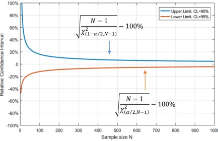
For a given sample size, the confidence bounds of uncertainties on core output re-sponses could be quantified using central limit theorem if normality assumption is valid. If a simple random sample sizeN is obtained from a normally distributed population with true meanµand true standard deviationσt r u e, then the following constructed parameter
χ2:
χ2=(N −1)σ 2 c a l c.
σ2 t r u e
(2.14)
follows a chi-square distribution with N - 1 degree of freedom, whereσ2
c a l c.is the sample variance. For a two-sided uncertain parameter, the criteria of 95% confidence level indicates that 95% of theχ2value is bounded inside the interval of[χ2
1−α/2,χ 2
interval of the standard deviationσt r u e could also be derived as Eq. 2.15: (N −1)σ2
c a l c.
σ2 α/2
≤σ2t r u e ≤
(N−1)σ2 c a l c.
σ2 1−α/2
(2.15)
In this study, the relative uncertainties, namely the ratio of the standard deviation to the mean value, are calculated for some of the important physics parameters. By increasing the sample size, the confidence intervals can be narrowed down, as illustrated in Figure 2.3
CHAPTER
3
INVESTIGATION OF CORRELATIONS
BETWEEN DIFFERENT PHYSICS
DOMAINS
core uncertainty quantifications are evaluated. Different correlations, including NK-FM, NK-TH, NK-FM-TH are considered and their impact on the estimation of uncertainties of core outputs are investigated.
3.1
Multi-physics Model of the PWR Mini-Core
The Organisation for Economic Co-operation and Development (OECD) Nuclear Energy Agency (NEA) has been developing an international benchmark of the light water reactor uncertainty analysis in modeling (LWR-UAM) to examine the uncertainty quantification and propagation methodologies with various simulation tools. The problem selected is a PWR mini-core problem based on the Three Mile Island unit 1 reactor. As shown in Figure 3.1, the PWR mini-core contains 9 fuel assemblies. Each assembly includes 208 fuel rods with a uranium enrichment of 4.12%, 16 guide tubes, and 1 instrumental tube in each assembly[17, 18].
Figure 3.1PWR mini-core radial layout.
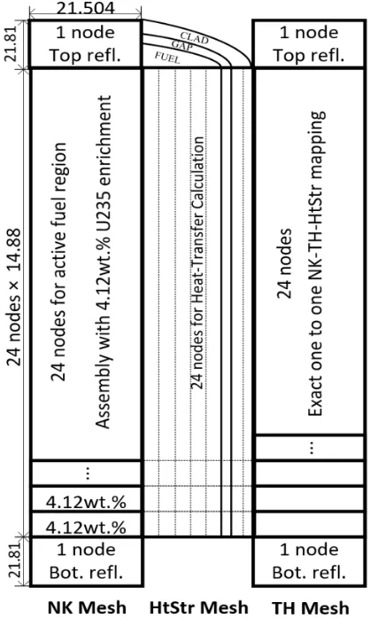
and no cross-flow between different PIPEs are considered. The fuel assembly is represented by its average fuel rod. Generally, each of the fuel assemblies is modelled using its own heat structure component (FM). As shown in Figure 3.3, the discretization decision allows an exact one-to-one mapping among TH, FM, and neutronic nodes, which provides exact feedbacks without homogenization during multi-physics core simulation.
Figure 3.2Conventional two-step LWR simulation approach.
Figure 3.3Heat conduction (HtStr) and thermal-hydraulics (TH) model, axial NK-FM-TH map-ping.
and control rod insertion fuel assembly and reflectors. The ranges of those state variables are determined such that both steady state and transient conditions at both BOC and EOC are covered. Depletion calculation was performed with 15 burnup points ranging from 0 to 40 GWD/MTU. Due to the limitation in Polaris modelling capability, the spacer grid cannot be explicitly modelled. Therefore, an additional cladding has been placed surrounding the fuel rod to account for the effect of spacer grid based on spacer grid mass conservation.
An example of the parametric structure of the cross section of fuel assemblies is depicted in Figure 3.4. Letρbe the moderator density,Tf the Doppler temperature,c the boron
concentration, and B u the burn-up, then the group homogenized macroscopic cross section in a specific state condition of(ρ,Tf,c,B u)could be calculated with reference value
Σr obtained at condition of(ρr,Tr f ,c
r,B ur)and the derivatives with respect to different
state variables as:
Σ(ρ,Tf,c,B u) =Σr+ ∂Σ
∂ ρ(ρ−ρ r) +1
2
∂Σ2
∂ ρ2(ρ−ρ
r)2+ ∂Σ
∂p
Tf (Æ
Tf − Æ
Tf r
)
+∂Σ
∂c (c −c
r) + ∂Σ
∂B u(B u−B u r)
(3.1)
3.2
Events Description
Numerical simulation at steady state and control rod ejection under hot full power condition is studied in this paper based on the PWR mini-core model specification. At hot full power, the nominal power of the core at hot full power is 140.9 MWt with inlet mass flow rate of 915 kg/s under system pressure of 15 MPa. Critical boron concentration search is performed to bring the reactor core into a critical state, at which the control rod ejection transient is initiated. The control rod located in the central assembly is withdrawn at a constant speed for 10 seconds until it reaches a distance corresponding to 20% of the active core height. The total simulation time of the transient process is set to be 600 seconds such that the reactor core reaches another stable state.
3.3
Verification of VCM Generation
The first step of this study is to verify that the use of the VCM carries the correct correlation information and propagates input uncertainty through the two-step core simulation cor-rectly. The following two cases are designed, and the uncertainty quantification results are compared to verify the effectiveness of the generated global VCM. Noted that at this step, only nuclear data uncertainty is considered, and the VCM only includes variables from the few-group constants.
• Case 1:n sets of few-group constants are generated using Polaris with uncertainty coming only from nuclear data uncertainty. The correspondingn core simulation runs are performed and the uncertainties of the output responses are calculated. Since this procedure involves the physical generation of the few-group constants, the uncertainties of output responses are used as references in the comparative analysis. • Case 2: A global VCM is estimated using the few-group constants generated in Case
global VCM. The correspondingn core simulation runs are executed, and the output responses are analyzed and compared with results obtained in Case 1.
Figure 3.5Correlation matrix of few-group constants.
shown in Figure 3.6.
Figure 3.6Correlation matrix for PWR mini-core problem.
concentra-tion, and two control rod states, at 3 burnup points (0, 15 and 30 MWD/T). Therefore, the generation of few-group constants in the lattice calculation is computationally expensive. In this study,n =500 sets of few-group constants are generated. Figure 3.5 depicts the correlation matrix obtained at one state data point.
The correlation coefficient, ranged from -1 to+1, is a measurement of the strength of the associations between the two variables. A large absolute magnitude of the correlation coefficient means the variation of one variable has a strong impact on the variation of the other variable. Positive correlation indicates that both variables increase or decrease together, whereas negative correlation indictes an decrease of one variable will increase the other, and vice versa. It is observed that the 6 group delayed neutron fractions and decay constants are strongly correlated between them but are not strongly correlated with the rest of the few-group constants. Radiative capture cross-section has a negative correlation with assemblyki n f, while the correlations betweenki n f and fission cross-section or the average
total number of neutron release per fission are positive. The capture cross-section and fission cross-section are both components of the total absorption cross-sections, and as a result, a negative correlation coefficient is observed in Figure 3.5. In the lattice calculation, the fuel assembly is symmetric and a reflective boundary condition is used. As a result, the assembly discontinuity factors (ADFs) are the same for the four faces, and corner discontinuity factors (CDFs) with symmetrical locations and directions are also identical. Therefore, only two ADFs from different energy groups and 4 CDFs are input variables to be included in the global VCM.
re-sampling data accurately recover the distribution of the original data.
Figure 3.7Distributions of original data (left), inverse transform sampling of CDF (mid.), and comparison of the distributions between original data and re-sampling data.
Both steady state simulation and control rod ejection transients are simulated under case 1 and case 2 configurations, where the original and re-sampling few-group constants are used, respectively. Figure 3.9 presents the comparison of the radial power distribution with associated relative standard deviations.
Figure 3.8 depicts the mean and associated uncertainties obtained with a different number of samples. It is found that the mean value and standard deviation converge after 100 samples, for both cases.
It can be observed that the mean value and uncertainty predicted with the few-group constants re-sampled using the global VCM agrees with those obtained using the origi-nal data quite well, despite that the re-sampling process tends to predict slightly larger uncertainty.
Figure 3.9Radial power distributions with associated uncertainties corresponding to case 1 (left) and case 2 (right).
Figure 3.10 presents the time evolutions of peak reactivity, power and fuel centreline temperatures. It can be observed that for both cases, the mean values of the output re-sponses agree perfectly with the nominal values. The trends of the time evolution of output responses agree with each other comparing the two cases. The 95% of the distribution of output responses are also plotted.
Figure 3.10Time evolution of core reactivity, total core power, and peak fuel temperatures under case 1 (left) and case 2 (right) configurations.
unknown and requires more investigation.
3.4
Correlation of Input Parameters
Input parameters are correlated due to the fact that their uncertainties may stem from the same source. For demonstration purposes, the uncertainties of the fuel rod radius (Rf u e l),
the gap size (e) between fuel rod and cladding inner surface, and cladding thickness (Tc l a d)
Table 3.1Summary of core output responses comparing case 1 and case 2.
Output Responses Case 1 Case 2
Steady state critical boron concentration 255±63 pcm 247±76 pcm Steady state axial power peakingFz 1.379±0.15% 1.385±0.19%
Steady state radial power peakingFR 1.242±0.27% 1.243±0.28%
Transient peak reactivity 0.55794+0.02023 ($) 0.55863+0.02095 ($)
Transient peak power 5.91+0.206 6.18+0.209
Transient peak fuel temperature 2367+127.6 (K) 2364+135.9 (K)
few-group constants are generated from lattice physics code Polaris as described in Section 3.1. The manufacturing uncertainties related to geometry are given in Table 3.2.
Table 3.2Summary of the geometrical manufacturing uncertainties considered for PWR mini-core problem.
Parameters Distribution Rel. Std.
Rf u e l Normal 0.99 %
Tc l a d Normal 0.89%
e Normal 5.25%
The thermal-hydraulic diameter (Dh), cross-sectional area (Ax) and wetted perimeter
(Pw) of the TH channel, and the gap conductance (Hg a p) are selected as representative TH
and FM variables.
Dh=
4Ax Pw
(3.2)
Ax=Pi t c h2 −πR 2
c l a d (3.4)
where, Dh is the thermal-hydraulics diameter, Ax is the cross-sectional area,Pw is the
wetting perimeter of the TH channel, respectively.Pi t c h is the pitch of the fuel assembly
andRc l a d is the cladding outer radius.
Hg a p= kg a s
e (3.5)
e=Rc l a d−Tc l a d−Rf u e l (3.6) Hg a p can be simply modeled as the ratio of the gas conductivitykg a s to pellet-cladding
gap widthe. The gap widthe can be further computed byRc l a d, cladding thicknessTc l a d
and fuel rod radiusRf u e l. The input parameters for core multi-physics simulation, namely
few-group neutronic constants, fuel modelling parameters and thermal-hydraulics param-eters are computed. The corresponding global variance-covariance matrix is constructed. Latin Hypercube Sampling is performed to generaten=500 sets of samples and the cor-responding core simulations are performed. Three different comparative studies are per-formed, with each study investigating the impact of correlations between different physics domains on core uncertainty quantification.
• Study 1: NK-TH correlations are considered. Uncertainties originating from geo-metrical manufacturing uncertainties are propagated into few-group constants and thermal-hydraulics parameters (Dh,Ax andPw) to estimate the corresponding VCM.
The VCM is re-sampled to propagate the uncertainty to steady state and rod ejection transient core simulations.
• Study 2: NK-FM correlations are considered with uncertainties originating from geometrical manufacturing uncertainties are propagated into NK few-group con-stants and FM parameters (Hg a p) to estimate the corresponding VCM. The VCM is
core simulations.
• Study 3: NK-TH-FM correlations are considered with uncertainties originating from geometrical manufacturing uncertainties.
3.4.1
NK-TH Correlation Study
The thermal-hydraulic model of the PWR generally requires the thermal-hydraulic diameter, cross-sectional area and volume of the TH channel as the inputs. In TRACE code, the PIPE channel represents ths average TH channel in the fuel assembly and the uncertainties of those three parameters are affected by the input uncertainties of fuel rod radius, gap thick-ness, and cladding thickthick-ness, as shown in Eq. 3.2 - 3.6. The global VCM can be constructed as shown in Figure 3.15. In order to quantify the impact of the correlations between NK and TH physics domains, the following two cases are designed:
• Correlated Case: The generated global VCM is sampledn times. The core simulations are performed with the sampled data and core output responses are analyzed. • Uncorrelated Case: The uncorrelated NK-TH VCM is obtained by removing the
co-variance terms between NK and TH parameters, as shown in the right figure of Figure 3.15. The altered global VCM is then sampled forntimes for realizations. Noted the generated realizations only reflect correlations in standalone NK or TH parameters, and the correlation between parameters of different physics domains has been re-moved. The corresponding core simulations are performed and output responses are analyzed. The sample size is 500 for both uncorrelated and correlated case.
Figure 3.11Time evolution of core reactivity, total core power, and peak fuel temperatures under case 1 (left) and case 2 (right) configurations.
Figure 3.12Running sample mean and uncertainty of the critical boron concentration at corre-lated case (left) and uncorrecorre-lated case (right).
Figure 3.13Radial power distributions with associated uncertainties corresponding at correlated case (left) and uncorrelated case (right).
Figure 3.14Time evolution of peak fuel temperatures under at correlated case (left) and uncorre-lated case (right) configurations.
3.4.2
NK-FM Correlation Study
Table 3.3Impact of the correlated and uncorrelated input uncertainties on core outputs by taking into account NK-TH correlations.
Output Responses Correlated case Uncorrelated case
Steady state critical boron concentration 256±29 (pcm) 255±31 (pcm) Steady state axial power peakingFz 1.379±0.05% 1.379±0.05%
Steady state radial power peakingFR 1.242±0.02% 1.242±0.07%
Transient peak reactivity 0.55736+0.00323 ($) 0.55734+0.00464 ($)
Transient peak power 5.91+0.08473 5.92+0.11102
Figure 3.15Correlation between few-group constants and gap conductance (NK-FM correlation).
Table 3.4 presents the impact of NK-FM correlation on core uncertainty analysis. It is observed that by taken into account the NK-FM correlations, the corresponding core responses is predicted with smaller uncertainties. For example, the uncertainty of peak fuel temperature is decreased by 9 K.
Table 3.4Impact of the correlated and uncorrelated input uncertainties on core outputs by taken into account NK-FM correlations.
Output Responses Correlated case Uncorrelated case
Steady state critical boron concentration 260±35 (pcm) 256±36 (pcm) Steady state axial power peakingFz 1.387±0.06% 1.391±0.06%
Steady state radial power peakingFR 1.245±0.08% 1.253±0.09%
Transient peak reactivity 0.55699+0.00353 ($) 0.55634+0.00465 ($)
Transient peak power 5.95+0.08994 5.96+0.11473
Transient peak fuel temperature 2390+33 (K) 2381+42 (K)
3.4.3
NK-FM-TH Correlation Study
In this study, the correlations between few group constants, gap conductance and thermal-hydraulics modelling input parameters (Dh,Ax, andPw) are considered. The correlated case
Table 3.5Impact of the correlated and uncorrelated input uncertainties on core outputs by taken into account NK-TH correlations.
Output Responses Correlated case Uncorrelated case
Steady state critical boron concentration 259±40 pcm 250±48 pcm Steady state axial power peakingFz 1.371±0.20% 1.379±0.22%
Steady state radial power peakingFR 1.232±0.30% 1.242±0.32%
Transient peak reactivity 0.55864+0.02304 ($) 0.55833+0.02415 ($)
Transient peak power 6.09+0.2175 6.15+0.2381
Transient peak fuel temperature 2367+56.8 (K) 2374+69.5 (K)
3.5
Summary
CHAPTER
4
CONSISTENT UNCERTAINTY ANALYSIS
OF THE TMI-1 REACTOR CORE
4.1
TMI-1 Reactor Core
The TMI-1 nuclear power plant is a PWR designed by Babcock & Wilcox with a rated power of 2772M Wt h. The power plant has a wet-recirculating system for cooling using two
nat-ural draft cooling towers. The reactor core consists of 177 fuel assemblies, and each fuel assembly has 208 fuel rods, 16 guide tubes, and 1 tube for the instrumentation. There are 11 types of fuel assemblies in the TMI-1 active core with various fuel enrichment (4.00%, 4.40%, 4.85%, 4.95%, and 5.00%) and configurations with regard to the configuration of the burnable poison (BP), gadolinia pins (GdO2+UO2) and control rod banks. The quarter core representation is depicted in Figure 4.1 where assembly H8 is located in the core center. Detailed geometry setup and fuel modelling parameters can be found in the benchmark specification[12].
4.2
Numerical Test Cases
Numerical test cases BOC and EOC steady state and control rod ejection under hot full power (HFP) condition were studied in this paper based on TMI-1 operational data for initial conditions. For steady-state calculations, boron concentration is set to be 1935 ppm and 5 ppm at BOC and EOC, respectively. At hot full power condition (HFP), control rod bank 1-6 (Figure 4.1) are completely withdrawn, bank 7 is completely inserted while the partial-length axial power shape rod (APSR) is 54% inserted. The rated power of the core at HFP is set to be 2772 MW with an inlet moderator temperature of 563 K. The mass flow rate is set to be 1.65 × 10⁴ kg/s under a system pressure of 15 MPa, and coolant flowing into different TH channels are pre-calculated and used as fixed boundary conditions in this study[12].
Figure 4.1TMI-1 quarter core configuration.
investigated to assess the core transient behavior.
The last case investigated in this study is the core cycle depletion calculation from BOC state to EOC state, as has been defined in the LWR-UAM Exercise 1 of Phase III. Reactor core is depleted at hot full power of 2771.9 MWth, with a nominal system pressure of 15.36 MPa. The mass flow rate through reactor core is assumed to be 16546.04 kg/s with inlet coolant temperature of 562.67 K. The estimated average fuel temperature and outlet coolant temperature is 921 K and 592.7 K, respectively. Control rod groups 1-6 are completed withdrawn, while group 7 and the axial power shape rod (APSR) is 90% and 30% withdrawn, respectively. The core is depleted for 664 EFPD with an estimated core average exposure of 42.06 GWD/MTU at EOC. The estimated critical boron concentration at EOC is 5 ppm.
4.3
Multi-Physics PWR Core Model
A reference TRACE/PARCS[28]model needs to be developed with a list of input uncertain parameters with associated distribution. This sub-section describes the specific neutronic-kinetic (NK) model, thermal-hydraulic (TH) model, as well as the coupling between the two. Generally, in order to perform a meaningful uncertainty propagation and quantification, the coupling scheme and reference model must be validated to be accurate enough. In the current stage, two coupling schemes were investigated, and the simulation results were compared in next Section to identify the impact of different coupling schemes on uncertainty quantification.
end of cycle (EOC) based on the reactor operational data. The average core exposure is 18 and 40 GWD/MTU at BOC and EOC, respectively.
Figure 4.2One Dimensional Channel model: TRACE TH, HTSTR models, and TH-HTSTR-NK mapping.
4.4
Uncertainty Analysis of PWR Steady State Simulation
Coreke f f and power peaking factors were selected as output responses of interest and
results at nominal state were summarized in 4.1. It is worth mentioning that no boron concentration adjustment was performed for steady state calculations, and theke f f at BOC
is slightly higher than expected, partially because the core was modelled with only 18 TH channels, which tends to predict a smaller control rod worth compared to the detailed one TH channel to one fuel assembly model, as revealed by[29]. The core simulation at EOC was performed with equilibrium concentration calculation of Xenon and Samarium, which were efficient neutron absorbers and brought the core to be 1.71 %∆k/k subcritical.
Table 4.1Core Physics Parameters at Nominal State.
Nominalke f f NominalFZ NominalFR NominalFq
BOC 1.01501 1.01501 1.349 1.776
EOC 0.98290 1.190 1.402 1.674
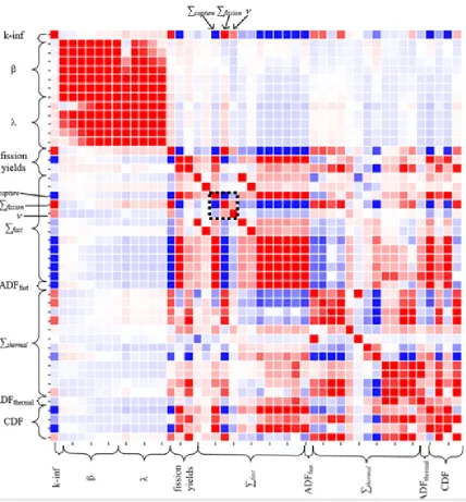
Figure 4.3Correlation matrix of few-group constants,Hg a p,Dh,Ax andPw.
and passed into Polaris for lattice calculation. As a result, 100 sets of input parameters (few-group constants,Hg a p,Dh,Ax andPw) are obtained. The corresponding global VCM
is computed as Eq. 2.3, as shown in Figure 4.3. By sampling the global VCM as described in Chapter 2 and 500 re-sampled input parameters are obtained, which are further passed into core multi-physics simulation using TRACE/PARCS as described in Chapter 4.3.
Table 4.2Summary of the geometrical manufacturing uncertainties considered for TMI-1 large-scale core problem.
Parameters Distribution Rel. Std.
Rf u e l Normal 0.99 %
Tc l a d Normal 0.89%
e Normal 5.25%
Nuclear Data ENDF/B-VII.1, SCALE 56-group VCM
400 samples and the standard deviation has also been stabilized.N =500 burnup dependent sets of perturbed input parameters were generated for each of the assembly types. It should be noted that for the multi-physics thermal-hydraulics model, several fuel assemblies are represented with one TH channel. Therefore, the thermal-hydraulics parameters, namely theDh,Ax,Pw, are computed for the average fuel rod of the TH channel. Uncertain fuel
modelling parameters considered in this study were gap conductance with uncertainties from geometrical manufacturing uncertainties. The correlations between different physics domain are considered Following the Eq. 2.15, the true standard deviationσt r u e of a two-sided distribution are bounded by[94%σc a l c., 106%σc a l c.]with 95 % confidence level, whereσc a l c.is the standard deviation calculated from 500 samples. The uncertainty of
σt r u e could be reduced by increasing sample size (narrows down to[96%σc a l c., 105 %
σc a l c.]for sample size of 1000). It should be noted that the calculated confidence intervals are only valid given that the output response of interest is normally distributed.
Table 4.3 presents the overall results of coreke f f, axial power peaking factors (FZ), and
radial power peaking factors (FR) for two core states given in the form of sample mean
and relative standard deviation. A relatively small uncertainty ( 0.5 %) was found for most cases, while the uncertainties forFZ at EOC and FR were relatively larger (>0.6 %), basically
Figure 4.4Running meanke f f for HFP at BOC.
Figure 4.5Running meanke f f for HFP at EOC.
at the 5t h for the rest.
Table 4.3Summary of the geometrical manufacturing uncertainties considered for TMI-1 Reactor Core Steady State Simulation.
State Statistics ke f f Fz FR
BOC Mean±rel.σc a l c. 1.01501±0.51% 1.32±0.52% 1.35±0.62%
σt r u e [0.45%, 0.54%] [0.49%, 0.55%] [0.58%, 0.66%]
AD normality test Pass Pass
EOC Mean±rel.σc a l c. 0.98295±0.45% 1.19±0.63% 1.40±0.82%
σt r u e [0.42%, 0.48%] [0.59%, 0.67%] [0.77%, 0.87%]
AD normality test Pass Pass Pass
normality tests are also performed for the keff and power peaking factors. The calculated A2 for core responses are less than 0.757, as shown in Table 4.3. It could be interpreted as that the distance from ECDF of the sample distribution to the CDF of the re-constructed perfect normal distribution is less than the critical threshold (0.757) and the probability of observing an equal or even smaller distance is greater than the pre-determined significant level of 0.05. It could be concluded that the sample populations of all the four core responses are significantly drawn from normal distributions, which could be fully described by providing the means and standard deviations.
Figure 4.6Frequency histogram of core key axial power peaking factors at HFP EOC state.
corresponds to different assembly compositions and material properties.
Table 4.4A2and correspondingp−v a l u e s for power peaking factors at various core states.
State Fz (M1) Fz (M2) FR (M1) FR (M2)
BOCA2 0.251 0.265 0.236 0.322
EOCA2 0.365 0.463 0.536 0.368
BOCp−v a l u e s 0.212 0.439 0.155 0.356
EOCp−v a l u e s 0.433 0.531 0.326 0.461
Figure 4.7Core axial power under HFP BOC and HFP EOC steady states.
Figure 4.8Radial power distribution at BOC .
larger uncertainty was observed at BOC compared to EOC, as fuel assemblies are higher enriched at BOC condition.
Figure 4.9Radial power distribution at EOC.
have the largest contribution to all three core output responses. FM (Hg a p) and TH related
parameters have only small impact (<0.11%) on core steady stateke f f and power peaking
factors.
4.5
Uncertainty Analysis of PWR Transient Simulation
Table 4.5Summary of uncertainty quantification on selected core parameters at steady state simulations (numbers given in mean±relative standard deviation).
Source of uncertainty State Sampleke f f SampleFZ SampleFR
Correlated BOC 1.01501±0.51% 1.32±0.52% 1.35±0.62%
EOC 0.98295±0.45% 1.19±0.63% 1.40±0.82% Uncorrelated BOC 1.01511±0.53% 1.32±0.52% 1.35±0.64% EOC 0.98290±0.46% 1.19±0.64% 1.40±0.86% NK few-group constants only BOC 1.01503±0.50% 1.32±0.50% 1.34±0.53% EOC 0.98294±0.43% 1.19±0.53% 1.41±0.51%
FM only BOC 1.01511±0.03% 1.31±0.11% 1.35±0.09%
EOC 0.98284±0.01% 1.19±0.09% 1.40±0.08%
TH only BOC 1.01496±0.03% 1.32±0.06% 1.35±0.02%
EOC 0.98290±0.04% 1.19±0.05% 1.40±0.03%
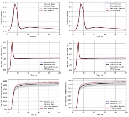
reactivity insertion and smaller gap conductance at BOC. It is worth mentioning that in this study the peak fuel temperature is defined as the maximum temperature of fuel that can be found in any location of the core and thus is a location-free value. Consequently, when the peak location of the fuel temperature changes during the transient, it can cause “disconti-nuity” in the time evolution curve of the fuel temperature. For example, the “jump” that occurred at 5-10 s for almost all cases at EOC is caused by the shift of the fuel temperature peak location from L11 to M12.
Figure 4.10Core net reactivity during transient, initiated from HFP at BOC.
Figure 4.11Core net reactivity during transient, initiated from HFP at EOC.
Figure 4.12Normalized core power during transient, initiated from critical HFP at BOC.
Figure 4.13Normalized core power during transient, initiated from critical HFP at EOC.
Figure 4.14Peak fuel temperature during transient, initiated from HFP at BOC.
TH (hd,Pw andV o l) related parameters also have non-negligible contributions. It is also
observed thatHg a p shows larger impact on peak fuel temperature at BOC than EOC, which
Figure 4.15Peak fuel temperature during transient, initiated from HFP at EOC.
Table 4.6Summary of uncertainty quantification for TMI-1 REA transient simulations (numbers given in mean+ [95t h/95% tolerance limit - mean]).
State Peak Core
Reactivity ($)
Peak Core Total Power
Peak Fuel
Temperature (K) Correlated BOC 0.405421+0.07253 1.71+16.3% 2598+106
Correlated EOC 0.418030+0.10068 1.65+24.3% 1810+89 Uncorrelated BOC 0.405389+0.07356 1.69+17.1% 2593+148 Uncorrelated EOC 0. 418145+0.10165 1.63+25.5% 1815+95
4.6
Uncertainty Analysis of PWR Cycle Depletion Simulation
Figure 4.16 presents the core burnup distribution predicted by PARCS/PATHS[30]in the unperturbed case. The reference solutions of assembly burnups can be found in LWR-UAM benchmark specification, and the maximum relative error of the simulation results is found to be -1.39%. The calculated critical boron concentration at EOC is 38 ppm, which compares favorably with the reference solution with an error of 33 ppm.
Figure 4.16Core Burnup Distribution and Relative Error at EOC.
uncertainties.
Figure 4.17Burnups at EOC with Associated Uncertainties with consideration of NK-FM-TH correlations.
4.7
Summary
This Chapter demonstrates the uncertainty analysis of the TMI-1 core multi-physics simula-tions, including steady state simulation, control rod ejection transient and cycle depletion calculations. The input uncertainties considered includes nuclear data uncertainties and geometrical manufacturing uncertainties, whose uncertainties are propagated into few-group constants (NK), gap conductance (FM) and parameters related to thermal-hydraulics modelling (TH). A global VCM can be generated to represent the correlation between dif-ferent physics domains. The final core output responses are calculated with associated uncertainties. By taking into consideration of the NK-FM-TH correlations, the uncertainties of core output responses are reduced. For example, the prediction of the 95% peak fuel temperature at BOC during control rod ejection accident is reduced by 37 K by considering the correlations.
CHAPTER
5
CONCLUSIONS AND FUTURE WORK
5.1
Conclusions
In this work, an innovative method for consistently propagating and quantifying uncertain-ties for the multi-physics PWR core simulation is developed based on stochastic sampling approach and demonstrated on the PWR benchmark problems.
The framework is firstly demonstrated in the PWR mini-core problem. The geometrical manufacturing uncertainties are considered and propagated into few-group constants, gap conductance and parameters related to TH model. By taking into account different correlations into account when sampling step of the global VCM, the impact of NK-FM, NK-TH, and NK-FM-TH correlations on core multi-physics steady state and transient simulations are studied. It is observed that the uncertainties of core outputs tends to be smaller when correlations are taken into account. For example, the uncertainty of peak fuel temperature at BOC during control rod ejection accident is 37 K smaller at BOC with the consideration of correlations than otherwise.
This consistent uncertainty analysis framework is further implemented in the uncer-tainty analysis of the TMI-1 core simulation. In the steady state calculations, the unceruncer-tainty for the coreke f f is found to be less than 0.6% and mainly contributed by the nuclear data.
The normality test suggests that the core ke f f and power peaking factors can both be
described by a normal distribution. The confidence intervals of core outputs are also com-puted and summarized. Time evolution of core reactivity, power, and peak fuel temperature as a result of an ejected control rod are also studied. Moreover, cycle depletion analysis is also performed and the uncertainties of assembly burnup is calculated. It is observed that the uncertainties of core output responses are decreased with consideration of the multi-physics correlations, which indicates that the safety margin is increased with consideration of the correlations.
5.2
Future Work
Although the main findings of this work is favourable, there are multiple aspects that can be done to improve the quality of this work. The major limitation of this work stems from the fact that only the geometrical manufacturing uncertainties and nuclear data uncertainties are considered, while there are many other important sources of input uncertainties were left out. For example, uncertainties related to fuel composition and fuel density during fuel rod fabrication are also important, and are expected to have impact on both fuel conductivity (for FM) and few group constants (for NK) simulation. In the future, a more detailed modeling using fuel rod modeling code (e.g. FRAPCON/FRAPTRAN) is recom-mended to evaluate the impact of fuel manufacturing uncertainties on fuel properties. The correlations between few-group constants and fuel properties due to fuel density and compositions uncertainties will need to be evaluated, and consistently propagated through core multi-physics simulation.
The work can also be improved by performing a more efficient sampling of the VCM. As demonstrated in Figure 3.6, the dimension of global VCM is large due to the fact that the few-group constants are generated at different data points of fuel temperature, moderator density, boron concentration, control rod insertion status and burnups. For large PWR core such as TMI-1 reactor core, this global VCM is even larger because there are 11 different types of fuel assemblies. The few-group constants related to different types of assemblies also needs to be considered, which further expands the size of VCM by 11 times. However, the few-group constants are highly linear between each other, which provides the potential possibility of reducing the size of the global VCM while maintaining the accurate represen-tation of the correlations. The principle component analysis (PCA) of the global VCM is suggested in the future to reduce the dimension of the matrix.
BIBLIOGRAPHY
[1] U.S.NRC. 10 CFR Part 50 - Definitions.URL:
https://www.nrc.gov/reading-rm/doc-collections/cfr/part050/part050-0002.html
.[2] Boyack, B. et al. “Quantifying Reactor Safety Margins Part 1: An Overview of the Code Scaling, Applicability, and Uncertainty Evaluation Methodology”.Nuclear
Engineer-ing and Design119(1990), pp. 1–15.
[3] Wilson, G. et al. “Quantifying Reactor Safety Margins Part 2: Characterization of Important Contributors to Uncertainty”.Nuclear Engineering and Design119(1990), pp. 17–31.
[4] Wulff, W. et al. “Quantifying Reactor Safety Margins Part 3: Assessment and Ranging of Parameters”.Nuclear Engineering and Design119(1990), pp. 33–65.
[5] Lellouche, G. et al. “Quantifying Reactor Safety Margins Part 4: Uncertainty Evaluation of LBLOCA Analysis Based on Trac-PF1/Mod 1”.Nuclear Engineering and Design 119(1990), pp. 67–95.
[6] Zuber, N. et al. “Quantifying Reactor Safety Margins Part 5: Evaluation of Scale-Up Capabilities of Best Estimate Codes”.Nuclear Engineering and Design119(1990), pp. 97–107.
[7] Catton, I. et al. “Quantifying Reactor Safety Margins Part 6: A Physically Based Method of Estimating PWR Large Break Loss of Coolant Accident PCT”.Nuclear Engineering
and Design119(1990), pp. 109–117.
[8] Glaeser, H. “Evaluation of Licensing Margins of Operating Reactors Using ‘Best Esti-mate Methods Including Uncertainty Analysis”.5th Seminar on Scaling Uncertainty
and 3D Coupled Code Calculations in Nuclear Technology(2006).
[9] Rohatgi.Historical perspectives of BEPU research in United States. Brookhaven Na-tional Laboratory, 2018.
[10] Ivanov, K. et al. “Uncertainty Analysis in Reactor Physics Modeling”.Science and
Technology of Nuclear Installations2013(2013), pp. 1–2.
[11] Ivanov, K. et al.Benchmarks for Uncertainty Analysis in Modelling (UAM) for the Design, Operation and Safety Analysis of LWRs. Volume I: Specification and Support
Data for Neutronics Cases (Phase I). OECD NEA, 2013.
[12] Hou, J. et al.Benchmarks for Uncertainty Analysis in Modelling (UAM) for the Design, Operation and Safety Analysis of LWRs. Volume III: Specification and Support Data
[13] Wieselquist, W. et al. “PSI Methodologies for Nuclear Data Uncertainty Propagation with CASMO-5M and MCNPX: Results for OECD/NEA UAM Benchmark Phase I”.
Nuclear Engineering and Design2013(2013), pp. 1–15.
[14] Zeng, K. et al. “Uncertainty Analysis of Light Water Reactor Core Simulations Using Statistic Sampling Method”.MC 2017(2017).
[15] Hou, J. et al. “Comparative Analysis of Solutions of Neutronics Exercises of the LWR UAM Benchmark”.MC 2019(2019).
[16] Porter, N. et al. “Uncertainty Quantification Study of CTF for the OECD/NEA LWR Uncertainty Analysis in Modeling Benchmark”.Nuclear Science and Engineering 192(2018), pp. 271–286.
[17] Radaideh, M. et al. “Sampling-based Uncertainty Quantification of the Six-group Kinetic Parameters”.Reactor Physics Paving the Way Towards More Efficient Systems
(2018).
[18] Zeng, K. et al. “Uncertainty Quantification and Propagation of Multiphysics Simula-tion of the Pressurized Water Reactor Core”.Nuclear Technology205(2019), pp. 1618– 1637.
[19] Delipei, G. “Multi-Physics Uncertainty Propagation in a PWR Rod Ejection Accident Modeling - Analysis Methodology and First Results”.BEPU2018(2018).
[20] Zeng, K. et al. “Impact of Spatial Coupling Schemes and Perturbation Options on Uncertainty Quantification of PWR Core Simulation”.MC 2019(2019).
[21] Yankow, A. “A Two-Step Approach to Uncertainty Quantification of Core Simulators”.
Science and Technology of Nuclear Installations2012(1954), pp. 765–769.
[22] Anderson, T. “A Test of Goodness of Fit”.Journal of the American Statistical Associa-tion49(2012), pp. 1–9.
[23] Henderson, K. “Testing Experimental Data for Univariate Normality”.Clinica Chimica Acta366(2006), pp. 112–129.
[24] Downar, T. et al.PARCS v3.0 U.S. NRC Core Neutronics Simulator User Manual. Uni-versity of Michigan, 2012.
[25] Bajorek, S. et al.TRACE V5.0 Patch 5 User’s Manual. U. S. Nuclear Regulatory Com-mission, 2016.
![Figure 1.1 Concept of BEPU approach and the benefit of BEPU analysis compared to conserva-tive analysis [9].](https://thumb-us.123doks.com/thumbv2/123dok_us/1769116.1227667/15.612.92.536.77.394/figure-concept-approach-benet-analysis-compared-conserva-analysis.webp)