An optimal method for approximating the delay differential equations of noninteger order

R E S E A R C H

Open Access

An optimal method for approximating the

delay differential equations of noninteger

order

Dumitru Baleanu

_{, Bahram Agheli}

_{and Rahmat Darzi}

*_{Correspondence:} [email protected] 1_{Department of Mathematics,} Çankaya University, Ankara, Turkey 2_{Institute of Space Sciences,} Maturely-Bucharest, Romania Full list of author information is available at the end of the article

Abstract

The main purpose of this paper is to use a method with a free parameter, named the optimal asymptotic homotopy method (OHAM), in order to obtain the solution of delay differential equations, delay partial differential equations, and a system of coupled delay equations featuring fractional derivative. This method is preferable to others since it has faster convergence toward homotopy perturbation method, and the convergence rate can be set as a controlled area. Various examples are given to better understand the use of this method. The approximate solutions are compared with exact solutions as well.

MSC: 35R11; 65F10; 26A33

Keywords: Delay differential equations; Optimal homotopy asymptotic; Caputo derivative

1 Introduction

Fractional arithmetic and fractional differential equations appeared in many disciplines, including medicine [1], economics [2], dynamical problems [3,4], chemistry [5], mathe-matical physics [6], traffic model [7], fluid flow [8], and so on.

Scholars and researchers are invited to study books that have been written to better un-derstand the concept of fractional arithmetic [9–11]. The fractional differential equations with delay inxare not very well realized. To find the approximate solution for delay dif-ferential equations with fractional derivative that we explore in this paper is presented as follows:

Dα_xu(x) +Ax,u(p0x),ux(p1x),uxx(p3x), . . . ,ux · · ·x

norder

(pnx)

=g(x) (1.1)

with the initial conditions

ux(0) =μ0, . . . , ux · · ·x

norder

(0) =μn,

where μn is a constant,g(x) is a known analytic function, 0≤x≤1, pj∈R for j=

0, 1, 2, . . . ,n,Ais the differential operator, andDα

tive of orderαgiven by

Dα

xu(x) =

1

(k+ 1 –α)

x

0

(x–s)k–α_u(k+1)_{(s)ds, k<α≤k+ 1,k∈Z}+_{. (1.2)}

These equations for α= 1 appear in the mathematical and physical modeling of time-dependent process, and their goal is to determine the rate of change of the current situa-tion in comparison with the former models. In particular, this conversion is basic when an ordinary differential equation is based on model failure. Among these types, there are pan-tograph differential equations , which have been of interest to many researchers. A panto-graph is a machine that rolls up an electric current from upper lines for trams or electric trains. The term pantograph has been retrieved from its similarity to pantograph machines for drawings copying and writing [12–14]. About the existence of solutions for these equa-tions, we can mention [15,16].

The fractional differential equations with shrinking in xand delays int are not very well realized. So we look for an approximate solution for delay differential equations with fractional derivative of the following form:

Dα

tu(x,t) +A

x,t,u(p0x,q0t),ux(p1x,q1t),uxx(p3x,q3t), . . . ,ux · · ·x

norder

(pnx,qnt)

=g(x,t) (1.3)

with the initial conditions

ut(x, 0) =h0(x), . . . ,ut · · ·t norder

(x, 0) =hn(x),

whereg(x,t) is a known analytic function,t> 0, 0≤x≤1,pj,qj∈Rforj= 0, 1, 2, . . . ,n, Ais the partial differential operator, andDα

t denotes the fractional Caputo derivative of

orderαgiven by

Dα_tu(x,t) = 1

(k+ 1 –α)

t

0

(t–s)k–α

u(k+1)(x,s)ds, k<α≤k+ 1,k∈Z+. (1.4)

The delay differential equations (DDEs) and fractional delay differential equations (FDDEs) appear in modeling different problems in engineering and science such as bi-ology models [17,18], control theory [19,20], oscillation theory [21,22], delay systems [23,24], and so on.

A number of papers that can be found in modeling, deploying and extending delay dif-ferential equations, delay partial differential equations, and fractional delay differential equations [25,26].

31], Adomian’s decomposition method (ADM) [31], the optimal homotopy asymptotic method (OHAM) [32], the homotopy analysis method (HAM) [33–35], the variational iteration method (VIM) [36], and so on [37–40].

This paper is organized as follows. In Sect.2, we give a description of OHAM. In Sect.3, we express the convergence of OHAM. In Sect.4, applications of OHAM to Eqs. (1.1) and (1.3) are illustrated, and some numerical examples are presented. Conclusions are drawn in Sect.5.

2 Description of OHAM

The overall dimensions of the proposed approach [41] in this section are given and repre-sented in the following differential equation:

Lu(x,t)+Nu(x,t),uη0(x),ς0(t)

,ux

η1(x),ς1(t)

, . . . ,ux · · ·x norder

ηn(x),ςn(t)

+g(x,t) = 0, x∈⊆Rn,t> 0, (2.1)

with boundary condition

B u,∂u

∂t

= 0, t∈, (2.2)

whereL=Dα

t is a linear operator,Nis a nonlinear operator consisting of the space

deriva-tives of integer order with respect toxalong with delay functions,u(x,t) is an unknown function,g(x,t) is a known analytic function,Bis a boundary operator, andis the bound-ary of the domain; also,ηj(x) andςj(t) are delay functions. In this work, we consider ηj(x) =pjxandςj(t) =qjtforj= 0, 1, . . . ,n.

According toOHAM, we concoct structural homotopyv(x,t;p) :×[0, 1]→Rthat fulfills the conditions in the following equation:

(1 –p)Lv(x,t;p) –u0(x,t)

=H(p)(Lv(x,t;p)+g(x,t) +Nu(x,t),uη0(x),ς0(t)

,ux

η1(x),ς1(t)

, . . . ,ux . . .x norder

ηn(x),ςn(t)

, (2.3)

where p∈[0, 1] is an infix parameter. The supporting function H(p) is elected in the following display as a nonzero forp= 0 andH(0) = 0. Whenp= 0 andp= 1, we have

v(x,t; 0) =u0(x,t) andv(x,t; 1) =u(x,t).

Thus, whenpvaries from 0 to 1, the solutionv(x,t;p) approaches from the initial guess

u0(x,t) to exact solutionu(x,t);u0(x,t) obtained from (2.2) to (2.3) withp= 0 giving

Lu0(x,t; 0)

+g(x,t) = 0. (2.4)

The functionH(p) is assumed to be

in whichc1,c2,c3, . . . are the convergence control parameters, which are unfamiliar and

can be calculated. Another demonstration formH(p) is offered by Herisanu and Marinca [41].

We consider the zero-order problem (2.4), the first-order equation

Lu1(x,t)

about the infix parameterp, and we have

The following residual is the result obtained as a result of embedding (2.12) in (2.1):

R(x,t;ci) =L

˜

v(x,t;p,ci)

+g(x,t) +Nv˜(x,t;p,ci)

, i= 1, 2, . . . ,m. (2.13)

IfR= 0, thenv˜is the exact solution of (2.1).

Using the method of least squares and knowing the exact solution of the problem, we can minimize theL2_{-norm of the errorEv}

m(c1,c2,c3, . . . ,cm). TheL2-norm of the error is _{Evm(c1, . . . ,cm)}

2=

v2_m(x,t)dt dx

1 2

,

whereEvm(x,t) =|vexact(x,t) –vm(x,t;c1, . . . ,cm)|. 3 Convergence of OHAM

In this section, we consider the convergence of theOHAM.

Theorem 3.1 ([42]) Let the solution components u0,u1,u2, . . . , be defined as given in

Eqs. (2.8)–(2.10).The series solutionm–1_k=0 uk(x,t)defined in(2.12)converges if there exists

0 <ρ< 1such that uk+1 ≤ρ uk for all k≥k0for some k0∈N.

Proof Consider the sequence{Tn}∞n=0defined as

T0=u0,

T1=u0+u1,

T2=u0+u1+u2,

. . . ,

Tn=u0+u1+u2+· · ·+un.

Evidently, it is sufficient to show that the sequence {Tn}∞n=0 in the Hilbert space Ris a

Cauchy sequence. To this end, consider

Tn+1–Tn = un+1

≤ρ un

≤ρ2 un–1

.. .

≤ρn–k0+1 _u k0 .

Assuming thatn≥m>k0,n,m∈N, we have

Tn–Tm =(Tn–Tn–1) + (Tn–1–Tn–2) +· · ·+ (Tm–Tm–1)

≤ρn–k0 _u

{Tn}∞n=0is a Cauchy sequence, and this implies that series solution converges to the series

∞

k=0uk(x,t).

4 Test examples

To understand OHAM, in this section, we describe and then calculate some examples. These examples include delay differential equations, delay partial differential equations, and a system of coupled fractional delay equations with fractional derivative. In all these examples, we used the mathematical softwareMathematicafor calculations and graphs.

Test example4.1 For the first example, we propose the FDDEs [43]

Dα_xu(x) + 2u x

Following theOHAM, according to what was formulated and presented in Sect.2for Eqs. (4.1)–(4.2), we get:

Then, considering the first three terms as estimates of solution for Eq. (4.1), we have

Table 1 Exact and approximate result of Test example4.1with various values ofα

x OHAM Exact Absolute error

α= 0.6 α= 0.8 α= 1

0.0 0.0 0.0 0.0 0.0 0.0

0.2 0.380402 0.283984 0.193419 0.198669 0.00525038 0.4 0.423057 0.475332 0.383577 0.389418 0.00584113 0.6 0.17166 0.598362 0.564596 0.564642 0.00004673 0.8 –0.472504 0.616461 0.725359 0.717356 0.00800265 1.0 –1.6197 0.471231 0.846895 0.841471 0.00542437

– 2c

2 1xα (α+ 1)+

25–4α_c3

1(4α)(α+12)x 5α

15√π α3_(α)2_(3α)(5α)+

2c3₁(α+1₂)x3α

√

π (α+ 1)(3α+ 1) + 2c2(α+

1 2)x3

α

√

π (α+ 1)(3α+ 1). (4.3) According to least square method for the calculations of the constantsc1 andc2, we get

c1= –2.01508,c2= 7.91742, which are called convergent control parameters.

In Table1, we can see the estimated solutions towardα= 1, which are derived for various values ofxapplyingOHAM. TheL2_{-norm of the error for Test example4.1ofα= 1 is}

0.00560315.

Test example4.2 For the second example, we consider the FDDEs

Dα

xu(x) – 2u

x

2

+u(x) = –x2– 1, 0≤x≤1, 2 <α≤3, (4.4)

with initial conditions

u(0) = 1, u(0) = –4, u(0) = 0. (4.5)

With the help of theOHAM, according to what was formulated and presented in Sect.2

for Eqs. (4.4)–(4.5), we get:

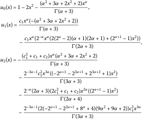
u0(x) = 1 – 2x2–

(α2+ 3α+ 2x2_{+ 2)x}α

(α+ 3) ,

u1(x) =

c1xα(–(α2+ 3α+ 2x2+ 2)) (α+ 3)

–c1x

α₍₂–α_xα₍₂₍₂α_{– 2)(α+ 1)(2α+ 1) + (2}α+1_{– 1)x}2₎₎

(2α+ 3) ,

u2(x) = –

(c21+c1+c2)xα(α2+ 3α+ 2x2+ 2) (α+ 3)

–2

–3α–1_c2

1x3α((–2α+1– 22α+1+ 23α+2+ 1)x2) (3α+ 3)

–2

–α_{(2α+ 3)(2c}2

1+c1+c2)x2α((2α+1– 1)x2) (2α+ 4)

–2

Table 2 Exact and approximate result of Test example4.2with various values ofα

x OHAM Exact Absolute error

α= 2.6 α= 2.8 α= 3

0.0 1.0 1.0 1.0 1.0 0.0

0.2 0.919879 0.91993 0.91996 0.92 0.00003957

0.4 0.679283 0.679518 0.679683 0.68 0.00031677 0.6 0.278073 0.278548 0.278943 0.28 0.00105659 0.8 –0.283555 –0.28302 –0.282416 –0.28 0.00241631 1.0 –1.00486 –1.00489 –1.00437 –1.0 0.00437343

–2

–α_{(2α+ 3)(2(2}α_{– 2)(2α}2_{+ 3α+ 1))(2c}2

1+c1+c2)x2α

(2α+ 4) ,

. . . .

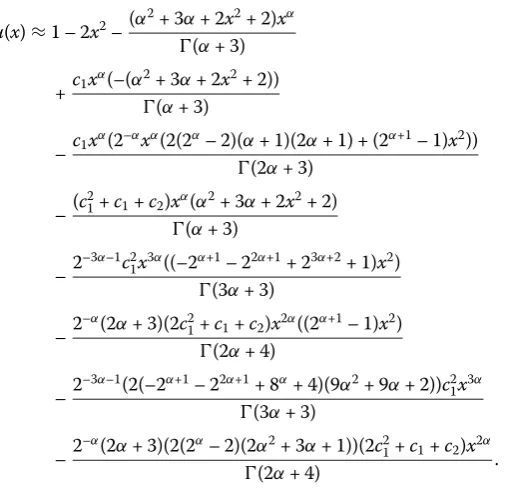
Then, considering the first three terms as estimates of solution for Eq. (4.4), we have

u(x)≈1 – 2x2–(α

2_{+ 3α+ 2x}2_{+ 2)x}α

(α+ 3) +c1x

α_(–(α2_{+ 3α+ 2x}2_{+ 2))} (α+ 3)

–c1x

α₍₂–α_xα₍₂₍₂α_{– 2)(α+ 1)(2α+ 1) + (2}α+1_{– 1)x}2₎₎ (2α+ 3)

–(c

2

1+c1+c2)xα(α2+ 3α+ 2x2+ 2) (α+ 3)

–2

–3α–1_c2

1x3α((–2α+1– 22α+1+ 23α+2+ 1)x2) (3α+ 3)

–2

–α_{(2α+ 3)(2c}2

1+c1+c2)x2α((2α+1– 1)x2) (2α+ 4)

–2

–3α–1_(2(–2α+1_{– 2}2α+1_{+ 8}α_{+ 4)(9α}2_{+ 9α+ 2))c}2 1x3α (3α+ 3)

–2

–α_{(2α+ 3)(2(2}α_{– 2)(2α}2_{+ 3α+ 1))(2c}2

1+c1+c2)x2α

(2α+ 4) . (4.6) For the calculations of the constantsc1andc2, using the method of least squares, we have

computed that

c1= 0, c2= –0.970385.

In Table2, we can see the estimated solutions for various values ofα, which are derived for various values ofxthrough applyingOHAM. TheL2-norm of the error for Test exam-ple4.2withα= 3 is 0.00173416.

Forα= 3, the approximate solution obtained by the proposed method corresponds to the exact solutionu(x) = 1 – 2x2.

Test example4.3 For the third example, we offer the FDDEs [44]

Dα

tu(x,t) =u x,

t

2

uxx x,

t

2

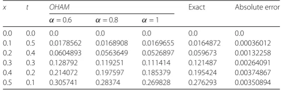
Table 3 Exact and approximate result of Test example4.3with various values ofα

x t OHAM Exact Absolute error

α= 0.6 α= 0.8 α= 1

0.0 0.0 0.0 0.0 0.0 0.0 0.0

0.1 0.5 0.0178562 0.0168908 0.0169655 0.0164872 0.00036012 0.2 0.4 0.0604893 0.0563649 0.0526897 0.059673 0.00132258 0.3 0.3 0.128792 0.119251 0.111414 0.121487 0.00264091 0.4 0.2 0.214072 0.197597 0.185379 0.195424 0.00374867 0.5 0.1 0.305741 0.28374 0.269828 0.276293 0.00350894

with initial condition

Then, considering the first three terms as estimates of solution for Eq. (4.7), we have:

u(x,t)≈

Using the method of least squares, we get

c1= –1.25313, c2= 0.103091.

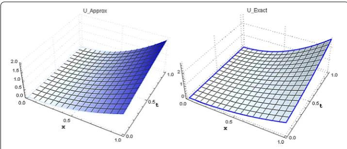
In Table3, we can see the estimated solutions for various values ofα, which are derived for various values of xandtin Fig. 1. We can see the exact and approximate answers featuringα= 1 through applyingOHAM. TheL2_{-norm of the error for Test example4.3}

withα= 1 is 0.020451.

Towardα= 1, the solution we have obtained is in accordance with the exact solution

u(x,t) =x2_exp(t).

Test example4.4 For the fourth instance, consider the FDDEs

Figure 1Comparison of the third-order approximate solution (4.7) with exact solution forα= 1

with initial conditions

u(x, 0) =x, ut(x, 0) = 0. (4.10)

Concerning theOHAM, according to what was formulated and presented in Sect.2, for Eqs. (4.9)–(4.10), we get:

u0(x,t) =x,

u1(x,t) = –

c1xtα α(α),

u2(x,t) =

√

π4–α_c2 1xt2α α(α)(α+1 2)

– c

2 1xtα

(α–α2_)(α)–

c1xtα

(α–α2_)(α)

– c

2 1xtα

(α– 1)(α)–

c1xtα

(α– 1)(α)–

c2xtα α(α), . . . .

Then, considering the first three terms as estimates of solution for Eq. (4.9) we have:

u(x,t)≈x– c1xt

α

(α– 1)(α)–

c1xtα α(α)–

c1xtα

(α–α2_)(α)

–

√

π4–α_c2 1xt2α α(α)(α+1₂)–

c2 1xtα

(α–α2_)(α)+

c2 1xtα

(α– 1)(α)–

c2xtα α(α). Using the method of least squares, by calculations we came to the following:

c1= –1.03557, c2= 0.00250421.

In Table4, we can see the estimated solutions toward various values ofα, which are derived for various values ofxandtby applyingOHAM.

TheL2_{-norm of the error for Test example4.4withα= 2 is 0.000149502.}

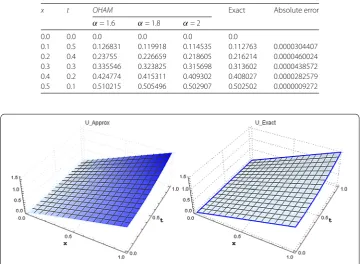
Table 4 Exact and approximate result of Test example4.4with various values ofα

x t OHAM Exact Absolute error

α= 1.6 α= 1.8 α= 2

0.0 0.0 0.0 0.0 0.0 0.0

0.1 0.5 0.126831 0.119918 0.114535 0.112763 0.0000304407 0.2 0.4 0.23755 0.226659 0.218605 0.216214 0.0000460024 0.3 0.3 0.335546 0.323825 0.315698 0.313602 0.0000438572 0.4 0.2 0.424774 0.415311 0.409302 0.408027 0.0000282579 0.5 0.1 0.510215 0.505496 0.502907 0.502502 0.0000009272

Figure 2Comparison of the third-order approximate solution (4.9) with exact solution forα= 2

Test example4.5 For the fifth instance, we consider the system of coupled FDDEs

⎧ ⎨ ⎩

Dα

tu(x,t) +v(x,t) –uxx(x,t) +uvx(x₂,t₂) =₂1(t+ 3x– 2), 0 <α≤1,

Dα

tv(x,t) –u(x2, t 2) +vxx(

x 3,t) +vx(

x 2, 2t) =

1

2(t–x+ 3),

(4.11)

fort> 0 and 0≤x≤1 with initial conditions

u(x, 0) =x, v(x, 0) =x. (4.12)

Forα= 1, the exact solutions areu(x,t) =x–tandv(x,t) =x+t.

With respect to theOHAM, according to what was presented in Sect.2, for Eqs. (4.11)– (4.12), considering the first two terms as estimates of solution for Eq.4.11, we have:

u(x,t)≈x– 11t

α

α(α)+ 3xtα

2α(α)+

tα+1

2(α2_+α)(α)–

10tα

α(α)–

tα+1

2(α2_+α)(α)

+ c1t

α+1

(2α2_{+ 2α)(α)}–

c1tα+1

2(α2_+α)(α)–

10c1tα α(α)+

3c1xtα

2α(α) + t

α+1

(2α2_{+ 2α)(α)}–

√

π41–α_c

1t2α α(α)(α+1₂)–

√

π2–3α–2_c 1xt2α α(α)(α+1₂) +

√

π4–α–1_c 1xt2α α(α)(α+1₂)–

2α–3_c

1x(α+1₂)t3α

√

π α2_(α)(3α) +

11 2–α–2_c

1(2α+ 1)t3α α2_(α)2_{(3α+ 1)}

+ 3c1(α+ 2)t

2α+1

2α(α)(2α+ 3)– 2–α–3_c

1(2α+ 2)t3α+1

Table 5 Exact and approximate result of Test example4.5

x u(x,t) v(x,t)

Approx Exact Absolute error Approx Exact Absolute error

0.25 0.242926 0.24 0.00292615 0.257318 0.26 0.00268185 0.50 0.492925 0.49 0.00292506 0.507322 0.51 0.00267843 0.75 0.742924 0.74 0.00292397 0.757325 0.76 0.00267501 1.00 0.992923 0.99 0.00292287 1.00733 1.01 0.00267159

and

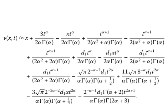
v(x,t)≈x+ 3t

α

2α(α)–

xtα

2α(α)+

tα+1

2(α2_+α)(α)–

tα+1

2(α2_+α)(α)

+ t

α+1

(2α2_{+ 2α)(α)}+

d1tα

2α(α)–

d1xtα

2α(α)–

d1tα+1

2(α2_+α)(α)

+ d1t

α+1

(2α2_{+ 2α)(α)}–

√

π2–α–2_d 1t2α α(α)(α+1₂)+

11√π8–α_d

1t2α α(α)(α+1₂) –3

√

π2–3α–2_d 1xt2α α(α)(α+1₂) –

2–α–1_d

1(α+ 2)t2α+1

α(α)(2α+ 3) . (4.14) Substitutingx= 0.5 andt= 0.5, we getc1= –0.705501 andd1= –0.729647.

In Table 5, we can see the estimated solutions towardα= 1 and t= 0.01, which are derived for various values ofxby applyingOHAM.

5 Conclusion

We have successfully appliedOHAMto obtain approximate solutions of the delay differ-ential equations, delay partial differdiffer-ential equations, and a system of coupled fractional delay equations featuring fractional derivative. The result indicates that a few iterations of

OHAMresult in some useful solutions.

Finally, it should be added that the suggested technique has the potential to be practi-cal in solving other similar nonlinear and linear problems in partial differential equations featuring fractional derivative.

Appendix: Illustration of test example (4.1) in detail

Consider test example (4.1):

Dαu(x) + 2u x

2

u x

2

= 1, 0≤x≤1, 0 <α≤1, (A.1)

with initial condition

u(0) = 0. (A.2)

Considering

u(x,p) =u0+

∞

i=1

and

Equating the coefficients at different powers inp, we have the following differential equa-tions:

The author would also like to thank the office of vice chancellor for research and technology at Islamic Azad University, Qaemshahr branch, Neka branch, and Çankaya University for their financial support.

Funding Not applicable.

Competing interests

The authors declare that they have no competing interests.

Authors’ contributions

All authors contributed equally to the writing of this paper. DB wrote the first draft of a paper; BA did revising and editing; RD was in charge of the choice of the topic, the method, revising, and editing. All three authors read and approved the final manuscript.

Author details

1_{Department of Mathematics, Çankaya University, Ankara, Turkey.}2_{Institute of Space Sciences, Maturely-Bucharest,} Romania. 3_{Department of Mathematics, Qaemshahr Branch, Islamic Azad University, Qaemshahr, Iran.}4_{Department of} Mathematics, Neka Branch, Islamic Azad University, Neka, Iran.

Publisher’s Note

Springer Nature remains neutral with regard to jurisdictional claims in published maps and institutional affiliations.

References

1. Magin, R.L., Abdullah, O., Baleanu, D., Zhou, X.J.: Anomalous diffusion expressed through fractional order differential operators in the Bloch–Torrey equation. J. Magn. Res.190(2), 255–270 (2008)

2. Scalas, E.: The application of continuous-time random walks in finance and economics. Phys. A, Stat. Mech. Appl. 362(2), 225–239 (2006)

3. Deshpande, A.S., Daftardar-Gejji, V., Sukale, Y.V.: On Hopf bifurcation in fractional dynamical systems. Chaos Solitons Fractals98, 189–198 (2017)

4. Neamaty, A., Nategh, M., Agheli, B.: Local non-integer order dynamic problems on time scales revisited. Int. J. Dyn. Control6(2), 486–498 (2018)

5. Raja, M.A.Z., Samar, R., Alaidarous, E.S., Shivanian, E.: Bio-inspired computing platform for reliable solution of Bratu-type equations arising in the modeling of electrically conducting solids. Appl. Math. Model.40(11), 5964–5977 (2016)

6. Guner, O., Bekir, A.: The Exp-function method for solving nonlinear space-time fractional differential equations in mathematical physics. J. Assoc. Arab Univ. Basic Appl. Sci.24, 277–282 (2017)

7. Neamaty, A., Nategh, M., Agheli, B.: Time-space fractional Burger’s equation on time scales. J. Comput. Nonlinear Dyn. 12(3), 031022 (2017)

8. Ming, C., Liu, F., Zheng, L., Turner, I., Anh, V.: Analytical solutions of multi-term time fractional differential equations and application to unsteady flows of generalized viscoelastic fluid. Comput. Math. Appl.72(9), 2084–2097 (2016) 9. Baleanu, D., Luo, A.C.: Discontinuity and Complexity in Nonlinear Physical Systems. Machado, J.T. (ed.). Springer, Cham

(2014)

10. Kilbas, A.A., Srivastava, H.M., Trujillo, J.J.: Theory and Application of Fractional Differential Equations. Elsevier, Amsterdam (2006)

11. Miller, K.S., Ross, B.: An Introduction to the Fractional Calculus and Fractional Differential Equation. Wiley, New York (1993)

12. Doha, E.H., Bhrawy, A.H., Baleanu, D., Hafez, R.M.: A new Jacobi rational-Gauss collocation method for numerical solution of generalized pantograph equations. Appl. Numer. Math.77, 43–54 (2014)

13. Baleanu, D., Magin, R.L., Bhalekar, S., Daftardar-Gejji, V.: Chaos in the fractional order nonlinear Bloch equation with delay. Commun. Nonlinear Sci. Numer. Simul.25(1), 41–49 (2015)

14. Bhalekar, S., Daftardar-Gejji, V., Baleanu, D., Magin, R.: Generalized fractional order Bloch equation with extended delay. Int. J. Bifurc. Chaos22(4), 1250071 (2012)

15. Maraaba, T.A., Jarad, F., Baleanu, D.: On the existence and the uniqueness theorem for fractional differential equations with bounded delay within Caputo derivatives. Sci. China Ser. A, Math.51(10), 1775–1786 (2008)

16. Babakhani, A., Baleanu, D., Khanbabaie, R.: Hopf bifurcation for a class of fractional differential equations with delay. Nonlinear Dyn.69(3), 721–729 (2012)

17. Mohammed, M.J., Ibrahim, R.W., Ahmad, M.Z.: Periodicity computation of generalized mathematical biology problems involving delay differential equations. Saudi J. Biol. Sci.24(3), 737–740 (2017)

18. Jackson, M., Chen-Charpentier, B.M.: Modeling plant virus propagation with delays. J. Comput. Appl. Math.309, 611–621 (2017)

19. Shampine, L.F., Gahinet, P.: Delay-differential-algebraic equations in control theory. Appl. Numer. Math.56(3–4), 574–588 (2006)

20. Mohamadi, A.S., Pourabbas, A., Vaezpour, S.M.: Periodic solutions of delay differential equations with feedback control for enterprise clusters based on ecology theory. J. Inequal. Appl.2014(1), 306 (2014)

21. Graef, J.R., Shen, J.H., Stavroulakis, I.P.: Oscillation of impulsive neutral delay differential equations. J. Math. Anal. Appl. 268(1), 310–333 (2002)

22. Duan, Y., Tian, P., Zhang, S.: Oscillation and stability of nonlinear neutral impulsive delay differential equations. J. Appl. Math. Comput.11(1–2), 243–253 (2003)

23. Milano, F., Dassios, I.: Small-signal stability analysis for non-index 1 Hessenberg form systems of delay differential-algebraic equations. IEEE Trans. Circuits Syst. I, Regul. Pap.63(9), 1521–1530 (2016)

24. Lenz, S.M., Schlöder, J.P., Bock, H.G.: Numerical computation of derivatives in systems of delay differential equations. Math. Comput. Simul.96, 124–156 (2014)

25. Balachandran, B., Kalmár-Nagy, T., Gilsinn, D.E.: Delay Differential Equations. Springer, Berlin (2009)

26. Kajaman, N., Sweilam, N.: Numerical Studies for Fractional-Order Delay Differential Equations. Omniscriptum Gmbh & Company Kg (2016)

27. Moghaddam, B.P., Mostaghim, Z.S.: Modified finite difference method for solving fractional delay differential equations. Bol. Soc. Parana. Mat.35(2), 49–58 (2016)

28. Shakeri, F., Dehghan, M.: Solution of delay differential equations via a homotopy perturbation method. Math. Comput. Model.48(3), 486–498 (2008)

29. Sakar, M.G., Uludag, F., Erdogan, F.: Numerical solution of time-fractional nonlinear PDEs with proportional delays by homotopy perturbation method. Appl. Math. Model.40(13), 6639–6649 (2016)

30. Benhammouda, B., Vazquez-Leal, H.: A new multi-step technique with differential transform method for analytical solution of some nonlinear variable delay differential equations. SpringerPlus5(1), 1723 (2016)

31. Raslan, K.R., Sheer, Z.F.A.: Comparison study between differential transform method and Adomian decomposition method for some delay differential equations. Int. J. Phys. Sci.8(17), 744–749 (2013)

32. Ratib Anakira, N., Alomari, A.K., Hashim, I.: Optimal homotopy asymptotic method for solving delay differential equations. Math. Probl. Eng.2013, Article ID 498902 (2013)

33. Tan, Y., Abbasbandy, S.: Homotopy analysis method for quadratic Riccati differential equation. Commun. Nonlinear Sci. Numer. Simul.13(3), 539–546 (2008)

34. Rashidi, M.M., Abbasbandy, S.: Analytic approximate solutions for heat transfer of a micropolar fluid through a porous medium with radiation. Commun. Nonlinear Sci. Numer. Simul.16(4), 1874–1889 (2011)

35. Abbasbandy, S., Hayat, T., Alsaedi, A., Rashidi, M.M.: Numerical and analytical solutions for Falkner–Skan flow of MHD Oldroyd-B fluid. Int. J. Numer. Methods Heat Fluid Flow24(2), 390–401 (2014)

37. Rahimkhani, P., Ordokhani, Y., Babolian, E.: A new operational matrix based on Bernoulli wavelets for solving fractional delay differential equations. Numer. Algorithms74(1), 223–245 (2017)

38. Heris, M.S., Javidi, M.: On fractional backward differential formulas for fractional delay differential equations with periodic and anti-periodic conditions. Appl. Numer. Math.118, 203–220 (2017)

39. Xu, M.Q., Lin, Y.Z.: Simplified reproducing kernel method for fractional differential equations with delay. Appl. Math. Lett.52, 156–161 (2016)

40. Ali, L., Islam, S., Gul, T., Khan, I., Dennis, L.C.C.: New version of optimal homotopy asymptotic method for the solution of nonlinear boundary value problems in finite and infinite intervals. Alex. Eng. J.55(3), 2811–2819 (2016) 41. Herisanu, N., Marinca, V.: Explicit analytical approximation to large-amplitude non-linear oscillations of a uniform

cantilever beam carrying an intermediate lumped mass and rotary inertia. Meccanica45(6), 847–855 (2010) 42. Gupta, A.K., Ray, S.S.: Comparison between homotopy perturbation method and optimal homotopy asymptotic

method for the soliton solutions of Boussinesq–Burger equations. Comput. Fluids103, 34–41 (2014) 43. Karakoç, F., Bereketo ˇglu, H.: Solutions of delay differential equations by using differential transform method. Int.

J. Comput. Math.86(5), 914–923 (2009)