R E S E A R C H
Open Access
A delayed e-epidemic SLBS model for
computer virus
Zizhen Zhang
1*, Sangeeta Kumari
2and Ranjit Kumar Upadhyay
2*Correspondence:
1School of Management Science and Engineering, Anhui University of Finance and Economics, Bengbu, China
Full list of author information is available at the end of the article
Abstract
We propose an e-epidemic time-delay Susceptible-Latent-Breaking out-Susceptible (SLBS) model to study delay dynamics appearing due to antivirus software, which takes time to clean the viruses from latent and breaking-out computers. We perform nonlinear stability analysis, Hopf bifurcation analysis, and its direction and stability. Numerical simulation results (time series analysis and bifurcation diagram) give useful insights for delay dynamics. We investigate the effect of the control parameters like rate of infection of all the classes and cure rates on the model system. Our results suggest that time delay is responsible for destabilizing the system dynamics. For smooth functionality of a computer system, our results suggest the minimum use of removable storage devices like smart phones, optical discs, memory cards, external hard disk, digital cameras, and so on and use of effective antivirus softwares.
Keywords: Time delay; SLBS model; Computer virus; Stability; Hopf bifurcation
1 Introduction
With increasing popularity of the internet, increasing numbers of network-based applica-tions enter into our everyday life, which can bring about as much as potential hazards mal-ware for network users [1]. Understanding the virus spread dynamics is most important for defence strategies and computer security [2]. In last decades the study of widespread infec-tion of the computers connected to internet has attracted the interest of the researchers at home and abroad. To illustrate the computer virus transmission dynamics, Murray [3] has suggested high similarities between computer and biological viruses. Kephart and White [4,5] investigated SIS models for the spread of computer virus. Wierman [2,6] proposed the SIR computer virus propagation model. Considering that the computer virus has a la-tent period, Yuan et al. [7,8] incorporated the exposed class E (infected but not yet broken-out) to the classical SIR and SEIR computer virus model. However, the SEIR computer virus model assumes that the recovered computers have a permanent immunization pe-riod, which is not consistent with real situation. Mishra and Saini [9] proposed the SEIRS computer virus model to reveal common worm propagation. There are also some other computer virus models with vaccination [10–12], quarantine [13–16], effect of antivirus software [17], and so on.
However, most of the mentioned computer virus models assume that the infected com-puters that are in latency do not infect other comcom-puters. This is not consistent with reality. An infected computer that is in latency can affect other computers during file
ing or copying. Apart from this, new viruses and newer versions of old viruses may infect the cured computers, and effect of removable storage devices are also assumed. Based on these assumptions, the following computer virus model with graded infection rate has been proposed by Yang and Yang [18]:
dS(t)
dt =μ1–
β1L(t) +β2B(t)
S(t) +γ1L(t) +γ2B(t) – (δ+θ)S(t),
dL(t)
dt =μ2+
β1L(t) +β2B(t)
S(t) – (γ1+α+δ)L(t) +θS(t),
dB(t)
dt =αL(t) – (γ2+δ)B(t),
(1)
where S(t), L(t), andB(t) denotes the numbers of uninfected, latent, and breaking-out computers at timet,β1,β2,μ1,μ2,γ1,γ2,δ,α, andθ are the parameters of system (1), and the meanings of all the parameters are the same as those in [18]. Yang and Yang [18] studied the local and global stability of system (1).
Time delay comes from the time sharing of the communication medium and the compu-tation time entailed for communication processing and physical signal coding. The cept of delay comes in the 1970s when analogue controllers were replaced by digital con-trollers in computer networks [19]. Yang [20] demonstrated that the computational delay can cause system instability in a digital controller. Delay is an important aspect because it directly affects the speed of the digital device on an operating computer. In [18] the ef-fect of time delay is not considered; nevertheless, delay acts crucially on system dynamics. Therefore we have deliberated time delay due to the period that antivirus software uses to clean viruses from latent and breaking-out computers. Recently, computer virus models with time delay have been investigated by some scholars [21–26]. In addition to computer virus models with time delay, there are also some other dynamical models with time de-lay, which have shown that time delay causes problems such as instability and restrict the conceivable performance of the control systems. For example, the predator–prey model [27–30], the epidemic model [31–35], and the neural network model [36–39]. All the men-tioned works about delayed dynamical models have shown that time delay can produce complicated nonlinear phenomena with the change of time. Therefore it is important to know that at which time the delay destabilizes the system. Thus we have considered the effect of time delay on the system dynamics. Considering the effect of time delay (denoted asτ) due to the period that antivirus software uses to clean viruses, we investigate the following delayed model:
dS(t)
dt =μ1–
β1L(t) +β2B(t)
S(t) +γ1L(t–τ) +γ2B(t–τ) – (δ+θ)S(t),
dL(t)
dt =μ2+
β1L(t) +β2B(t)
S(t) –γ1L(t–τ) – (α+δ)L(t) +θS(t),
dB(t)
dt =αL(t) –γ2B(t–τ) –δB(t).
(2)
method. In Sect.4, we obtain the stability and direction of Hopf bifurcation by using the theory of center manifold and normal form. Numerical simulation results are presented in Sect.5. Conclusions and discussions are presented in Sect.6.
2 Linear stability and Hopf bifurcation analysis
This section reports the stability analysis of only one existing endemic equilibrium point
E∗ and the critical pointτ0for the local Hopf bifurcation with the help of transversality condition.
Now by direct computation system (2) has a unique endemic equilibrium (S∗,L∗,B∗), where
S∗=μ1+A1B ∗
A2+A3B∗
, L∗=γ2+δ
α B
∗,
andB∗is the unique positive root of the equation
m2
B∗2+m1B∗+m0= 0 (3)
with
m0= –α(μ1θ+μ2δ+μ2θ) < 0,
m1=αδA1+δ(α+γ2+δ)A2–α(μ1+μ2)A3,
m2=δ(α+γ2+δ)A3> 0,
and
A1=
γ1(γ2+δ)
α +γ2, A2=δ+θ, A3=
β1(γ2+δ)
α +β2.
The product of the roots ofB∗ is m0
m2, which is clearly negative, and the discriminant of
Eq. (3) ism2
1– 4m0m2, which is also positive sincem0< 0. Thus Eq. (3) has one positive and one negative root by Vieta’s theorem.
The characteristic equation of system (2) at the endemic equilibrium is
λ3+p2λ2+p1λ+p0+
q2λ2+q1λ+q0
e–λτ+ (r1λ+r0)e–2λτ= 0, (4)
where
p0=a1(a6a7–a5a8) +a4(a2a8–a3a7),
p1=a1(a5+a8) +a5a8–a2a4–a6a7,
p2= –(a1+a5+a8),
q0=a4(a2b4+a8b1–a7b2) –a1(a5b4–a8b3),
q1=b3(a1+a8) +b4(a1+a5) –a4b1,
r0=b4(a4b1–a1b3),
r1=b3b4,
and
a1= –
β1L∗+β2B∗+δ+θ
, a2= –β1S∗,
a3= –β2S∗, a4=β1L∗+β2B∗+θ,
a5=β1S∗– (α+δ), a6=β2S∗,
a7=α, a8= –δ, b1=γ1,
b2=γ2, b3= –γ1,
b4= –γ2.
Forτ= 0, Eq. (4) becomes
λ3+ (p2+q2)λ2+ (p1+q1+r1)λ+p0+q0+r0= 0. (5)
Lemma 2.1 Whenτ= 0,all the roots of Eq. (5)have negative real parts,and the endemic point E∗(S∗,L∗,B∗)of system(2)is locally asymptotically stable(LAS).
Multiplying both sides of Eq. (4) byeλτ, we obtain
q2λ2+q1λ+q0+
λ3+p2λ2+p1λ+p0
eλτ+ (r
1λ+r0)e–λτ= 0. (6)
Forτ> 0, letλ=iω(ω> 0) be the root of Eq. (6). Then
p0+r0–p2ω2
cosτ ω–(p1–r1)ω–ω3
sinτ ω=q2ω2–q0,
p0–r0–p2ω2
sinτ ω+(p1+r1)ω–ω3
cosτ ω= –q1ω.
Thus
cosτ ω= s14ω 4+s
12ω2+s10
ω6+s
04ω4+s02ω2+s00 ,
sinτ ω= s15ω 5+s
13ω3+s11ω
ω6+s
04ω4+s02ω2+s00 ,
(7)
where
s00=p20–r20, s02=p21–r21– 2p0p2, s04=p22– 2p1, s10= –(p0–r0)q0,
s12= (p0–r0)q2– (p1–r1)q1+p2q0, s14=q1–p2q2,
s11= (p1+r1)q0– (p0+r0)q1,
Therefore we obtain the equation
ω12+s5ω10+s4ω8+s3ω6+s2ω4+s1ω2+s0= 0 (8)
with
s0=s200–s210,
s1= 2(s00s02–s10s12) –s211,
s2=s202–s212+ 2(s00s04–s10s14–s11s13),
s3= 2(s00+s02s04–s12s14–s11s15) –s213,
s4=s204–s142 + 2(s02–s13s15),
s5= 2s04–s215.
Now we have (H1): Eq. (8) has at least one positive rootω0. Thus from Eq. (7) we have
τ0= 1
ω0
cos–1
s14ω40+s12ω20+s10
ω06+s04ω40+s02ω20+s00
.
Differentiating Eq. (6) with respect toτ, we obtain
dλ
dτ
–1
= 2q2λ+q1+ (3λ 2+ 2p
2λ+p1)eλτ+r1e–λτ (r1λ2+r0λ)e–λτ– (λ4+p2λ3+p1λ2+p0λ)eλτ
–τ
λ.
Thus we get
dλ
dτ
–1
τ=τ0
=PRQR+PIQI
Q2R+Q2I ,
where
PR=
p1+r1– 3ω20
cosτ0ω0– 2p2ω0sinτ0ω0+q1,
PI=
p1–r1– 3ω20
sinτ0ω0+ 2p2ω0cosτ0ω0+ 2q2ω0,
QR=
p1ω20–r1ω20–ω40
cosτ0ω0–
p2ω30–p0ω0+r0ω0
sinτ0ω0,
QI=
p1ω20+r1ω02–ω40
sinτ0ω0+
p2ω30–p0ω0+r0ω0
cosτ0ω0.
The transversality condition holds if (H2):PRQR+PIQI= 0. We have the following result [25].
Theorem 2.2 Let an endemic point E∗of system(2)exist,and let conditions(H1)and(H2)
be satisfied.Then it is LAS atτ ∈[0,τ0)and unstable forτ>τ0.Furthermore,system(2)
undergoes Hopf bifurcation at E∗whenτ=τ0,and a family of periodic solutions bifurcate
3 Global stability analysis
This section deals with the nonlinear or global stability analysis by constructing suitable Lyapunov function for the endemic equilibrium point of the delayed model system (2).
Theorem 3.1 Ifmin{l1,l2,l3}> 0with
Again, due to form of (14), we consider the functional
whose derivative along the solution of system (2) is given by
D+V11(t)≤D+V1(t) +
where we used the following relation:
ev(t–τ)=ev(t)–
t
t–τ ev(s)dv
LetV2(t) =|v(t)|. Computing the derivative ofV2(t) along the solution of (2), from Eq. (16)
Again, due to the form of (17), we consider the functional
V22(t)≤V2(t) +γ1
whose right derivative along the solution of system (2) is given by
+β2B
where we used the relation
Again, due to the structure of (20), we consider the functional
whose upper right derivative along the solution of system (2) is given by
D+V33(t)≤D+V3(t) +
Let us define the Lyapunov functional
V(t) =V11(t) +V22(t) +V33>u(t)+v(t)+w(t).
–αL∗
Using the mean value theorem, we have
S∗eu(t)– 1=S∗eθ1(t)u(t)>m we conclude that the zero solution of the reduced system (11)–(13) is GAS. Therefore the
endemic equilibriumE∗of model system (2) is GAS.
4 Stability and direction of Hopf bifurcation
In this section, we discuss the stability and direction of Hopf bifurcation using theory of normal form and center manifold [40] of the delayed system (2). Letx1=S–S∗,x2=I–I∗,
x3=T–T∗, andxi(t) =xi(τt) fori= 1, 2, 3. Then the delay system (2) is converted to the following functional differential equation inC=C([–1, 0],R3):
˙
wherex(t) = (x1(t),x2(t),x3(t))T∈C,xt(θ) =x(t+θ),θ∈[–1, 0], andLμ:C→R3,F:R×
C→R3are given by
Lμ(φ) = (τ0+μ)
J1φ(0) +J2φ(–1)
(24)
with
J1=
⎛ ⎜ ⎝
a1 a2 a3
a4 a5 a6 0 a7 a8
⎞ ⎟ ⎠,
J2=
⎛ ⎜ ⎝
0 b1 b2
0 b3 0
0 0 b4
⎞ ⎟ ⎠,
f(μ,φ) = (τ0+μ)
⎛ ⎜ ⎝
–φ1(0)(β1φ2(0) +β2φ3(0))
φ1(0)(β1φ2(0) +β2φ3(0)) 0
⎞ ⎟ ⎠.
(25)
By the Riesz representation theorem there exists a 3×3 matrix-valued functionη(θ,μ) with components of bounded variation forθ∈[–1, 0] such that
Lμφ=
0
–1
dη(θ,μ)φ(θ), ∀φ∈C.
By considering Eq. (24) we can choose
η(θ,μ) = (τ0+μ)
J1δ(θ) +J2δ(θ+ 1)
,
whereδ(θ) is the Dirac delta function. Forφ∈C1([–1, 0],R3), define
A(μ)φ(θ) =
⎧ ⎨ ⎩
dφ(θ)
dθ , θ∈[–1, 0),
0
–1 dη(s,μ)φ(s) =Lμφ, θ= 0,
(26)
and
R(μ)φ(θ) =
⎧ ⎨ ⎩
0, θ∈[–1, 0),
F(μ,φ), θ= 0. Now system (23) becomes
˙
xt=A(μ)xt+R(μ)xt, (27)
wherext(θ) =x(t+θ) forθ∈[–1, 0]. Forψ∈C1([0, 1], (R3)∗), define
A∗(μ)ψ(s) =
⎧ ⎨ ⎩
–dψds(s), s∈(0, 1],
0
and the bilinear inner product
Following the same steps as in [40], we obtain the following expressions:
Solving this system forE1, we obtain
Thus we can compute the following values:
β= 2c1(0)
,
T= –{c1(0)}+μ2{λ (τ
0)}
ω0τ0
,
which determine the properties of a bifurcating periodic solution at the critical valueτ0. The notationsμ,β, andT determine the direction of Hopf bifurcation, stability, and pe-riod of the bifurcating pepe-riodic solutions, respectively. Now we state the results in the following theorem.
Theorem 4.1 Ifμ> 0 (μ< 0),then the Hopf bifurcation is supercritical(subcritical);if
β< 0 (β> 0),then the bifurcating periodic solutions are stable(unstable);if T> 0 (T< 0),
then the periodic solutions increase(decrease).
5 Numerical simulations
Numerical simulation confirms that the delayed system dynamics exhibits a periodic solution for τ > 8.40567. The initial condition throughout the simulation is taken as [10, 5, 5]. The unique endemic equilibriumE∗(16.0404, 29.3064, 14.6532) of system (32) can be obtained by means of Mathematica for the following set of parameter val-ues:
μ1= 4, μ2= 2, α= 0.2,
β1= 0.01, β2= 0.02,
γ1= 0.1, γ2= 0.3,
δ= 0.1, θ= 0.02.
(31)
System (2) becomes
dS
dt = 4 – (0.01L+ 0.02B)S+ 0.1L(t–τ) + 0.3B(t–τ) – 0.12S, dL
dt = 2 + (0.01L+ 0.02B)S– 0.1L(t–τ) – 0.3L+ 0.02S, (32) dB
dt = 0.2L– 0.3B(t–τ) – 0.1B.
From Eq. (5) at τ = 0, we have the characteristic polynomial λ3 +A2λ2 +A1λ+
A0 = 0, whereA0= 0.0395353 > 0, A1= 0.519925, A2 = 1.34572 > 0, andA1A2–A0= 0.66014 > 0. Hence from the set of parameter values given in Eq. (31) we obtain that the endemic equilibrium pointE∗is locally asymptotically stable, which is confirmed by the Routh–Hurwitz criterion.
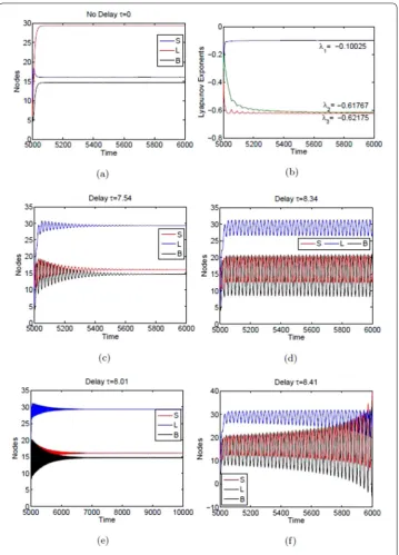
In Fig.1, time series and Lyapunov characteristic exponent (LCE) are performed for ex-ploring system dynamics with and without delay. In absence of delay, the system dynamics is stable for the chosen set of parameters shown in Fig.1(a). A Lyapunov characteristic ex-ponent (LCE) diagram is plotted using Wolf algorithm [41] in absence of delay in Fig.1(b). The value of LCEs (–0.10025, –0.61767, –0.62175) indicates that the system dynamics is stable for the model system (1).
Figure 1(a) Time series without delay, (b) LCE test for (a). Others shows time series of all three classes for different values of time delay. The values of other parameters are same as in (31)
Oscillatory behavior can be seen for the values of time delayτ= 8.34 and 8.41 in Figs.1(d) and1(f ), respectively. From Fig.1(d) we can notice thatτ = 8.34 <τ0; however, it shows oscillatory behavior.
Figure 2The bifurcation diagram of (a) uninfected/susceptible node, (b) latent node, and (c) breaking-out node with respect toτ. The values of other parameters are as in (31)
of τ passes throughτ0= 8.40567, a local Hopf bifurcation occurs, which means that the computer viruses will be out of control and system dynamics will become unsta-ble.
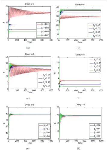
Figure 3Effect of infected rates (β1,β2) on system dynamics (a) uninfected/susceptible node, (b) latent node, and (c) breaking-out node withτ= 8. The values of other parameters are as in (31)
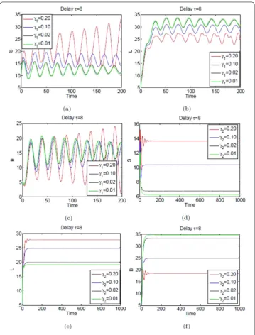
Figure 4Effect of cure rates (γ1,γ2) at which latent and breaking-out computers cured on system dynamics (a) uninfected/susceptible node, (b) latent node, and (c) breaking-out node withτ= 8. The values of other parameters are same as in (31)
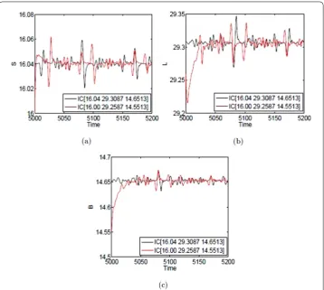
condition leads to a new trajectory and confirms that the system dynamics is chaotic in absence and presence of delay for the proposed system (32).
6 Conclusions and discussions
exper-Figure 5Effect of infected rate at which uninfected computers are infected due to the influence of infected removable storage media (θ) (a) uninfected/susceptible node, (b) latent node, and (c) breaking-out node withτ= 8. The values of other parameters are as in (31)
iments are executed to investigate the dynamics of system (2) and verify the analyt-ical findings for a set of parameter values. Our main results are summarized as fol-lows:
(i) An e-epidemic delayedSLBSmodel for computer virus has been extended to explore the system dynamics. Mainly, the effect of time delay due to the period that the antivirus software uses to clean the viruses in the latent and breaking-out computers has been examined.
(ii) For a given set of parameter values, we obtainA0= 0.0395353 > 0,A1= 0.519925,
A2= 1.34572 > 0, andA2A1–A0= 0.66014 > 0. Hence we concluded that the endemic equilibrium pointE∗(16.0404,29.3064,14.6532) is locally asymptotically stable by the Routh–Hurwitz criterion in absence of delay. The value of Lyapunov exponent confirms the stable system dynamics of the model system (1).
(iii) The bifurcation diagram confirms thatτ0= 8.40567is the critical value for system (32). Whenτ<τ0, the endemic pointE∗is asymptotically stable, and the system is unstable forτ>τ0.
(iv) We obtainc1(0) = 0.00080926 – 0.00164203i,μ= –0.143792 < 0,
Figure 6Time series and SIC test of all three classes without delay. The values of other parameters are as in (31)
subcritical and the bifurcating periodic solutions are unstable with decreasing period.
(v) From Fig.5we observe that as the infected rate at which uninfected computers are infected due to the influence of infected removable storage media (θ) increases, the number of latent and breaking-out computers increases, which is not consistent for smooth functionality of a computer system. Thus we should minimize the use of removable storage media and if necessary, to use it as minimum time as possible because a delay increases the infection probability.
Figure 7Time series and SIC test of (a) uninfected/susceptible node, (b) latent node, and (c) breaking-out node atτ= 8.5. The values of other parameters are as in (31)
Acknowledgements
The authors are grateful to the editor and anonymous referees for their valuable comments and suggestions on the paper.
Funding
This research was supported by Project of Support Program for Excellent Youth Talent in Colleges and Universities of Anhui Province (No. gxyqZD2018044) and the Natural Science Foundation of the Higher Education Institutions of Anhui Province (Nos. KJ2019A0655, KJ2019A0656, KJ2019A0662).
Availability of data and materials
All the authors declare that all the data can be accessed in our manuscript in the numerical simulation section.
Competing interests
The authors declare that there is no conflict of interests.
Authors’ contributions
All authors read and approved the final manuscript.
Author details
1School of Management Science and Engineering, Anhui University of Finance and Economics, Bengbu, China. 2Department of Applied Mathematics, Indian Institute of Technology (Indian School of Mines), Dhanbad, India.
Publisher’s Note
Springer Nature remains neutral with regard to jurisdictional claims in published maps and institutional affiliations.
Received: 19 July 2019 Accepted: 16 September 2019 References
1. Yang, L.X., Yang, X., Wen, L., Liu, J.: A novel computer virus propagation model and its dynamics. Int. J. Comput. Math.
2. Wierman, J.C., Marchette, D.J.: Modeling computer virus prevalence with a susceptible-infected-susceptible model with reintroduction. Comput. Stat. Data Anal.45, 3–23 (2004)
3. Murray, W.: The application of epidemiology to computer viruses. Comput. Secur.7(2), 139–150 (1988) 4. Kephart, J.O., White, S.R.: Directed-graph epidemiological models of computer viruses. In: 1991 IEEE Computer
Society Symposium on Research in Security and Privacy, Oakland, California, pp. 343–359 (1991)
5. Kephart, J.O., White, S.R.: Measuring and modeling computer virus prevalence. In: 1993 IEEE Computer Society Symposium on Research in Security and Privacy, Oakland, California, pp. 2–15 (1993)
6. Piqueira, J.R.C., Araujo, V.O.: A modified epidemiological model for computer viruses. Appl. Math. Comput.213, 355–360 (2009)
7. Yuan, H., Chen, G.Q.: Network virus-epidemic model with the point-to-group information propagation. Appl. Math. Comput.206, 357–367 (2008)
8. Peng, M., He, X., Huang, J.J., Dong, T.: Modeling computer virus and its dynamics. Math. Probl. Eng.2015, Article ID 842614 (2015)
9. Mishra, B.K., Saini, D.K.: SEIRS epidemic model with delay for transmission of malicious objects in computer network. Appl. Math. Comput.188, 1476–1482 (2007)
10. Wang, F.W., Gao, H., Yang, Y., Wang, C.: An SVEIR defending model with partial immunization for worms. Int. J. Netw. Secur.19, 20–26 (2017)
11. Upadhyay, R.K., Kumari, S., Misra, A.K.: Modeling the virus dynamics in computer network with SVEIR model and nonlinear incidence rate. J. Appl. Math. Comput.54, 485–509 (2017)
12. Upadhyay, R.K., Kumari, S.: Global stability of worm propagation model with nonlinear incidence rate in computer network. Int. J. Netw. Secur.20, 515–526 (2018)
13. Nwokoye, C.H., Ozoegwu, G.C., Ejiofor, V.E.: Pre-quarantine approach for defense against propagation of malicious objects in networks. Int. J. Comput. Netw. Inf. Secur.9, 43–52 (2017)
14. Khanh, N.H.: Dynamics of a worm propagation model with quarantine in wireless sensor networks. Appl. Math. Inf. Sci.10, 1739–1746 (2016)
15. Zhao, T., Bi, D.J.: Hopf bifurcation analysis for an epidemic model over the Internet with two delays. Adv. Differ. Equ.
2018, 97 (2018)
16. Liu, J.: Hopf bifurcation in a delayed SEIQRS model for the transmission of malicious objects in computer network. J. Appl. Math.2014, Article ID 492198 (2014)
17. Mishra, B.K., Pandey, S.K.: Effect of antivirus software on infectious nodes in computer network: a mathematical model. Phys. Lett. A376, 2389–2393 (2012)
18. Yang, L.X., Yang, X.F.: A new epidemic model of computer viruses. Commun. Nonlinear Sci. Numer. Simul.19, 1935–1944 (2014)
19. Mahmoud, M.S.: Control and Estimation Methods over Communication Networks. Springer, Berlin (2014) 20. Yang, T.C.: On computational delay in digital and adaptive controllers. In: Control, 1994. Control’94. International
Conference on IET, vol. 2, pp. 906–910 (1994)
21. Feng, L.P., Liao, X.F., Li, H.Q., Han, Q.: Hopf bifurcation analysis of a delayed viral infection model in computer networks. Math. Comput. Model.56, 167–179 (2012)
22. Muroya, Y., Enatsu, Y., Li, H.X.: Global stability of a delayed SIRS computer virus propagation model. Int. J. Comput. Math.91, 347–367 (2014)
23. Upadhyay, R.K., Kumari, S.: Discrete and data packet delays as determinants of switching stability in wireless sensor networks. Appl. Math. Model.72, 513–536 (2019)
24. Ren, J.G., Yang, X.F., Yang, L.X., Xu, Y.H., Yang, F.Z.: A delayed computer virus propagation model with its dynamics. Chaos Solitons Fractals45, 74–79 (2012)
25. Yao, Y., Xie, X.W., Guo, H., Yu, G., Gao, F.X., Tong, X.J.: Hopf bifurcation in an Internet worm propagation model with time delay in quarantine. Math. Comput. Model.57, 2635–2646 (2013)
26. Zhang, Z.Z., Song, L.M.: Dynamics of a delayed worm propagation model with quarantine. Adv. Differ. Equ.2017, 155 (2017)
27. Bai, Y.Z., Li, Y.Y.: Stability and Hopf bifurcation for a stage-structured predator–prey model incorporating refuge for prey and additional food for predator. Adv. Differ. Equ.2019, 42 (2019)
28. Dubey, B., Kumar, A.: Dynamics of prey–predator model with stage structure in prey including maturation and gestation delays. Nonlinear Dyn.96, 2653–2679 (2019)
29. Kundu, S., Maitra, S.: Dynamical behaviour of a delayed three species predator–prey model with cooperation among the prey species. Nonlinear Dyn.92, 627–643 (2018)
30. Kundu, S., Maitra, S.: Dynamics of a delayed predator–prey system with stage structure and cooperation for preys. Chaos Solitons Fractals114, 453–460 (2018)
31. Sirijampa, A., Chinviriyasit, S., Chinviriyasit, W.: Hopf bifurcation analysis of a delayed SEIR epidemic model with infectious force in latent and infected period. Adv. Differ. Equ.2018, 348 (2018)
32. Krishnapriya, P., Pitchaimani, M., Witten, T.M.: Mathematical analysis of an influenza A epidemic model with discrete delay. J. Comput. Appl. Math.324, 155–172 (2017)
33. Xia, W.J., Kundu, S., Maitra, S.: Dynamics of a delayed SEIQ epidemic model. Adv. Differ. Equ.2018, 336 (2018) 34. Liu, Q.M., Sun, M.C., Li, T.: Analysis of an SIRS epidemic model with time delay on heterogeneous network. Adv. Differ.
Equ.2017, 309 (2017)
35. Akimenko, V.: An age-structured SIR epidemic model with fixed incubation period of infection. Comput. Math. Appl.
73, 1485–1504 (2017)
36. Xu, C.J., Liao, M.L., Li, P.L., Guo, Y., Xiao, Q.M., Yuan, S.: Influence of multiple time delays on bifurcation of fractional-order neural networks. Appl. Math. Comput.361, 565–582 (2019)
37. Li, L., Wang, Z., Li, Y.X., Shen, H., Lu, J.W.: Hopf bifurcation analysis of a complex-valued neural network model with discrete and distributed delays. Appl. Math. Comput.330, 152–169 (2018)
38. Xu, C.J., Chen, L., Guo, T., Li, P.L.: Dynamics of FCNNs with proportional delays and leakage delays. Adv. Differ. Equ.
2018, 72 (2018)
40. Hassard, B.D., Kazarinoff, N.D., Wan, Y.H.: Theory and Applications of Hopf Bifurcation. Cambridge University Press, Cambridge (1981)