R E S E A R C H
Open Access
Finite time synchronization problems of
delayed complex networks with stochastic
perturbations
Wenxia Cui
1,2*, Jian-an Fang
2and Shengchao Su
2,3*Correspondence:
1College of Fundamental Studies,
Shanghai University of Engineering Science, Shanghai, 201620, China 2College of Information Science and Technology, Donghua University, Shanghai, 201620, China Full list of author information is available at the end of the article
Abstract
The paper is concerned with the finite-time synchronization problem of delayed complex networks with stochastic perturbations. Based on the finite-time stability theorem, some sufficient conditions are obtained to ensure finite-time
synchronization for the Markovian jump complex networks with time delays and partially unknown transition rates. Finally, the effectiveness of the proposed method is demonstrated by illustrative examples.
Keywords: finite-time; synchronization; stochastic perturbations; complex networks; time delays
Introduction
Over the past decades, the dynamics analysis of complex networks has witnessed rapidly growing research interests since the pioneering work of Watts and Strogatz []. On the one hand, complex networks exist in our daily life with examples including the Inter-net, the World Wide Web, food webs, electric power grids, cellular and metabolic net-works, etc. []. And on the other hand, the dynamical behaviors of complex networks have found numerous applications in various fields such as physics, technology, and the life sci-ences []. In fact, synchronization is a basic motion in nature that has been studied for a long time [–]. Recently, synchronization of complex networks has received increasing research attention [–].
It is important to note that most of the above research results on network synchroniza-tion are based on the asymptotic process of an infinite time. That is, network synchro-nization only occurs when the time tends to infinity. Thus in theory, it is impossible for a network to achieve synchronization in a limited time. However, in actual physical or en-gineering systems, complex networks usually achieve synchronization state in a limited time, which is finite-time synchronization. On the one hand, in the existing literature on finite time synchronization is not treated often. And on the other hand, finite-time syn-chronization is a very important bridge for a complex network to succeed in the actual application. In addition, more and more researchers begin to realize the important role of finite-time synchronization, and there are some related research results [–].
Time delays often occur in complex networks because of the limited speed of signals traveling through the links [] and the frequently delayed couplings in biological neural networks, gene regulatory networks, communication networks, and electrical power grids
[, ]. It has been well known that time delays can cause complex dynamics such as peri-odic or quasi-periperi-odic motions, Hopf bifurcation, and higher-dimensional chaos. It should be noted that [, ] and [] did not consider the time-delay problem. Although there are some works that have been reported on the finite synchronization on delayed networks systems, they are mainly concerned with the finite-time boundedness []. It is checked that the finite-time boundedness is conservative rather than the finite time convergence. In addition, stochastic perturbation becomes one of the main sources for causing insta-bility and poor performance of networks [].
In reality, it has been revealed that a neural network sometimes has finite modes, so that switching from one to another at different times may occur [, ]. And such a switch-ing (or jumpswitch-ing) can be governed by a Markovian chain [, ]. This is partly because a Markovian jump is a suitable mathematical pattern to represent a class of complex net-works subject to random abrupt variations in the structures []. Moreover, Markovian jump complex networks can be regarded as a special class of stochastic network systems. So a great number of significant results on synchronization of Markovian switching net-worked systems have been available in the literature [, , ]. Unfortunately, almost all of the above mentioned works on the synchronization problem of complex networks are built upon the assumption that switching probabilities are known precisely. However, in most cases the transition probabilities of Markovian jump systems or networks are not ex-actly known [–]. Moreover, the estimated values of the mode transition rates may also lead to instability or at least degraded system performance as the partially unknown mode transition rates in system matrices do []. Some extended results concerning the uncer-tain transition probabilities have been reported in [, ]. However, such unceruncer-tainties require the knowledge of a bound or structure of uncertainties, which is conservative to some extent.
Although the finite-time stability or stabilization problems of the control systems has received much attention [, , ], finite-time synchronization of the delayed complex networks has attracted comparatively less attention primarily due to the lack of an ap-propriate control method, and secondly due to the difficulty residing in the mathematical derivation. Besides, how to tackle the coexistence of finite-time synchronization and the other two typical networked-induced constraints, stochastic disturbance and time delays in Markovian jump complex networks with partially unknown transition rates, still re-mains open.
In this paper, finite-time synchronization problems are studied for the delayed com-plex networks with stochastic perturbations and incomplete description of their transi-tion rates. The main features of this paper are twofold: () Based on the finite-time stabil-ity theorem, some sufficient conditions are obtained to ensure finite-time synchronization for the Markovian jump complex networks with time delays and partially unknown tran-sition rates. () For finite-time synchronization research, the model in this paper is more practical, because the network model involves time delays and stochastic perturbations.
Notation Throughout this paper,RnandRn×m denote, respectively, then-dimensional
Euclidean space and the set of alln×mreal matrices. The superscript ‘T’ denotes the
transpose and the notationX≥Y (respectively,X>Y) whereX andY are symmetric
matrices, means thatX–Y is positive semi-definite (respectively, positive definite);Iis
the identity matrix with compatible dimension. · refers to the Euclidean vector norm;
λmin(·) denotes the minimum eigenvalue.diag{· · · }stands for a block-diagonal matrixE. E[x] means the expectation of the random variablex. Matrices, if their dimensions are not explicitly stated, are assumed to be compatible for algebraic operations.
System description and preliminaries
Consider a Markovian switching time-delay complex network composed ofNidentical
nodes with diffusively couplings, in which each node is ann-dimensional delayed
dynam-ical system described by
dxi(t) =
fxi(t),xi(t–τ)
+c
N
j= aij
r(t)xj(t) +ui(t)
dt
+hix(t),x(t–τ),r(t)dωi(t), i= , , . . . ,N ()
where xi(t) = [xi(t),xi(t), . . . ,xin(t)]T∈Rn represents the state vector of the ith node,
τ > is the time delay of node i, f(xi(t),xi(t –τ)) = (f(xi(t),xi(t–τ)),f(xi(t),xi(t–
τ)), . . . ,fn(xi(t),xi(t–τ)))T∈Rnis a continuous vector-valued function, we denotehi(x(t), x(t–τ),r(t)) =hi(x(t),x(t), . . . ,xN(t),x(t–τ),x(t–τ), . . . ,xN(t–τ),r(t))∈Rn×nis the
unknown diffusive coupling matrix. Here,A(r(t)) = (aij(r(t)))N×Ndescribes the linear
cou-pling configuration of the network at timetat moder(t), and is defined asaij(r(t))≥, fori=j,aii(r(t)) = –Nj=,j=iaij(r(t)),i= , , . . . ,N.=diag{γ,γ, . . . ,γn}is the weighted
inner-coupling matrix between nodes, which is positive definite.ui(t) denotes the control
input on the node i,ωi(t) = (ωi(t),ωi(t), . . . ,ωin(t))T is a bounded vector-form Weiner
process that is independent of the Markovian chainr(·), satisfying
Eωij(t) = , E
ωij(t) = , Eωij(t)ωij(s) = (s=t). ()
Let{r(t),t≥}be a right-continuous Markovian process that describes the evolution
of the modes at timetand takes values in the finite spaceS={, , . . . ,r}, with a generator
={πˆiˆj},ˆi,ˆj∈Sgiven by
Pr(t+ t) =ˆj:r(t) =ˆi=
πˆiˆj t+o( t), ifˆj=ˆi,
+πˆiˆj t+o( t), ifˆj=ˆi,
with t> , andlim t→(o( t)/ t) = . Here,πˆiˆj≥ is the transition rate fromˆitoˆjif
ˆ
j=ˆi, whileπˆiˆi= –jˆN=,ˆj=ˆiπˆiˆj.
In this paper, the transition rates of the jumping process are considered to be partly
accessed. For example, the transition rate matrix for network system () withroperation
modes can be expressed as
⎡ ⎢ ⎢ ⎢ ⎢ ⎣
π ? . . . ?
π ? . . . πr
..
. ... . .. ...
? πr . . . πrr
⎤ ⎥ ⎥ ⎥ ⎥ ⎦,
where ‘?’ represents the unknown transition rate. For notational clarity,∀ˆi∈S, we denote
The isolated node (or the uncoupled node) of network () is given by
˙
s(t) =fs(t),s(t–τ),t, ()
wheres(t) = (s(t),s(t), . . . ,sn(t))T∈Rn,s(t–τ) = (s(t–τ),s(t–τ), . . . ,sn(t–τ))T∈Rn.
The diffusive couplings mean that the coupled networks () are decoupled when the systems are synchronized. So, the coupling terms satisfyNj=aij(r(t))s(t) = ,hi(s(t),s(t–
τ),r(t)) = n×n, where n×ndenotes zero matrix ofndimension.
Our control objective is to finite-timely synchronize complex network () to the homo-geneous trajectory (). To reduce the number of controllers, we can adopt the control nodes setJ={l,l+ , . . . ,N}, where <l<N. That is, by adding the suitable designed feed-back controller to complex networks (), there exists a constantt∗> (t∗depends on the initial state vector valuex() = (xT
(),xT(), . . . ,xNT())T), for anyt≥t∗, such that
x(t) =x(t) =· · ·=xN(t) =s(t). ()
Definition The Markovian jump complex network () is said to be synchronization in finite time, if there exists a constantt∗> (t∗ depends on the initial state vector value
x() = (xT
(),xT(), . . . ,xNT())T), for anyt≥t∗, such that
lim
t→t∗
N
i=
Exi(t) –s(t)= , ()
wheres(t) = (s(t),s(t), . . . ,sn(t))T∈Rnis the particular solution of the system ().
Remark In order to fit the model here, we give the definition of [–, , ] as follows:
The complex network () is said to be finite-time synchronization (finite-time boundedness) with respect to(c,c,T)withc<c, if for
≤i<j≤Mxi() –xj()≤c, one has
≤i<j≤M
Exi(t) –xj(t)<c, ∀t∈[,T],i,j= , , . . . ,M.
Obviously, there are differences between the above two definitions, the definition of [– , , ] has more conservatism.
We need the following assumption to study the finite-time synchronization of the com-plex network ().
Assumption There exist two constant matrices= (θij)n×nand= (ϕij)n×n, in which
θij≥,ϕij≥, such that
fit,x(t),x(t–τ)–fit,y(t),y(t–τ)
≤
n
j=
θijxj(t) –yj(t)+ϕijxj(t–τ) –yj(t–τ), ()
By Assumption , define the following parameters:
¯
a= max
≤μ≤n
n
ν=
θμν+ϕμν +θνμ(–), b¯= max
≤μ≤n
n
ν=
ϕνμ(–),
where∈[, ].
Assumption There exist nonnegative constantsξijˆi,ηijˆi,i,j= , , . . . ,N, such that
traceh˜Ti e(t),e(t–τ),r(t)h˜i
e(t),e(t–τ),r(t) ≤
N
j=
ξijˆieTi (t)ei(t) +ηijiˆeTi(t–τ)ei(t–τ), ()
wherehi˜(e(t),e(t–τ),r(t)) =hi(x(t),x(t–τ),r(t)) –hi(s(t),s(t–τ),r(t)),r(t) =ˆi∈S,ei(t) =
xi(t) –s(t),ei(t–τ) =xi(t–τ) –s(t–τ).
Assumption [] Let <β< andλ> , there exists a continuous functiong: [,∞)→ [,∞) withg() > , for any ≤u≤t, such that
g(t) –g(u)≤–λ
t
u
gβ(s)ds. ()
Assume that the initial condition of the network () is given by
xi(z) =ϕi(z)∈C
[–τ, ],Rn, i= , , . . . ,N,
whereC([–τ, ],Rn) denotes the set of continuous functions mapping the interval [–τ, ]
intoRn.
Before ending this section, let us recall the following results, which will be used in the next section.
Lemma (Finite-time stability theorem []) Suppose that function V(t) : [,∞)→
[,∞) is differentiable (the derivative of V(t) at is in fact its right derivative) and dV(t)
dt ≤–ηV
β(t), whereη> and <β < .Then V(t) will reach zero at finite time
t∗≤V–β()/(η( –β))and V(t) = for all t≥t∗.
Lemma (Jesen inequality []) If a,a, . . . ,anare positive number and <α<β,then
(ni=aβi)β ≤(n i=aαi)
α.
Lemma [] Ifξ,ξ, . . . ,ξn≥and <p≤,then(ni=ξi)p≤ni=ξ p i.
Main results
theo-rem, sufficient conditions for the finite-time synchronization control problems are de-rived.
We present the finite-time synchronization criterion to ensure that a delayed complex network can be pinned. Subtracting () from (), we obtain the following error dynamical systems:
˙
ei(t) =F
ei(t),ei(t–τ)
+c
N
j=
aˆiijej(t) +ui(t)
+h˜i
e(t),e(t–τ),ˆidωi(t), i= , , . . . ,N,ˆi∈S, ()
whereF(ei(t),ei(t–τ)) =f(xi(t),xi(t–τ)) –f(s(t),s(t–τ)),h˜i(e(t),e(t–τ),ˆi) =hi(x(t),x(t–
τ),ˆi) –hi(s(t),s(t–τ),ˆi),ei(t) =xi(t) –s(t).
For the coupled system (), we use the following linear negative feedback controllers:
ui(t) = –εˆiiei(t) –kˆiisign
ei(t)ei(t)
β
, ()
whereεˆii> andkˆii> ,i∈J, otherwise,εiˆi=kiiˆ= ,i∈/J,ˆi∈S.|ei(t)|β= (|ei
(t)|β,|ei(t)|β,
. . . ,|ein(t)|β)T and sign(·) is the sign function, sign(ei(t)) = diag{sign(ei
(t)),sign(ei(t)),
. . . ,sign(ein(t))}, the real numberβsatisfies <β< ,i= , , . . . ,N.
In view of the pinning algorithm (), we apply a pinning controller to the network () such that the network () has finite-time synchronization in the finite time. We obtain the following error dynamical systems:
˙
ei(t) =F
ei(t),ei(t–τ)
+c
N
j=
aˆiijej(t) –εiiˆei(t) –kiˆisign
ei(t)ei(t)
β
+h˜i
e(t),e(t–τ),ˆidωi(t), i= , , . . . ,N, ()
where εiˆi > and kiˆi > , i ∈J, otherwise, εiˆi=kiiˆ = , i ∈/ J, ˆi∈S. F(ei(t),ei(t–τ)) =
f(xi(t),xi(t–τ)) –f(s(t),s(t–τ)),ei(t) =xi(t) –s(t).
Theorem Let Assumptions-hold.If
⎧ ⎪ ⎪ ⎪ ⎪ ⎨ ⎪ ⎪ ⎪ ⎪ ⎩
(–σ+a¯+πˆi)IN+ˆi λmin() + cA
ˆ
i– ϒˆi≤,
ˆi– ( –σ–b¯)IN ≤, qˆj–δˆi≤, ifjˆ=ˆi,ˆj∈S, qˆj–δˆi≥, ifˆj=ˆi,ˆj∈S,
()
whereϒˆi=diag{, . . . ,
l
,εˆli+, . . . ,εNiˆ } ∈RN×N is the diagonal matrix, πˆi=
ˆ j∈Sˆi
πˆiˆj(qˆj–
δˆi)/qˆi(δˆi> ,qˆi> ), <σ< ,then,under the set of controllers(),the complex network
()is synchronization at finite time
t∗≤τ+V(,r())
–+β
where <β< ,γ =min(k,λσ),k=mini,ˆi(kiˆi),i∈J,iˆ∈S.V(,r()) =qr()
N
i=eTi()ei(), ei()is the initial condition satisfying Assumption.
Proof Forˆi∈S, design the stochastic Lyapunov-Krasovskii functionalV(t,e(t),ˆi) as
fol-LetLV (see [], the generalized Itô formula) denote the second-order differential
op-erator ofV with respect to () defined by
Assumption , the following inequality is obtained:
It follows from the inequalities ()-() that
+qˆieT(t–τ)
Denoteγ=min(k,λσ), by Lemma , the following inequalities are given:
k
Taking the expectation on both sides of (), from () we get
ELVt,e(t),ˆi ≤E According to the Definition , the coupled complex network () is finite-time
synchroniza-tion in the finite timet∗. The proof is hence completed.
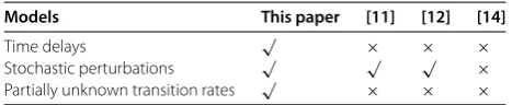
Table 1 Model comparisons
Models This paper [11] [12] [14]
Time delays √ × × ×
Stochastic perturbations √ √ √ ×
Partially unknown transition rates √ × × ×
Here ‘√’ means that the model contains this component, ‘×’ means that the model does not contain this component.
Remark [–, , ] Investigated the finite-time boundedness synchronization problems for complex networks with time delays. Different from this literature, this paper studied the network synchronization to achieve in a finite time. Therefore, the result of this paper shows more advantages.
WhenA(r(t)) =A, and we use the following linear negative feedback controllers:
ui(t) = –εiei(t) –kisign
ei(t)ei(t)β, ()
where εi > , ki > , i∈J, otherwise, εi =ki = , i∈/ J. |ei(t)|β = (|ei(t)|β,|ei(t)|β, . . . ,
|ein(t)|β)T,i= , , . . . ,N. We can obtain the following corollary.
Corollary Let Assumptionsandhold.If
(–σ+a¯)I N
λmin() + cA– ϒ≤,
–σ–b¯≥, ()
whereϒ=diag{, . . . ,
l
,εl+, . . . ,εN} ∈RN×N is the diagonal matrix, <l<N, <σ< , then,under the set of controllers(),the complex network() (A(r(t)) =A)is
synchroniza-tion at finite time t∗≤τ +V()– +β
γ(–+β),where <β< ,γ =min(k,λσ),and k=mini(ki), i∈J.V() =Ni=eT
i ()ei(),ei()is the initial condition satisfying Assumptionof ei(t) = xi(t) –s(t),i= , , . . . ,N.
Numerical examples
In this section, the example is given to demonstrate the effectiveness of the proposed ap-proach.
Example Consider the following Markovian jumping time-delay complex network:
˙
xi(t) =fxi(t),xi(t–τ)+c
j=
aˆiijxj(t) +ui(t)
+hix(t),x(t–τ),r(t)dωi(t), ()
wherexi(t) = (xi(t),xi(t))Tis the state variable of theith node,i= , , ,ˆi= , , , ,τ= , c= ,=diag{, .}. We choose control nodes setJ={, }. We have
A= ⎡ ⎢ ⎣
– . .
. – .
. . –.
⎤ ⎥
⎦, A= ⎡ ⎢ ⎣
–. . .
. –. .
. . –
A=
The partially transition rate matrix is given by
⎡
network (). Now we verify that the condition () in Assumption is satisfied. Fori=
, , , lethˆii(t,x(t),xi(t–τ)) = .ˆidiag{¯xi,xi¯}, wherexi¯=xi(t) +xi(t–τ) – (xi+,(t) +
applying Theorem to this example and the following feasible solutions can be obtained:
σ= . and
ϒ=diag{, ., .}, ϒ=diag{, ., .},
ϒ=diag{, ., .}, ϒ=diag{, ., .}.
The initial conditions of the numerical simulations are taken as:x() = (–., –.)T, x() = (–., .)T,x() = (., –.)T. Through a simple computation, we getV() =
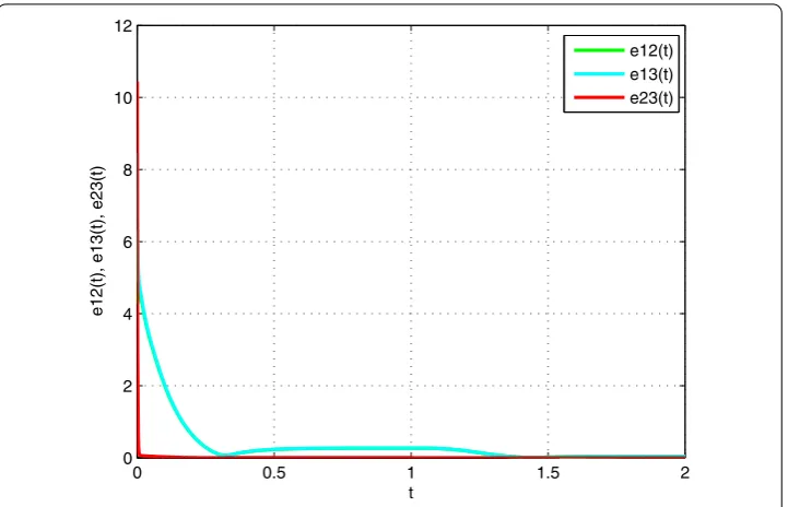
To further verify the effectiveness of the proposed control design for Example , Figure describes the time response of the state errors variablese(t),e(t),e(t), which implies
Figure 1 Time response of the error variablese12(t),e13(t),e23(t) for Example 1.
Conclusions
This paper has introduced a general delayed complex networks model with stochastic per-turbations and the finite-time synchronization problem of Markovian switching complex networks with stochastic disturbance. Based on the finite-time stability theorem and in-equality technique, easily testable conditions have been established to ensure finite-time synchronization for the addressed complex networks. Moreover, conditions that guaran-tee the finite-time synchronization of the delayed complex networks without switching have also been established. With variable time delays or random delays or mixed delays, finite-time synchronization research of Markovian switching complex network remains open. And it is hard for us to solve such problems, which is our future research.
Competing interests
The authors declare that they have no competing interests.
Authors’ contributions
All authors contributed equally to the writing of this paper. All authors read and approved the final manuscript.
Author details
1College of Fundamental Studies, Shanghai University of Engineering Science, Shanghai, 201620, China.2College of
Information Science and Technology, Donghua University, Shanghai, 201620, China. 3Modern Industry Training Center, Shanghai University of Engineering Science, Shanghai, 201620, China.
Acknowledgements
The work was supported by the Education Commission Scientific Research Innovation Key Project of Shanghai under Grant 13ZZ050, the Science and Technology Commission Innovation Plan Basic Research Key Project of Shanghai under Grant 12JC1400400.
Received: 10 November 2013 Accepted: 20 March 2014 Published:19 May 2014 References
1. Watts, DJ, Strogatz, SH: Collective dynamics of small-world. Nature393, 440-442 (1998)
2. Li, H: Synchronization stability for discrete-time stochastic complex networks with probabilistic interval time-varying delays. Int. J. Innov. Comput. Inf. Control7, 697-708 (2011)
4. Wu, Z, Shi, P, Su, H, Chu, J: Sampled-data synchronization of chaotic Lur’e systems with time delays. IEEE Trans. Neural Netw. Learn. Syst.24, 410-421 (2013)
5. Wu, CW, Chua, LO: A unified framework for synchronization and control of dynamical systems. Int. J. Bifurc. Chaos4, 979-998 (1994)
6. Lü, J, Yu, X, Chen, G: Synchronization of general complex dynamical networks. Physica A334, 281-302 (2004) 7. Tang, Y, Wong, WK: Distributed synchronization of coupled neural networks via randomly occurring control. IEEE
Trans. Neural Netw. Learn. Syst.24, 435-447 (2013)
8. Wu, Z, Shi, P, Su, H, Chu, J: Stochastic synchronization of Markovian jump neural networks with time-varying delay using sampled data. IEEE Trans. Cybern.43, 1796-1806 (2013)
9. Zhang, W, Tang, Y, Fang, J, Zhu, W: Exponential cluster synchronization of impulsive delayed genetic oscillators with external disturbances. Chaos21, 043137 (2011)
10. Yang, X, Cao, J, Lu, J: Synchronization of Markovian coupled neural networks with nonidentical node delays and random coupling strengths. IEEE Trans. Neural Netw. Learn. Syst.1, 60-71 (2012)
11. Yang, X, Cao, J: Finite-time stochastic synchronization of complex networks. Appl. Math. Model.34, 3631-3641 (2010) 12. Sun, Y, Li, W, Zhao, D: Finite-time stochastic outer synchronization between two complex dynamical networks with
different topologies. Chaos22, 023152 (2012)
13. Ma, Q, Wang, Z, Lu, J: Finite-time synchronization for complex dynamical networks with time-varying delays. Chaos
22, 043151 (2012)
14. Chen, Y, Lü, J: Finite-time synchronization of complex dynamical networks. J. Syst. Sci. Complex.29, 1419-1430 (2009) 15. Hou, L, Zong, G, Wu, Y: Finite-time control for switched delay systems via dynamic output feedback. Int. J. Innov.
Comput. Inf. Control8, 4901-4913 (2012)
16. Cui, W, Fang, J, Zhang, W, Wang, X: Finite-time cluster synchronization of Markov switching complex networks with stochastic perturbations. IET Control Theory Appl.8, 30-41 (2014)
17. Yuan, C, Mao, X: Robust stability and controllability of stochastic differential delay equations with Markovian switching. Automatica40, 343-354 (2004)
18. Wu, Z, Shi, P, Su, H, Chu, J: Passivity analysis for discrete-time stochastic Markovian jump neural networks with mixed time delays. IEEE Trans. Neural Netw.22, 1566-1575 (2011)
19. Zhang, L, Boukas, E, Lam, J: Analysis and synthesis of Markov jump linear systems with time-varying delays and partially known transition probabilities. IEEE Trans. Autom. Control53, 2458-2464 (2009)
20. Du, B, Lam, J, Zou, Y, Shu, Z: Stability and stabilization for Markovian jump time-delay systems with partially unknown transition rates. IEEE Trans. Circuits Syst. I, Regul. Pap.60, 341-351 (2013)
21. Zhang, Y, He, Y, Wu, M, Zhang, J: Stabilization for Markovian jump systems with partial information on transition probability based on free-connection weighting matrices. Automatica47, 79-84 (2011)
22. Xiong, J, Lam, J, Gao, H, Ho, D: On robust stabilization of Markovian jump systems with uncertain switching probabilities. Automatica41, 897-903 (2005)
23. Shu, Z, Lam, J, Xu, S: Robust stabilization of Markovian delay systems with delay-dependent exponential estimates. Automatica42, 2001-2008 (2006)
24. Yin, J, Khoo, S, Man, Z, Yu, X: Finite-time stability and instability of stochastic nonlinear systems. Automatica47, 2671-2677 (2011)
25. Bhat, SP, Bernstein, DS: Finite-time stability of continuous autonomous systems. SIAM J. Control Optim.38, 751-766 (2000)
26. Xu, L, Wang, X: Mathematical Analysis Methods and Examples, pp. 36-37. Higher Education Press, Beijing, China (1983)
27. Wang, L, Xiao, F: Finite-time consensus problems for networks of dynamic agents. IEEE Trans. Autom. Control55, 950-955 (2010)
28. Gilli, M: Strange attractors in delayed cellular neural networks. IEEE Trans. Circuits Syst. I, Fundam. Theory Appl.40, 849-853 (1993)
10.1186/1687-1847-2014-149