Analysis and Comparison of Algorithms for
Training Recurrent Neural Networks
Diploma Thesis by
Ulf D. Schiller
Supervised by
Dr. Jochen J. Steil Prof. Dr. Helge Ritter
The Neuroinformatics Group Faculty of Technology University of Bielefeld
How did that work? No need to concern myself; the majority of people benefit from the technology of their civilization without understanding it.
Return from the Stars
iii
Contents
1 Introduction 1
2 Artificial Neural Networks 4
2.1 Computational Neurons . . . 4
2.2 Neural Networks . . . 6
2.2.1 Feedforward Neural Networks . . . 6
2.2.2 Recurrent Neural Networks . . . 7
2.3 Learning and Error Propagation . . . 9
2.3.1 Credit Assignment and Gradient Descent . . . 10
2.3.2 Online vs. Batch Learning . . . 10
2.3.3 Generalization and Overfitting . . . 11
2.3.4 Error Propagation in Feedforward Networks . . . 11
2.3.5 Error Propagation in Recurrent Neural Networks . . . 12
2.4 Atiya-Parlos Recurrent Learning (APRL) . . . 14
2.4.1 Batch Update . . . 15
2.4.2 Online Update . . . 16
2.4.3 Interpretation of the Algorithm . . . 16
2.5 Real-Time Recurrent Learning (RTRL) . . . 18
2.6 Echo State Networks . . . 18
2.7 Stability of Neural Networks . . . 20
3 The Training Setup 23 3.1 The Roessler Attractor . . . 23
3.2 The Network Architecture . . . 24
4 Recurrent Learning: APRL vs. RTRL 26 4.1 Real-Time Recurrent Learning of the Roessler Attractor . . . 26
4.2 Atiya-Parlos Recurrent Learning of the Roessler Attractor . . . 32
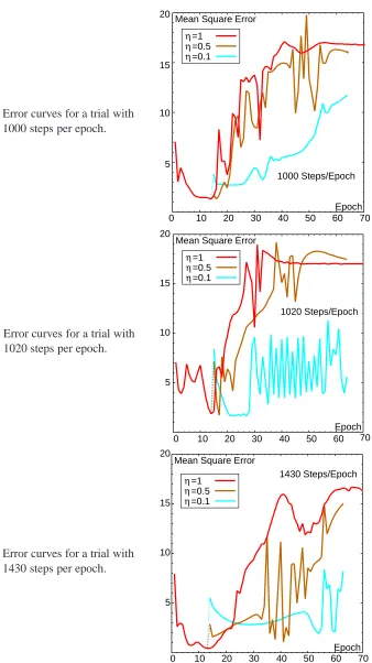
4.3 Reducing the Learning Rate . . . 37
4.4 Learning with Smaller Learning Rates . . . 41
5 Analyzing the Weight Dynamics of Recurrent Learning 44 5.1 The One-Output-Behavior of the Atiya-Parlos Algorithm . . . 44
5.2 Comparison with Echo State Networks . . . 47
5.3 Weight Change for Atiya-Parlos Recurrent Learning . . . 48
5.4 Weight Change for Real-Time Recurrent Learning . . . 51
5.5 Initialization of the Reservoir . . . 53
5.5.1 Initialization with Positive Bias . . . 53
5.5.2 Initialization with Scaled Columns . . . 53
5.5.3 Initialization with Large Weights . . . 54
5.6 Algorithm Switching with Weight Exchange . . . 56
iv
5.6.2 Switching from RTRL to APRL . . . 61
6 Aspects of Stability 65 6.1 Tracing Fixed Points . . . 65
6.2 Stability Analysis for Real-Time Recurrent Learning . . . 67
6.3 Stability Analysis for Atiya-Parlos Recurrent Learning . . . 71
6.4 Conclusions . . . 74
7 Perspectives on new Algorithms 75 7.1 Hybrid Batch-Online APRL . . . 75
7.2 Accelerated One-Output APRL . . . 77
7.3 Other Optimization Methods . . . 77
8 Summary and Conclusive Remarks 79 A Methods from Matrix Algebra 83 A.1 Pseudoinverse Matrices . . . 83
A.2 The Small Rank Adjustment Matrix Inversion Lemma . . . 84
B Details for the Derivation of the Atiya-Parlos Algorithm 86 B.1 Matrices for the Unified Formulation of Gradient Descent . . . 86
B.2 Derivation of the Matrix Notation of the Atiya-Parlos Learning Rule . . . 87
C Tables 89
Bibliography 101
1
1
Introduction
Neural networks are nowadays a well established computational approach to solving complex tasks. The term “neural networks” originates from the analogy to the networks of biological neurons in the nervous system of animals. In contrast to the idea of computing as executing a stored program of serial manipulations of symbolic representations, neural networks are inspired by the parallel and distributed information processing in the brain. Single neurons are connected to each other and interactions between different units of the brain can take place to exchange messages or to access results. From the high complexity of these mechanisms, the cooperative phenomena emerge which we subsume under the term “intelligence”. The attempt to emulate these capabilities in computational models has led to the connectionist paradigm in artificial intelligence research.
A first model of a neuron was introduced by McCulloch and Pitts [1943] and is made up of a discrete time linear threshold unit. It implements the basic features of biological neurons such as synaptic summation, threshold and firing. McCulloch-Pitts neurons suffice to construct neural networks that can perform arbitrary complex computations. A more realistic model is based on the Hodgkin-Huxley equations [Hodgkin and Huxley, 1952], which describe the time course of the spike activity of biological neurons. The result are leaky-integrator neurons that act on a continuous time scale. The spike frequency is approximated by an activation function, which is usually of sigmoidal shape. Leaky integrator neurons are thus nonlinear units, and as continuous time units they are suitable for modeling temporal effects.
The relatively simple neurons are used as building blocks for neural networks. The interconnec-tions between single neurons allow for the propagation of activities through the network, which as a whole implements a complex information processing system. Two basic types of neural networks are distinguished according to the structure of interconnections: feedforward neural networks and recurrent neural networks. Feedforward networks are structured into layers and have no loops. The activity is propagated layer by layer from the input to the output. Such networks were initially studied by Rosenblatt [1958] under the name perceptrons. Probably the most widely known feed-forward networks are multilayer perceptrons. They represent static input-output mappings and are capable of approximating any function with arbitrary precision [Funahashi, 1989].
Recurrent neural networks are networks with arbitrary connections between its neurons. Feed-back connections give rise to cyclic activity propagation. Hence the output of the network is not only dependent on the current input, but also on the internal states, which again are dependent on previous inputs. In this way, the internal states represent a kind of memory that stores the past course of the inputs. The recurrent neural network thus transforms an input sequence into an out-put sequence. This capability makes them attractive for application in sequence recognition and sequence generation tasks.
2 1 Introduction
that a recurrent neural network can approximate any dynamics on a compact set and finite time horizon with arbitrary precision [Funahashi and Nakamura, 1993]. However, the problem in the application of recurrent neural networks is that they can exhibit unstable behavior which is hard to predict. Only in the restricted case of networks with symmetric connections, convergence to a stable state can be guaranteed [Hopfield, 1982]. Therefore ongoing effort is spent on the analysis of the dynamical behavior of recurrent neural networks.
The key to the computational power of neural networks is the possibility to adapt them to a certain task. Inspired by the synaptic plasticity of the brain, the connection weights of the neural network are considered to be adjustable parameters. The appropriate parameters are determined by “learning” or “training” the desired task from a set of input-output examples. No explicit knowledge of the underlying rules of the task is necessary because the network may infer the relevant dependencies from the example data.
The procedure to find the parameters is often based on minimizing some error measure that indicates the deviation of the networks current output from the desired output. The problem is to relate the deviation to a certain connection weight that is responsible for the error and should be updated. It is known as the credit assignment problem and has to facets: The structural credit assignment problem concerns the difficulty to assign the output error to weights inside the network structure. The temporal credit assignment problem raises the question how the error at one time can be accounted for in the weight updates at later times.
A mathematical technique for the purpose of minimizing the error measure is gradient descent. Based on gradient descent, Rumelhart, Hinton, and Williams [1986] were able to derive a learning rule which solves the credit assignment problem for feedforward networks. The error is backprop-agated from the outputs through the entire network to the input connections. Every weight update is calculated according to the location of the respective weight in the network. Together with this learning rule, multilayer perceptrons have been successfully used in various applications.
For recurrent neural networks, a learning rule is more complicated to derive because the er-roneous output is fed back into the network over the connections and influences future network states. This makes it difficult to relate the error to weights of a certain neuron. Moreover, the weight updates can also change the future behavior of the network. Learning algorithms that take into account the dynamic character of recurrent networks have first been proposed for special ar-chitectures [Jordan, 1986; Elman, 1990]. Other approaches try to generalize backpropagation to recurrent networks. For networks that reach a stable state, this led to the recurrent backpropaga-tion algorithm [Pineda, 1987; Almeida, 1987]. Well known gradient based algorithms for arbitrary recurrent networks are backpropagation through time (BPTT) [see Werbos, 1990] and real-time recurrent learning (RTRL) [Williams and Zipser, 1989; Pearlmutter, 1995].
However, these algorithms are computationally expensive. In addition they are not suited for learning tasks with long-term dependencies because they suffer from the vanishing gradient problem [Hochreiter, 1998]. Approaches to overcome this sometimes make use of regularization techniques that apply certain restrictions to either the architecture of the neural network or to the learning algorithm [see Hammer and Steil, 2002, for a review].
Many of the gradient based algorithms were brought to a unified formulation by Atiya and Par-los [2000] by regarding the learning procedure as a constrained optimization problem. The novel formulation was also used to derive a new algorithm, Atiya-Parlos recurrent learning (APRL), that improves the complexity toO(N
3
In this work, I will analyze and compare algorithms for training recurrent neural networks. Special emphasis will lie on the recent Atiya-Parlos algorithm. The aim is to get insights in the behavior of the algorithms and how it is related to the strategy of minimizing the output error. The Atiya-Parlos algorithm is based on computing a different gradient of the error functional than other algorithms. The question arises whether this approach is equally feasible for training recurrent networks. To answer this, the Atiya-Parlos algorithm is compared to real-time recurrent learning on the task of learning the Roessler attractor.
The weight space in which the algorithms search is high-dimensional, and it is therefore very difficult to describe the structure of this space. A characterization of the structure of the weight space and the location of minima of the error could lead to a deeper understanding of algorithms and to future improvements. Maybe some aspects can be revealed by analyzing the strategy used by the algorithms to navigate through the weight space. This will be investigated by observing the weight dynamics of the different algorithms.
Another important aspect in training recurrent neural networks is how the weight changes affect the stability of the neural network. There are approaches available how stability can be incorporated into the learning process [see for example Steil and Ritter, 1999a]. However, it remains an interesting question how stability of the network is influenced by the weight updates. An attempt to answer it is made by tracing the fixed points of the network during the training process.
The remainder of this work is organized as follows: In chapter 2, the theoretical background of artifical neural networks that is needed in this work is presented. After introducing neurons and neural networks, the foundations of training neural networks are explained. In particular, the continuous time version of the Atiya-Parlos algorithm is derived and real-time recurrent learning and echo state networks are reviewed. In addition, the basic notions of stability are introduced.
In chapter 3, the training setup used in this work is described. The Roessler attractor is intro-duced, whose flow implicitly defines the input-output function that is to be learned by the network. Subsequently, the details of the training procedure are described.
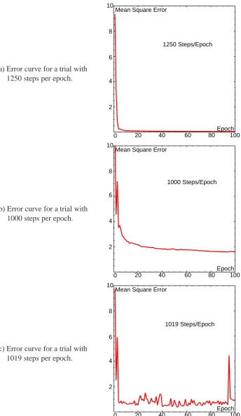
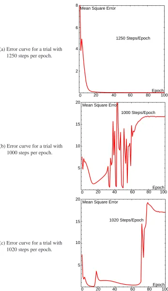
The results obtained by learning with RTRL and APRL are presented in chapter 4. The training and generalization errors of the trained networks are discussed with respect to the properties of the algorithms. The results reveal that APRL often shows an error overshoot after reaching the minimal training error. Further simulations are carried out with variable learning rates, which indicate that the overshoot is unavoidable.
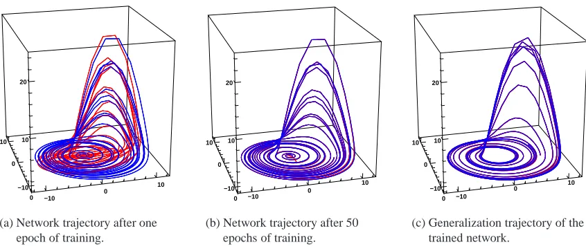
Chapter 5 deals with the weight dynamics of recurrent learning. A formal analysis of the one-output behavior of APRL is conducted, which shows that the network is highly structured. This result is compared with the related approach of echo state networks. Then the weight dynamics of APRL and RTRL is compared in experiments. The relevance of the initialization of the weights for the performance of APRL is investigated. Finally, it is investigated whether the learning per-formance can be improved by mutually exchanging the weight matrices and continuing to adapt them with the other algorithm.
In chapter 6, the stability of the networks is analyzed. A technique to trace fixed points is developed and applied to APRL and RTRL. Some examples of how the results can look like are presented.
Finally, chapter 7 sketches some perspectives how new algorithms can be developed based on the special weight dynamics of APRL. Two variants of APRL are proposed, which however have not been tested yet.
4 2 Artificial Neural Networks
2
Artificial Neural Networks
In the following, the foundations of neural computation are reviewed. Though biological aspects are used to motivate some concepts, the focus is on the computational aspects of neural networks. Computing with artificial neural networks or – in terms of Hertz et al. [1991] – “network compu-tation” is used both in computational neuroscience and neural computation. Some authors prefer to use distinct vocabulary to match those fields. In this work, I will not be that rigorous and use terms like “neuron”, “unit” or “node” as synonyms.
The perspective in which neural networks are presented here is to view them as adaptive
dynamical systems. After introducing the basic building blocks for neural networks, the main
types of neural networks are presented. Then a general approach to adapting a neural network to a certain task is given and some important algorithmic techniques are derived. Finally, the basic concepts concerning stability of neural networks as dynamic systems are summarized.
2.1
Computational Neurons
The basic unit in the brain is the neuron. There is a variety of different types of biological neurons, which differ in aspects like location, function, form or the mechanisms of signal transmission. Neural computation is based on modeling the properties of biological neurons by computational units. Abstracting from the more specific properties, a basic neuron can be outlined as follows: The incoming signals are collected at the dendrites which are connected as ramifications to the cell body (soma). At the soma, all inputs to the cell surface are accumulated. From the cell body, a single long strand (the axon) extends and branches into the axonal arborization. The ends of the branches form connections to other neurons, called synapses. The mechanism of signal transmission is a combination of complex electrical and chemical processes. Basically, the soma performs a synaptic summation of all signals received at its surface. If the sum exceeds a certain threshold, an output signal is triggered that propagates as an action potential (spike) along the axon. This process is called firing. When the spike arrives at a synapse, a chemical substance (transmitter) is released that can lead to an input signal at the dendrites of another neuron.
A simple computational model of a neuron was introduced by McCulloch and Pitts [1943].
Definition 2.1 (McCulloch-Pitts neuron) A McCulloch-Pitts neuron is a computational unit with
n2Ninputsu
j, weights w
j, a threshold
and outputx(j=1;:::;n). It operates on a discrete time scalet=0;1;2;3;:::. The output at time step t+1 is one, if the weighted sum of the inputs at timetexceeds a threshold, and zero otherwise:
x(t+1)= 0
@ n X
j=1 w
j u
j (t)
1
A
; (2.1)
whereis the Heaviside function. 1
1
The Heaviside function is defined as(x)=
(
2.1 Computational Neurons 5
The McCulloch-Pitts neuron is based on the idea that time can be divided into units such that in each time step at most one spike is generated. The synaptic summation is modeled by the sum
P w
j u
j, where the weights w
jdescribe the properties of the synaptic junctions. With appropriate
weights, a McCulloch-Pitts neuron can implement logical AND, OR and NOT. Hence it is possible to combine neurons to a network that is in principle capable of computing any Turing-computable function.
Biological neurons do not necessarily behave like threshold units. They rather show a graded response, which relates the output continuously to the inputs. The McCulloch-Pitts model can be generalized by replacing the Heaviside function in (2.1) with a general activation functionf.
x(t+1)=f 0
@ n X
j=1 w
j u
j (t)
1
A
: (2.2)
In general, f is chosen to be a nonlinear function of sigmoidal type
2 in order to mimic the
func-tional dependence of the spike frequency on the input activation of the neuron. Frequent choices for the activation function are the Fermi function
f(h)= 1
1+e h
(2.3)
and the hyperbolic tangent
f(h)=tanh(h): (2.4)
The McCulloch-Pitts neuron is a simple model and omits many features of biological neurons. One of the major simplifications is the operation on a discrete time scale. In real neurons, the mechanisms of signal transmission develop on a continuous time scale. The activation of the soma is a dynamical process, and so is the generation of spikes. A continuous time model of a neuron should take into account the dynamical aspect of the activation potential. This is possible by representing the average firing rate of a neuron or the activation potential itself. A model which renders this is the leaky integrator neuron, which is based on the equations of Hodgkin and Huxley [1952].
Definition 2.2 (Leaky integrator neuron) A leaky integrator neuron is a computational unit with
n2Ninputsu
j, weights w
j, bias
and outputx(j=1;:::;n). It operates on a continuous time scale. The time evolution of the outputxis described by the differential equation
dx
dt
= x+f 0
@ n X
j=1 w
j u
j +
1
A
; (2.5)
wheref is an activation function and is some time constant.
The differential equation has a fixed point at
x=f
X w
j u
j +
:
If inputs are present, the rate dx dt
is increased or decreased, dependent on thew j and
f. The term xrepresents a leakage which drives the output back to the equilibrium without inputsx=f().
2
6 2 Artificial Neural Networks
Although the leaky integrator neuron is more realistic than the McCulloch-Pitts neuron, it is still a simplified model of biological neurons. Some of the features it does not incorporate are signal delay due to finite velocity of spikes, pulse phase of a sequence of spikes and stochastic variations in the transmission mechanism. Nevertheless, the leaky integrator neuron is widely used in neural computation and has proven successful in many applications.
2.2
Neural Networks
One of the key features of neural computation is the distributed and parallel processing of informa-tion. The computational capabilities of single neurons are combined to yield greater computational power. This is achieved by interconnecting neurons: Outputs of one neuron are used as inputs for other neurons. The set of neurons and their interconnections form a neural network, whose func-tioning is dependent on the structure of its interconnections. The influence of one neuron’s output to another neuron’s input can be variably strong and not every neuron needs to be connected to all other neurons. These aspects are modeled by a set of weights assigned to the interconnections.
Basically, neural networks can be divided into two categories: Feedforward neural networks and recurrent neural networks.
2.2.1 Feedforward Neural Networks
Feedforward networks are neural networks without loops, that is, by following the connections between the neurons no neuron can be reached twice. There is a set of input neurons which receive the input from outside the network, and a set of output neurons which represent the output of the network. The signal flow in the neural network is directed from the input neurons to the output neurons. Since due to the feedforward property the signal propagates to each neuron only once, the output of the neural network is completely determined by the inputs. The neural network represents thus an explicit input-output function.
Perceptrons
The special case of layered feedforward networks was first studied by Rosenblatt under the name
perceptrons [Rosenblatt, 1958, 1962]. In layered feedforward networks, each neuron belongs to
a certain layer and is only connected to neurons of the subsequent layer. Connections between neurons of the same layer or connections to neurons in layers other than the subsequent are not allowed. The first layer receives the input signals while the last layer constitutes the output of the neural network. The layers in between are called hidden layers.
The restriction to one-layer feedforward networks is called simple perceptron. It consists of a single layer of neurons which are fed by inputs u
j and produce outputs x
i.
3 The simple
perceptron can be used for pattern classification. The outputsx
iof the simple perceptron are used
as discriminants to separate the input into different classes. Rosenblatt developed an algorithm to train the simple perceptron on a certain task by presenting a number of patterns for which the classification is known. If a neuron does not fire when it should, the synaptic weights of this neuron are increased. Vice versa, if a neuron fires when it should not, the synaptic weights are decreased. This procedure is known as the perceptron learning rule. The perceptron convergence theorem states that the perceptron learning rule finds a set of weights which solves the classification task, whenever an admissible set of solutions exists. The solution is reached in a finite number of steps. A proof of the perceptron convergence theorem can be found in [Hertz et al., 1991].
3
In the original work, Rosenblatt considered a single-perceptron fed by a layer of preprocessor units, which
2.2 Neural Networks 7
Minsky and Papert [1969] pointed out that the perceptron learning rule finds a solution only, if the set of training patterns is linearly separable. However, there exist even simple problems that are not linearly separable, for example the XOR problem.4 Minsky and Papert showed that a solution for such problems can be obtained by certain preprocessing of the inputs. This motivates the usage of more than one neuronal layer and leads to the multilayer perceptron.
The Multilayer Perceptron (MLP)
Definition 2.3 (Multilayer Perceptron) A multilayer perceptron (MLP) is a layered feedforward
network consisting ofKlayers of neurons. The number of neurons in layerlis denoted byn l. The output of neuronjin layerl 1is connected to the input of neuroniin layerlwith weightw
l ;l 1 ij
. The activation of a neuroniin layerlis given by
x l i =f 0 @ n l 1 X j=1 w
l ;l 1 ij x l 1 j 1 A
l=1;:::;K i=1;:::;n l
: (2.6)
The neurons in layer1are fed by the external inputs
x 0 i
=u i
i2f1;:::;n 0
gI;
and the output of the multilayer perceptron is given by the activations of the neurons in layerK
o i
=x K i
i2f1;:::;n K
gO:
In equation (2.6), thresholds
ihave been omitted because they can be represented by an additional
constant input ofu 0
= 1with weightw i0
=
i [Hertz et al., 1991]. In multilayer perceptrons,
each layer processes the information provided by the previous layer. The hidden layers can be interpreted as preprocessors which transform the inputs into some appropriate internal represen-tation. The final layer uses the internal representation to generate the desired output. Funahashi showed that a multilayer perceptron with at least one hidden layer can approximate any continuous mapping [Funahashi, 1989]. For this purpose, an appropriate size of the MLP has to be chosen, and the weights have to be adjusted to the task. The latter is done by training the network such that it “learns” the task. Learning will be discussed in section 2.3.
2.2.2 Recurrent Neural Networks
Although multilayer perceptrons have been successfully applied in many tasks, it is tempting to study further extensions. On the one hand, the brain is not organized in a feedforward manner, but the interconnections are more complex and loops exist. On the other hand, many tasks cannot be reduced to simple input-output mappings but require feedback from current or previous states. Such feedback can be provided by using recurrent neural networks.
Definition 2.4 (Recurrent Neural Network) A recurrent neural network is a set of N neuronsx i, i2f1;:::;Ngthat are arbitrarily interconnected. The strength of the connection from neuronj to neuroniis given by a weightw
ij. The activation of neuron
ifor the discrete time case is given by
x i
(t+1)=f 0 @ N X j=1 w ij x j (t) 1 A : (2.7)
8 2 Artificial Neural Networks
For continuous time, the activation is described by the differential equation
dx i
dt
= x
i +f
0
@ N X
j=1 w
ij x
j 1
A
: (2.8)
There is a setI f1;:::;Ngof input neurons, which are clamped to the inputs
x i
(t)=u i
(t); i2I;
and a setOf1;:::;Ngof output neurons, which provide the output
o i
(t)=x i
(t); i2O:
Since arbitrary connections are allowed, a recurrent neural network is not necessarily struc-tured into layers. Many different architectures are possible, ranging from fully recurrent networks to networks with local feedbacks only. The output of a recurrent neural network is not only de-pendent on the inputs but also on the internal states. When the input is held constant, it takes time for the network to reach a stable output – which need not even exist.
An important class of recurrent networks for which the existence of a stable state is guaranteed are Hopfield nets [Hopfield, 1982]. They are networks with symmetric weightsw
ij =w
jiand no
self-connections w ii
=0, whose states are updated asynchronously. Hopfield showed that such a
network always reaches a minimum of the energy measure
E = 1
2 X
i;j w
ij x
i x
j
for all inputs. The input space for a Hopfield network can be divided into regions according to the stable state that is reached. The network can thus be used as an associative memory, where the stable states represent retrievable patterns that resemble the input most closely.
However, since the associative memory problem addresses only stable state solutions, it re-duces the usage of the network to a static input-output mapping. Beyond that, recurrent neural networks are capable of transforming input sequences into output sequences. The feedback con-nections provide access to the internal states which serve as a kind of memory. The output can thus be generated according to the past course of the inputs. Because of these properties, recurrent neural networks are especially useful for tasks that require sequential information processing, such as time series prediction or adaptive control. Moreover, they can be used for sequence recognition and sequence generation [Arbib, 1995; Hammer and Steil, 2002].
Recurrent neural networks with asymmetric connections need not necessarily settle down to a stable state. They are nonlinear dynamical systems that can exhibit a variety of qualitatively different behavior. The spectrum comprises fixed points, periodic and quasiperiodic limit cycles and chaotic regimes [Wang, 1991]. All this types of behavior can already be observed in a recurrent network of only two neurons [Haschke et al., 2001]. It can be shown that in principle every continuous dynamics can be approximated by a recurrent neural network on a compact set and a finite time trajectory [Funahashi and Nakamura, 1993].
An essential property for the usage of recurrent neural networks as dynamic systems is stability. Since the future development of unstable dynamical systems is hardly predictable, applications normally are restricted to stable systems. The concept of stability will be introduced in section 2.7. For that purpose, the network dynamics can be reformulated in matrix notation. Equation (2.8) can be written as
_
2.3 Learning and Error Propagation 9
where x=(x 1
;:::;x N
) T
denotes the vector of neuron activities (states), andW =(w ij
) is the
matrix whose entries are the weights. In this notation, f is applied component-wise to the vector x. It can be shown that the dynamics of equation (2.9) leads to the same attractor structure as
_
x= x+Wf(x); (2.10)
if the weight matrixW is invertible [Pineda, 1988; Hertz et al., 1991]. For convenience, the latter
dynamics will be used in this work.
2.3
Learning and Error Propagation
The aforementioned approximative capabilities of neural networks make them powerful computa-tional devices. The critical issue is to find a sufficient architecture and an appropriate set of weights to solve a given task. For most tasks, it is too hard to find the right set of weights beforehand and to program it explicitly into the network. This problem can be tackled by considering neural net-works as adaptive systems. The weights of the network are thought to be variable parameters that are subject to adaption during some learning procedure. The network is initialized with random weights and run on a set of training examples. Dependent on the response of the network to these training examples, the weights are adjusted with respect to some learning rule. There are three general methods of learning:
In unsupervised learning, no information about the desired output for the training examples
is provided. The network has to find correlations in the input data and use them to extract certain categories. The output of the network should in some way correspond to the category of the input signal. An important method of unsupervised is Hebbian learning [see Arbib, 1995; Hertz et al., 1991], which can be used with Hopfield nets to implement associative memories.
Reinforcement learning or semi-supervised learning provides the network information about
whether its current response to a training input is good or bad. No explicit error measure is received by the network. Reinforcement learning is based on strengthening the weights which are thought to be responsible for good outputs and weakening those responsible for bad outputs.
Supervised learning or learning with a teacher makes use of an explicit error measure. For
each training example, the desired output is known and used to calculate an error signal corresponding to the deviation of the network’s output. The network receives this error signal and uses it to adjust the weights such that the error would be lower if the same training example was presented again.
In this work, I will only deal with supervised learning. Supervised learning can be seen as error minimization: Given a set of training examples with inputs u
i and desired outputs d
i, the
learning procedure should find the weights that minimize a certain error measuring the deviation of the networks output o
i
from the desired output. Such an error measure is given by the sum of squares error.
Definition 2.5 (Sum of squares error) Let(u
;d
)be a set of training examples ando
the re-sponse of the neural network to inputu
. The sum of squares error is given by:
E= 1
2 X
X
(o i
d i
) 2
10 2 Artificial Neural Networks
2.3.1 Credit Assignment and Gradient Descent
The fundamental problem in learning with neural networks is the so called credit assignment
problem. It poses the question how the error signal can be used to adjust the weights of the
network. The difficulty is to find out which weight and how much it accounts for an erroneous output of the whole network. The credit assignment problem has to facets:
The structural credit assignment problem is the question how the error depends on the
spe-cific architecture of the network. The error at the output neurons must in some way be assigned to the hidden neurons as well. The learning procedure has to include this in the way it updates the weights of the neural network.
The temporal credit assignment problem is based on the temporal course of learning. How
can errors be assigned to neuron activities at a certain time and how should errors at one time be reflected in the weight updates at a later time? This problem is especially important in learning with recurrent neural networks, where the current output is dependent on the past course of the neuron activities. The learning procedure has to take into account the dynamic behavior of the neural network.
An important concept to tackle the credit assignment problem is gradient descent. It is a basic mathematical method to minimize the error measure. The error is considered as a surface in the weight space and the negative gradient with respect to the weights indicates the direction of steepest descent on this surface. The strategy is to adjust the weights in the direction of this gradient:
w = r
w
E; (2.12)
wherewis the vector of weightsw
ij. Many learning algorithms for neural networks are based on
the gradient descent technique, some of which will be discussed in subsequent sections.
2.3.2 Online vs. Batch Learning
Gradient descent is based on minimizing an error measure like (2.11). The adjustments of the weights includes the summation over all training examples
w ij = @E @w ij = 2 X @ @w ij X i (o i d i ) 2 X E ij ; (2.13) where E ij = 1 2 @ @w ij P i ( o i d i ) 2
. Each learning step requires a sweep through all training examples. This sort of adaption is called batch update. Besides needing more storage, the batch update bears the problem of getting stuck in local minima.
This can partly be prevented by performing online updates. The weights are adjusted after each training example according to
w ij = E ij : (2.14)
Mathematically this is based on the notion of stochastic approximation, which exploits the fact that in most practical applications
r w
h Ei=h r w
Ei: (2.15)
2.3 Learning and Error Propagation 11
2.3.3 Generalization and Overfitting
The goal of training neural networks is to find a set of weights that yields a good approximation of the desired input-output behavior. Since the training is conducted with a limited set of training examples, it is an important question how well the network generalizes on inputs that are not in the training set. More formally, the actual goal is to minimize the error on the complete data
E 1
= Z
E(x;w)P(x)dx; (2.16)
where P(x) is the probability distribution of the data. The learning procedure minimizes the
training error
E D
= 1
M M X
=1 E(x
;w); (2.17)
whereM is the number of training examples. The weightsw
obtained by some learning proce-dure are normally not optimal with respect to minimizing (2.16). A measure for the generalization ability is the generalization error
E G
= 1
U U X
=1 E(x
;w
); (2.18)
where x
are data points that have not been presented during training. A low generalization error indicates that the network has learned some relationship inherent in the data. This is only possible if the training data comprises a representative set of examples. Conversely, the learning procedure might find some other solution which minimizes the training error but does not appear to generalize in the desired way. This latter possibility is more likely if the network architecture is very flexible or the network size is large because then there are many weight configurations which could minimize the training error. If there are too many free parameters, the training examples can be fitted arbitrarily well, but the generalization need not necessarily be good. This phenomenon is called overfitting. It can be avoided by keeping the network complexity adequately low and by training not too long. More theoretical analyses about generalization have been carried out under the concepts of PAC learning [Anthony and Biggs, 1995] and the Vapnik-Chervonenkis dimension [Vapnik and Chervonenkis, 1971].
2.3.4 Error Propagation in Feedforward Networks
In the following, the technique of backpropagation will be introduced, which solves the structural credit assignment problem for neural network training. It is based on gradient descent in the weight space and provides an efficient technique for calculating the derivatives of the error functional with respect to the weights. The origin of backpropagation is the algorithm of Rumelhart, Hinton, and Williams [1986], which is designed for multilayer perceptrons.
Suppose we want to minimize the error functional
E= 1
2 X
X
i ( o
i
d i
) 2
(2.19)
by gradient descent. The weight updates are given by
w l ;l 1 ij
=
@E
@w l ;l 1
12 2 Artificial Neural Networks
By applying the chain rule for partial derivatives and using equation (2.6) for the multilayer per-ceptron we get
w l ;l 1 ij
=
@E
@w l ;l 1 ij = X k @E @x l k @x l k @w l ;l 1 ij l i f 0 (h l i )x l 1 j ; (2.21) whereh l i
denotes the synaptic summation at neuroniin layerl
h l i = n l 1 X k=1 w
l ;l 1 ik
x l 1 k
; (2.22)
and the error signal for neuroniin layerlhas been introduced as
l i = @E @x l i : (2.23)
For the output layerKthe error signal can directly be obtained from (2.11):
K i = @E @x K i = X (o i d i
): (2.24)
The error signals for the hidden layers are calculated by using the chain rule again:
l 1 i = @E @x l 1 i = X k @E @x l k @x l k @x l 1 i = X k l k f 0 (h l k )w l ;l 1 ik
: (2.25)
Equation (2.25) demonstrates why this algorithm is called backpropagation. The error signals are propagated back from layer to layer, starting at the outputs. Every neuron receives error signals over each of its outgoing connections to the neurons of the next layer. These error signals are weighted with the connection strength w
l ;l 1 ik
and a factor f 0
(h l k
) and are summed up over all
connections. In this way, the backpropagation algorithm takes into account the position of a neuron in the network in order to estimate how much the respective neuron contributes to the error.
The complexity of the backpropagation algorithm can be obtained by counting the number of operations. LetN
o be the number of output neurons, N
h the number of hidden neurons and N
w
the total number of weights in the network. The forward update of the multilayer perceptron in equation (2.6) needs O(N
o +N
h +N
w
)operations. The calculation of the errors for the output
neurons needs one subtraction per output, henceO(N o
)operations. The backpropagation of the
error signal takes on the order of O(N h
+N w
) operations for the multiplications in (2.25) and
the calculation off 0
(h l k
). Finally, the adjustment of the weights needsO(N w
)operations. Since
the number of weights is in general much larger than the number of neurons, the overall time complexity of the backpropagation algorithm isO(N
w ).
2.3.5 Error Propagation in Recurrent Neural Networks
Overview of Algorithms
2.3 Learning and Error Propagation 13
First attempts to tackle these problems dealt with partially recurrent networks to which back-propagation can be applied by regarding them as feedforward networks. Well known examples are Jordan’s sequence generating networks and Elman’s sequence prediction networks [Jordan, 1986; Elman, 1990]. For recurrent networks that reach a stable state, a more general gradient descent method was used by Almeida [1987, 1988] and Pineda [1987, 1988] to obtain a recurrent backpropagation algorithm.
The original backpropagation algorithm of Rumelhart, Hinton, and Williams [1986] can be applied to arbitrary recurrent networks by unfolding time. In this method, the time course of the network states is unfolded into a layered feedforward network, to which backpropagation can be applied. This technique is usually referred to as backpropagation through time (BPTT) [Werbos, 1990]. Backpropagation through time runs inO(N
2
) time, whereN is the number of neurons,
but requires memory proportional to the length of the training sequence.
An algorithm that circumvents this was developed by Williams and Zipser [1989] for the discrete time case, and by Pearlmutter [1995] for continuous time. It is called real-time recurrent learning (RTRL) and needs only fixed memory ofO(N
3
), but O(N 4
)operations per time step.
Schmidhuber [1992] showed that the average time complexity of RTRL can be reduced toO(N 3
).
RTRL will be introduced in section 2.5. A newO(N 2
)efficient algorithm was suggested by Atiya
and Parlos [2000], which will be introduced in section 2.4 and referenced as Atiya-Parlos recurrent learning (APRL).
A problem in training recurrent neural networks with gradient based methods is that the learning time increases substantially when time lags between relevant inputs and desired outputs become longer. This is due to the fact that the error decays exponentially as it is propagated through the network. As a result, long-term dependencies are in principle hard to learn with gradient based methods. The problem is known as the vanishing gradient problem and was analyzed by Hochreiter [1998].
Unification of the Algorithms
Recently, Atiya and Parlos [2000] reviewed gradient descent methods for training recurrent neural networks and presented a unified approach which allows to derive many of the existing algorithms from a constrained optimization problem. For later reference, this approach will be introduced here, directly in line with the work of Atiya and Parlos [2000] but using the continuous dynamics
_
x = x+Wf(x): (2.26)
The Euler discretization of this dynamics is
x(( ^
k+1)t)=(1 t)x( ^
kt)+tWf(x( ^
kt)): (2.27)
In the following, the time variable^
ktwill be abbreviated askfor ease of notation. The aim is to
minimize the quadratic error
E= 1
2 K X
k=1 X
i2O (o
i
(k) d i
(k)) 2
: (2.28)
Here,d i
(k)denotes the desired output of unitiat time stepk,Ois the set of output nodes, andK
is the total number of time steps in one epoch. Gradient descent is used to adjust the weights:
w ij
=
@E
@w
14 2 Artificial Neural Networks
The training problem can be interpreted as a constrained optimization problem: MinimizeE
sub-ject to the constraint equations
g(k+1) x(k+1)+(1 t)x(k)+tWf(x(k))=0: (2.30)
The rowsw T i
ofW can be arranged as a vector, and also the time course ofxandgcan be collected
into vectors:
w(w T 1
;:::;w T N
) T
; x(x T
(1);:::;x T
(K)) T
; g(g T
(1);:::;g T
(K)) T
: (2.31)
The gradient ofEwith respect towcan then be written as
dE(x(w )) dw = @E(x(w )) @w + @E(x(w )) @x @x(w ) @w : (2.32)
The derivative of the constrained equation (2.30) is
@g (w ;x(w ))
@w
+
@g (w ;x(w ))
@x
@x(w )
@w
=0: (2.33)
By elimination of @x(w ) @w
in (2.32) and (2.33), we get
dE(x(w )) dw = @E(x(w )) @x
@g (w ;x(w ))
@x
1
@g (w ;x(w ))
@w
: (2.34)
This is the unified formulation of the gradient of the error function with respect to the weights. The learning rules for many gradient based methods like BPTT and RTRL can be derived from this formulation. For the sake of completeness, the matrices in equation (2.34) are evaluated in appendix B.1.
2.4
Atiya-Parlos Recurrent Learning (APRL)
Besides presenting the unified derivation of gradient based methods for training recurrent neural networks, Atiya and Parlos [2000] also developed a newO(N
2
)efficient algorithm based on the
unified formulation. Here, the continuous time version of Atiya-Parlos recurrent learning (APRL) will be given, which is straightforward to derive and has first been published by Schiller and Steil [2003].
Computing the exact gradient suffers from high computational complexity. Therefore approxi-mations of the gradient that can be obtained more efficiently are favorable. Atiya and Parlos pro-pose such an approximation. Consider the dynamics (2.26) and the accumulated sum of squares error E= 1 2 K X k=1 X i2O ( x i (k) d i (k))) 2 ; (2.35)
whereO denotes the set of output neurons. The basic idea of the algorithm is to interchange the
roles of the network states x and the weights w in the constrained optimization problem. The
gradient of the error is computed with respect to the states.
x T = @E @x =(e T
(1);:::;e T
(k)); where[e(k)] i = ( x i (k) d i
(k) i2O
0 otherwise:
2.4 Atiya-Parlos Recurrent Learning (APRL) 15
The transpose is used here because the gradient is a row vector by definition. To minimize the error, a small change of the states xin the negative direction of this gradient is targeted. The
weight change w that results in the desired change of xcan be computed using the constraint
equation (2.30). It can be written as
@g
@w
w+
@g
@x
( x)=0: (2.37)
The weight change we are going to apply should approximately satisfy this equation:
@g @w w @g @x x: (2.38)
In the typical case, the number of time stepsK will be higher than the number of nodesN such
that theNKNN matrix @g @w
is not invertible. An exact solution of the overdetermined system (2.38) is hence not possible. Atiya and Parlos use the least squares solution of (2.38), which is described in appendix A.1 and leads to the following formula utilizing the pseudoinverse
w batch = " @g @w T @g @w # 1 @g @w T @g @x x: (2.39)
Equation (2.39) gives the batch learning rule for Atiya-Parlos recurrent learning.
2.4.1 Batch Update
To turn the learning rule (2.39) into a batch algorithm, the following definitions are introduced:5
@g
@x
x=(
T
(1);:::; T (K)) T ; (2.40) V(K) K 1 X k=0 f(x(k))f(x T (k)); (2.41) B(K) K X k=1 (k)f(x T
(k 1)): (2.42)
Returning to the matrix notation of the weights and using the manipulations described in ap-pendix B.2, the Atiya-Parlos learning rule can be written as batch update
W batch = t B(K)V 1 (K): (2.43)
The matrix inversion in this equation can be ill-conditioned. Atiya and Parlos suggest to circum-vent this by actually inverting
V 0
(K)=I+V(K): (2.44)
This makesV 0
(K)strictly positive and a smallwas reported to be effective in practical
experi-ments.
The batch update rule can be used for an offline algorithm which needs3N 2
+3NN O
oper-ations per data point, where N is the number of nodes andN
O the number of output nodes. For N
O
N, this yields a complexity ofO(N 2
)[Atiya and Parlos, 2000].
5
f(x T
(k))denotes the row vector(f(x
1
(k));:::;f(x N
16 2 Artificial Neural Networks
2.4.2 Online Update
The online update for the Atiya-Parlos algorithm can be derived by splitting the sums in (2.41) and (2.42) into the part for the previous time steps untilK 1and the new data point at timeK.
We get
W =
t
B(K 1)+(K)f(x T
(K 1))
V(K 1)+f(x(K 1))f(x T (K 1)) 1 : (2.45) The matrix inversion can be carried out utilizing the small rank adjustment matrix inversion lemma (see appendix A.2). V
1
(K)is obtained recursively in terms ofV 1
(K 1):
V 1
(K)=V 1
(K 1)
V
1
(K 1)f(x(K 1)) V 1
(K 1)f(x(K 1))
T
1+f(x T
(K 1))V 1
(K 1)f(x(K 1))
: (2.46)
The final online algorithm is obtained by substituting (2.46) into (2.45). The details are given in algorithm 2.1. The complexity of the online algorithm can be obtained by counting the number of matrix-vector and vector-vector operations [Atiya and Parlos, 2000]. Counting only multiplica-tions, the computation of(k)needsN(1+3N
O
)operations. ForW(k),4N 2
operations are needed (N
2
for the computation ofV 1
(k 1)f(x(k 1)),N 2
forB(k 1)V 1
(k 1)f(x(k 1)),
and 2N 2
operations for the outer product in the nominator and the multiplication with the con-stant factor). The update ofB(k)needsN
2
multiplications, and finallyV 1
(k)can be computed
in2N 2
operations, exploiting thatV 1
(k 1)f(x(k 1))has already been computed before.
The overall number of multiplications for one time step is7N 2
+3N O
N +N, which yields a
complexity for online-APRL ofO(N 2
).
2.4.3 Interpretation of the Algorithm
The Atiya-Parlos learning rule is different compared to other gradient based learning rules and not obvious to interpret in usual terms. The error signal is explicitly given byx. In (2.40), is
calculated by premultiplying the error with @g @x
, which is the sensitivity of the constraint equation to a change in the states. Hence can be called a constraint sensitive error. The errors of each
time step are accumulated in the matrix B. However, it is not the raw accumulated constraint
sensitive error because of the multiplication withf(x T
(k 1)). The latter is a part of the
pseu-doinverse of @g @w
, which is the sensitivity of the constraint equation to a change in the weights. The pseudoinverse thus represents the inverse sensitivity, which could be named a constraint sensitive
multiplier.6 In the algorithm, the pseudoinverse is separated into V 1
and the part contained in
B. Therefore the concrete meaning of these terms is not evident.
Most of the terms in the learning rule (2.39) contain derivatives of the constraint equation g.
Obviously, the Atiya-Parlos algorithm is controlled by the gradients ofgwith respect to the states
and the weights. The search for appropriate weight configurations is possibly guided by @g @w
, which determines the structure of the weight space. The navigation through the weight space might therefore be completely different compared to other algorithms.
The strategy of the Atiya-Parlos algorithm is to accomplish a targeted changexof the
net-work states. The weight changewis determined according toxsuch that with learning rate =1the weight update would yield the desired change. If the forward dynamics of the network
was run again with the same internal states and the same inputs but with the updated weights, the resulting output states would exactly match the desired output. Due to this fact, the strategy of the Atiya-Parlos algorithm can be called virtual teacher forcing [Steil, 2003].
6
2.4 Atiya-Parlos Recurrent Learning (APRL) 17
APRL
1. k =0: Initializex(0)andW(0).
2. k =1: Iterate the forward dynamics of the network
x(1)=(1 t)x(0)+tWx(0);
and compute [e(1)] i = ( x i (1) d i
(1) i2O
0 otherwise;
(1)= e(1);
B(1)=(1)f(x T (0)); V 1 (1)= I f(x(0))f(x T (0)) 2
+f(x T
(0))f(x(0)) ;
W(1)=W(0)+W(1)=W(0)+
t B(1)V
1 (1):
3. k =k+1: Iterate the forward dynamics of the network
x(k)=(1 t)x(k 1)+tWf(x(k 1));
and compute [e(k)] i = ( x i (k) d i
(k) i2O
0 otherwise;
D(k 1)=diag f 0
(x(k 1))
;
(k)= e(k)+[(1 t)I+tWD(k 1)]e(k 1);
W(k)=
t
(k) B(k 1)V 1
(k 1)f(x(k 1)) V 1
(k 1)f(x(k 1))
T
1+f(x T
(k 1))V 1
(k 1)f(x(k 1))
;
W(k)=W(k 1)+W(k);
B(k)=B(k 1)+(k)f(x T
(k 1));
V 1
(k)=V 1
(k 1)
V 1
f(x(K 1)) V 1
(k 1)f(x(k 1))
T
1+f(x T
(k 1))V 1
(k 1)f(x(k 1)) :
4. Go to step 3 until end of data.
18 2 Artificial Neural Networks
2.5
Real-Time Recurrent Learning (RTRL)
In this section, the real-time recurrent learning algorithm as presented by Pearlmutter [1995] is sketched. Consider the dynamics
dx i dt = x i + X j w ij f(x j )F
i
(x;w): (2.47)
The aim is to minimize the error functional
E = Z t t 0 X i2O x i (t 0 ) d i (t 0 ) 2 dt 0 : (2.48)
We want to use gradient descent in the weight space and calculate the gradient ofE with respect
tow ij @E @w ij = Z t t0 X l ÆE Æx l (t 0 ) l ij (t 0 )dt 0 ; (2.49) where ÆE Æx l
denotes the functional derivative and Æx l
(t) is a variation of the state x
l at time t. l ij (t)= @x l (t) @w ij
is the sensitivity of statex
lto a change in the weight w
ij. The time development
of the sensitivities can be derived from (2.47) by commuting d dt
and @ @w ij
. It is
d l ij dt = @F l @w ij = l ij +Æ l i f(x j )+ X m w l m f 0 (x m ) m ij : (2.50)
This equation yields the continuous dynamics for the sensitivities of the network states. If the weights change slowly, the updates can be performed online instead of carrying out the integration in (2.49). The online update for the weights then is
dw ij dt = X l @E @x l l ij : (2.51)
This online adaption of the weights leads to a stochastic approximation of the exact gradient. The dynamics of equations (2.47), (2.50) and (2.51) can be evaluated as time proceeds, and the weight updates are performed while the network runs. Hence the name real-time recurrent learning for this algorithm. The details are shown in algorithm 2.2.
Since for a fully connected recurrent net hasN 3
elements, the number of operations for updatingis on the order ofN
4
per time step. The time complexity of RTRL is thereforeO(N 4
).
By combining RTRL with BPTT-like calculations, an algorithm with average time complexity
O(N 3
)can be formulated [Schmidhuber, 1992].
2.6
Echo State Networks
A different approach for training recurrent neural networks was independently suggested by Jaeger [2001, 2002a,b] under the name “echo state network” and by Natschläger et al. [2002]; Maass et al. [2002] under the name “liquid state machine”. For further reference, I will sketch the notion of echo state networks in this section.
2.6 Echo State Networks 19
RTRL
1. k =0: Initializex i
(0),w ij
(0)and m ij
(0)for alli; j; m.
2. k =k+1: Iterate the forward dynamics of the network
x i
(k)=(1 t)x i
(k 1)+t X j w ij (t)f(x j (k 1)):
3. Iterate the sensitivity dynamics of the network
l ij
(k)=(1 t) l ij
(k 1)+t Æ l i f(x j (k))+ X m w l m (k 1)f 0 (x m (k)) m ij (k 1) ! :
4. Update the weights according to
w ij
(k)=w ij (k 1) X l 2O (x l (k) d l (k)) l ij (k):
5. Go to step 2 until end of data.
Algorithm 2.2: Online Continuous Real-Time Recurrent Learning (RTRL).
The formal treatment is as follows.7 At time step k, let u(k) =(u 1
(k);:::;u K
(k))denote
the vector of inputs, x(k) = (x 1
(k);:::;x N
(k)) the vector of internal neurons and y(k) = (y
1
(k);:::;y L
(k))the vector of output neurons. The connection weights are given byW in for
input to internal connections, W for internal connections, W
out for the connections to the
out-put layer and W
back for the feedback connections. The activation of the internal neurons of the
reservoir is given by
x(k+1)=f(W in
u(k+1)+Wx(k)+W back
y(k)); (2.52)
and the output is given by
y(k+1)=f out
W out
(u(k+1);x(k+1);y(k))
: (2.53)
Under certain conditions, the internal states will asymptotically depend only on the input se-quence. Then the network is called an echo state network [see Jaeger, 2001, for details]. A sufficient condition for the echo state property is that the spectral radius jmaxj of the internal
weight matrixW is less than unity. In practical applications, a randomly initialized network can
be scaled to fulfill this property.
For learning a certain task, the network is run on the training data(uteach(k); yteach(k))using
teacher forcing.8 The update for the reservoir becomes
xforced(k+1)=f(W in
uteach(k+1)+Wxforced(k)+W back
yteach(k)): (2.54)
The goal is to compute the output weights that minimize the training error
E = 1 2 X k (f out ) 1
(yteach(k)) W out
(uteach(k);xforced(k);yteach(k 1))
2
: (2.55)
7 The discrete time description is given here. See [Jaeger, 2001] for the continuous case.
8
20 2 Artificial Neural Networks
The solution can be obtained with an arbitrary linear regression algorithm.
Like in the derivation of the unified formulation in section 2.3.5, the time course of the states can be collected into vectors and matrices. We define M to be the matrix whose k-th row is m
T
(k)=(u T
teach(k);x T
forced(k);y T
teach(k 1)), andRto be the matrix whosek-th row isr T
(k) =
((f out
) 1
(y T
teach(k))). Then a minimizing solution of (2.55) is given by
W out
= M R
T
; (2.56)
whereM denotes the pseudoinverse ofM (see appendix A.1 and [Rao and Mitra, 1971]).
Echo state networks have been successfully applied in different tasks like nonlinear system identification. Usually, the reservoir has to be very large to provide sufficient dynamics for the readout layer. In [Jaeger, 2001], a 400 unit network was used to learn the Mackey-Glass system. The preparation of the reservoir needs some hand tuning: The spectral radiusjmaxjhas to be close
to unity in order to have a sufficient decay time of the feedback effects constituting the memory of the network. Hence some a priori knowledge about the task is necessary for the successful application of echo state networks.
2.7
Stability of Neural Networks
As mentioned before, an important aspect in the study of recurrent neural networks is stability. For its investigation, recurrent neural networks are considered as dynamical systems. The theory of the latter provides several theoretical results concerning stability. In this section, the basic notions of stability of dynamical systems are introduced.
Definition 2.6 (Dynamical system) A dynamical system is described by a system of differential
equations
_
x=F(t;x(t)) x2X t2R (2.57)
which gives the time development of the statesx.
Xis called phase space and in generalX =R n
is used.
IfF in equation (2.57) does not depend on the time explicitly, it is called an autonomous equa-tion. We can then write
F(x)= d
dt (t;x)
t=0
; (2.58)
where(t;x)is a functionRX!Xthat maps an initial statex
0onto the state x(t;x
0
)at time t. It is called the flow of the dynamical system.
9
IfF(t;x)is Lipschitz with respect to xon an open setU X, then the system (2.57) has a
unique solutionx(t;x 0
)for all initial conditionsx 0
2U [Bronstein and Semendjajew, 1997]. The
time course ofx(t;x 0
)is called orbit or trajectory.
9
Dynamical systems can also defined through(t;x). Then by means of (2.58), every dynamical system gives
2.7 Stability of Neural Networks 21
The goal of dynamical systems theory is to describe the properties of the trajectories of a given system. For recurrent neural networks, this means to describe the time development of the neuron activities. Especially interesting is the limit behavior of the trajectories. An equilibrium is reached ifF(x)=0. Since the constant functionx(t)=xis a solution of the dynamical system, it follows
from equation (2.58) that(t;x ) =xfor allt. This motivates the definition of a fixed point.
Definition 2.7 (Fixed point) A pointx2Xis called a fixed point or equilibrium of the dynamical systemx_ =F(x), ifF(x ) =0.
A dynamical system need not necessarily reach a fixed point. Another type of orbit that may occur is a periodic orbit.
Definition 2.8 (Periodic orbit) A trajectory = fx(t;x 0
)jt 2 Rgis called a periodic orbit or closed orbit, if it is not a fixed point and there existt
0
, such thatx(t 0
;x 1
)=x
1 for some x
1 2 . Note that thenx(nt
0
;y)=yfor ally2andn=0;1;2;:::.x
1is called a periodic point.
For the application of dynamical systems, it is important that the trajectories are stable. Stability of a trajectory ensures that small deviations have only small effects and do not evoke completely different behavior.
Definition 2.9 (Liapunov definition of stability) A trajectoryx(t;x 0
)is called
(i) stable, if for allt
0and for all
>0existsÆ(;t 0
)such that
8x 1
:kx 0
x 1
k<Æ ) kx(t;x 0
) x(t;x 1
)k<
(ii) convergent, if for allt 0 exists
Æ(t 0
)such that
8x 1
:kx 0
x 1
k<Æ ) lim t!1
kx(t;x 0
) x(t;x 1
)k=0
(iii) asymptotically stable, if it is convergent and stable.
This definition is taken from [Willems, 1973]. A trajectory is stable in this sense, if nearby trajec-tories always remain nearby. In contrast, nearby trajectrajec-tories of a convergent trajectory need only come close in the limitt!1and may depart arbitrary far in between. Nearby trajectories of an
asymptotically stable trajectory never deviate more thanand converge in the limitt!1.
The above stability definitions apply to fixed points as well. However, it is technically imprac-tical to prove the conditions of definition 2.9 directly. The following theorem provides the basis for a method how stability of a given fixed point can be tested.
Theorem 2.10 LetW X andF : W ! X continuously differentiable. Ifxis a stable fixed point of the dynamical systemx_ =F(x), then no eigenvalue ofDF(x)has positive real part.
The theorem suggests the classification of fixed points according to the eigenvalues ofDF(x):
Definition 2.11 (Attracting and repelling fixed points) Let xbe a fixed point of the dynamical system x_ = F(x). x is called hyperbolic, if no eigenvalue of DF(x) has real part zero. A hyperbolic fixed point is
(i) attracting, if all eigenvalues ofDF(x ) have negative real part
22 2 Artificial Neural Networks
The terms attracting and repelling are justified by the fact, that all trajectories in the neighborhood ofxare attracted or repelled by the fixed point. This is stated by theorem 2.12.
Theorem 2.12 1. Letxbe an attracting fixed point of the dynamical systemx_ =F(x). Then there is a neighborhoodU ofxsuch that
a) the flow(t;x)is defined and inU for allx2U; t>0
b) 8x2U :lim t!1
(t;x)=x
2. Letxbe a repelling fixed point of the dynamical system x_ = F(x). Then there is a neigh-borhood U ofxsuch that
a) the flow(t;x)is defined for allx2U; t>0
b) 8x2U 9t>0:(t;x)2= U
A proof of theorem 2.12 can be found in [Hirsch and Smale, 1974]. In combination with defi-nition 2.11, the stability of a given fixed point can be verified by computing the eigenvalues of
DF(x)and comparing their real parts against zero.
In computer simulations, only stable fixed points can be observed because numerical deviations will always give rise to trajectories that are repelled by unstable fixed points. This problem is due to rounding errors, that cannot be avoided for principle reasons. Hence, if eigenvalues with positive real part are obtained, the conclusion is that a fixed point has not yet been reached, or that the system has reached some limit cycle.
This section is concluded with a sketch of the application to recurrent neural networks. Suppose we have the dynamics
_
x= x+Wf(x)F(x):
The total derivativeDF(x)is then given by the Jacobi matrix
DF(x)=J(x)= I+W diag f 0
(x i
)
:
A given network state x is a fixed point, if all eigenvalues of J(x) have negative real part. If
23
3
The Training Setup
In the following, the experimental setup will be described which was used to investigate the prop-erties of the different algorithms. A typical task for recurrent neural networks is to learn the input-output behavior of a dynamical system for that no closed formulation is available. The net-work has to infer the relation from a set of example data. In this net-work, the recurrent netnet-works are trained with the input-output function implicitly given by the Roessler dynamics [Rössler, 1976].
3.1
The Roessler Attractor
The Roessler attractor is described by a set of coupled ordinary differential equations [Rössler, 1976]. They are a simplification of the Lorenz equations [Lorenz, 1963] and have only one non-linear term. The equations are:
_
x= y z
_
y =x+0:2y
_
z=0:2+xz 5:7z
(3.1)
The coordinate functions x(t),y(t)andz(t)can be obtained by numerical integration. They are
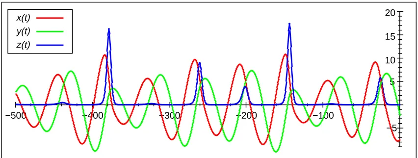
plotted in figure 3.1. x(t)andy(t)oscillate with a modulated amplitude. The phase difference
be-tweenx(t)andy(t)is almost constant.z(t)shows irregular peaks of varying size. The width and
height of the peaks is coupled to the modulation inx(t), which again is related toy(t). Therefore
the pattern of the peaks is very sensitive to initial conditions. The Roessler dynamics generates a chaotic trajectory in this sense.
A three dimensional view of the Roessler trajectory is depicted in figure 3.2. The flow consti-tutes basically a spiral in thexy-plane. This spiral is unwinding until the trajectory gets out of the xy-plane due to the peak in thez-coordinate. With the peak, it returns from its outer side to the
inner portion again. The connection of the outer with the central parts involves a twist that leads
−5 5 10 15 20
−500 −400 −300 −200 −100
x(t)
z(t) y(t)
24 3 The Training Setup
−10 0 10
−10 0 10 0 10 20
(a) View on thexz-plane.
−10 0 10
−10 0 10 0 10 20
(b) View on thexy-plane.
−10 0 10 −10 0 10 0 10 20
(c) View on theyz-plane.
Figure 3.2: 3d-view of the Roessler attractor.
to a formation similar to a Moebius band. Here, the flow is not confined to a surface but turns out to have two-dimensional cross sections that have the form of a horseshoe map. Hence it can be shown that the Roessler flow is non periodic and structurally stable. Its limit set is a strange attractor [see Rössler, 1976, and the references therein].
In summary, the Roessler equations (3.1) give rise to several interesting phenomena exhibited by nonlinear dynamical systems. An interesting question is whether the input-output operator implicitly given by the equations can be learned by a recurrent neural network and how different learning algorithms cope with the features of the Roessler flow. It is therefore tempting to use the Roessler attractor as a training task in the investigation of learning with recurrent neural networks.
3.2
The Network Architecture
The task of learning the operator implicit in the Roessler equations means that the network gets two coordinates as inputs and has to generate the third coordinate as output. This task was also used for a case study by Steil [1999]; Steil and Ritter [1999b]. It is known – and also intuitive – that the case of learningz(t)fromx(t)and y(t)is much harder than learningx(t)ory(t)from
the respective other two because the prediction of the width and the height of the peaks is difficult and strongly dependent on the time-course of the coordinates. Since the scope of this work was not to investigate what tasks can be learned but to compare the behavior of different algorithms, the easier task of learningy(t)fromx(t)andz(t)was used for the further analysis.
The network architecture was chosen to be a fully-connected recurrent neural network of ten neurons. The network has two inputsu
k
(t); k=1;2that are connected to every neuronx i
; 1
i10in the network with weightsw
ik. The activation of neuron x
iis given by the equation
_ x i = x i (t)+ 10 X j=1 w ij f(x j (t))+ 2 X k=1 w ik u k (t); (3.2)
wheref(x j
)=tanh(x j
). The output is taken from neuronx 1
o 1
(t)=x 1
(t): (3.3)
Equation (3.2) is rewritten in discrete form using Euler integration