Efficient Modular Arithmetic for SIMD Devices
Wilke Trei
Department of Mathematics, University of Oldenburg, 26111 Oldenburg, Germany, Phone: +494417983219
Abstract
This paper describes several new improvements of modular arithmetic and how to exploit them in order to gain more efficient implementations of commonly used algorithms, especially in cryptographic applications. We further present a new record for modular multiplications per second on a single desktop computer as well as a new record for the ECM factoring algorithm. This new results allow building personal computers which can handle more than 3 billion modular multiplications per second for a 192 bit module at moderate costs using modern graphic cards.
Keywords: Fast Modular Arithmetic, Improvements of Montgomery Reduction, Graphics Processing Unit, Factoring using Elliptic Curves
Introduction
Parallelization of computational intensive algorithms has always been an important task in computational number theory.
This task becomes even more crucial during the last years, since the clock rate of ordinary processors stagnates. Therefore the chip vendors begin to rise the numbers of computational units on a single chip in order to keep the performance increases high.
Simultaneously graphic cards – which classically have many computational units but lack of control flow units – got more and more programmable. With the introduction of NVidia’s CUDA technology and later the OpenCL platform, graphic cards came more and more into focus of programmers and security institutions, attracted by the high level of performance these chips may offer.
for efficient use of these chips, it is important to keep the chip’s internal parallelization high because these devices often adapts one single instruction to multiple data (SIMD). In this paper we present some algorithmic improvements to optimize modular arithmetic for this type of devices. This improvements are generic in the sense that they are neither specific for one special number theoretical algorithm, nor are they limited to SIMD use only.
In order to test our improvements in practice, we applied them to an highly efficient version of Lenstra’s ECM algorithm. Our implementation breaks the old record in terms of modular multiplication per second stated at Eurocrypt 2009 [1] and SHARKS 2009 [2].
We decided to use OpenCL for our implementation. Since OpenCL is a free standard and widely available, it is easy to keep compatibility with many soft- and hardware platforms. A detailed description of OpenCL can be found in Section 1. Descriptions of the ECM algorithm and our implementation are given in Section 3.
1. Heterogeneous Computing using OpenCL
1.1. Overview
OpenCL is an open programming model and standard for heterogeneous hardware plat-forms. Its first version was released in December 2008 by the Khronos Group [3] and is especially designed for parallel computations. The latest version of the standard was re-leased in November 2011 [4].
OpenCL is designed to offer a unified programming model for different hardware plat-forms. Like the NVidia CUDA platform OpenCL can for instance be used to program modern graphic cards. Furthermore it can be used to program ordinary x86 CPUs as well as IBM Cell Processors and several special purpose hardware. At the end of this section we give an overview on the commonly used OpenCL devices and its computational capabilities. We will describe the OpenCL programming platform briefly. An elaborate description can be found in [5].
The OpenCL platform model consists of two hardware components – a host and an
OpenCL device – that may or may not be the same. While the host must be a directly programmable device like a CPU, the OpenCl device must not have a stand-alone function-ality at all. An OpenCL device has its own memory location and offers several OpenCL Compute Units (CU). A compute unit can be an SIMD (single instruction multiple data) computational unit, thus compute units are the finest granularity for control flow in the OpenCL platform.
A compute unit is furthermore the location of so calledlocal memory that can be used to share data among threads quickly. Every compute units may hold arbitrarily many stream cores that are essentially arithmetical logical units (ALU). The stream core is the finest granularity for independent work threads, i.e. every stream core gets at least one ore more consecutive computational tasks.
applied to a single work item data. Kernels are usually executed in parallel on all available stream cores of an entire OpenCL device processing many work threads simultaneously.
The work items are normally grouped into so called work groups. A single work group is atomically executed on one compute unit and can use the local memory of this unit to share data among its work items. To share data with all other threads the devices memory, also called global memory, has to be used.
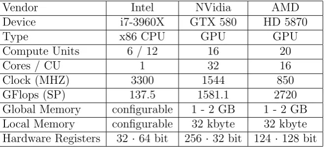
There are many different OpenCL devices on the market. The most commonly used are graphic cards. Table 1 gives a short overview of some common OpenCL devices and their computational capabilities.
Vendor Intel NVidia AMD
Device i7-3960X GTX 580 HD 5870
Type x86 CPU GPU GPU
Compute Units 6 / 12 16 20
Cores / CU 1 32 16
Clock (MHZ) 3300 1544 850
GFlops (SP) 137.5 1581.1 2720
Global Memory configurable 1 - 2 GB 1 - 2 GB
Local Memory configurable 32 kbyte 32 kbyte
Hardware Registers 32 · 64 bit 256 ·32 bit 124 · 128 bit
Table 1: On Market OpenCL Devices
1.2. Limitations
The most common OpenCL devices are so called SIMD devices, i.e. devices that have many computational cores working on data in parallel, but sharing the instructional data and the control flow. There are several bottlenecks on this type of devices, especially on graphic cards.
One major aspect are the so called race conditions. For example on a modern AMD graphic card at least 64 computational threads have to follow the same execution path in-dependent of their data. Thus in case of branches, that are not coherent among all glued units, every occurring path of the branch has to be calculated sequentially while those units not taking this path remain idle. [5, p. 135]
constant data is cached within the L2 cache. [6, appendix table D4]
There are two memory locations available for synchronizing work items. First of all there is the so called local memory that offers fast access and high throughput. This local memory is placed within the compute unit and has a size of roughly 16-32 kb depending on the OpenCl device used. The local memory is designed to share data among all work items that belong to the same work group, i.e. are running on the same compute unit.
The other memory usable for synchronization is the global memory and can be up to a few gigabytes in size. This memory offers much slower access than local or register space, but can share data among all work items. Furthermore this memory location is the place where initial data and result data is stored. One crucial task in programming with OpenCl is to control the use of the global memory carefully, because it is easily going to be the bottleneck in any parallelized algorithm.
Even when all this limitations are considered, the programming itself is not as simple as on ordinary processors due to more architectural differences. This affects especially programming AMD graphic cards prior to the HD7000 series. On this cards every compute core itself is a vector processor able to handle up to 4 or 5 low level operations in parallel. For example on a HD5800 type card one core can perform a single integer multiplication and up to 4 independent integer additions in parallel. The need of splinting a single task into vectorized operations is one of the main difficulties when dealing with these graphic cards. In order to make programming more similar to ordinary CPU programming or working with NVidia graphic cards, AMD changed the architecture from the HD7000 series onwards to compute a single operation per core per clock. [6, section 1.2]
2. Efficient Modular Arithmetic
2.1. Common Modular Arithmetic
For most computationally difficult number theoretic algorithms it is needed to chain a lot of modular operations with fixed module.
Currently there exist two important algorithms for modular reduction using the fact that the modulus is fixed in most cryptographic applications, namely the Barret and the Montgomery reduction algorithms.
Algorithm 1. Barret Reduction [7]
Let a, m∈N with a < m2 and m be an odd integer of binary length n =dlog
2 me.
Further-more, let R= 2n and µ=bR2
mc. The following algorithm computes a (mod m).
1. Calculate r=a−
ba Rc
µ R
m.
Algorithm 2. Montgomery Reduction [8]
Let a, m ∈ N with a < m2 and m be an odd integer of binary length n = dlog2 me. Furthermore, let R = 2n and m0 < R such that m·m0 ≡ −1 (mod R).
The following algorithm computes R−1·a (mod m).
1. Calculate b=a·m0 (mod R).
2. Calculate r= a+b·m
R over the integers.
3. If r≥m return r−m, else return r.
While the Barret Reduction gives the desired result immediately, the Montgomery Re-duction is usually used with a modified residue system modulom. In this case every element modulom is multiplied byR. Using this transformation the modular addition is untouched and the multiplication can be done by multiplying xR·yRover the integers and then exe-cuting the Montgomery Reduction giving xyR.
Both reduction themselves cost at most 2M(n) if we define M(n) to be the cost of a multiplication with input operands of size at mostn in terms of arithmetic operations. This claim holds, because the reduction modulo R and the division operations are only binary representation cutoffs, and since µ, R and m0 can be pre-calculated.
Although the Montgomery reduction consumes more addition operations than the Bar-ret reduction, we choose the latter algorithm for our implementation of modular reduction. This is especially due to the improvements provided in sections 2.2 and 2.3. For the rest of this paper we assume the size of the modulusm is given byn =dlog2 me.
We recall that the cost of a modular multiplication is bounded by the cost of an ordinary multiplication of integers. Thus, it is crucial to know the integer multiplication methods when dealing with modular multiplication.
The classical schoolbook multiplication splits the input operands a, b of size n into two partsa =a1·2d
n
2e+a0, b =b1·2d
n
2e+b0 where a1, a0, b1, b0 are integers of size at mostdn
2e. Then it performs the entire multiplication by calculating four products of half-size integers
ab=a1b122d
n
2e+ (a1b0 +a0b1)2d
n
2e+a0b0.
This operation is used recursively until the machine word size is reached, i.e. the multipli-cations can be performed by the machine directly. The cost of this method is asymptotically O(n2).
complexity class ofO(n) can be obtained with arbitrarily close to 1 for increasing k. The
algorithm makes use of the evaluation homomorphism and the possibility to interpolate a polynomial of degreek when k+ 1 points on its graph are known.
Algorithm 3. Toom-Cook-k [10]
Let a, b be integers of length n and k a fixed positive integer. Assume the binary represen-tation of a and b is split into k parts
a=
k−1
X
i=0
ai 2i·d
n ke
b=
k−1
X
i=0
bi 2i·d
n ke.
Then define the polynomials
¯
a:=
k−1
X
i=0
ai xi ∈Z[x]
¯
b :=
k−1
X
i=0
bi xi ∈Z[x].
Obviously a = ¯a(2dnke) and b = ¯b(2d n
ke) and due to the evaluation homomorphism ab =
(¯a·¯b)(2dnke). Since the product polynomial of ¯a and¯b has degree 2k−2, this product can be calculated as follows.
1. Select 2k −1 small distinct integers x0, . . . , x2k−2 and calculate the evaluations yi =
¯
a(xi) and zi = ¯b(xi).
2. For all 0≤i <2k−1, calculate the products wi =yizi.
3. If the evaluation points xi are selected carefully, one can interpolate ¯a ·¯b from the
known points wi = (¯a·¯b)(xi) using linear algebra.
4. Evaluate ¯a·¯b at 2dnke to obtain the integer product of a and b.
Remark 1. Usually the first one of the evaluation points in Algorithm 3 is chosen to be 0, so w0 is essentially a0b0. Furthermore one often assumes that the polynomials are evaluated
at x2k−2 =∞, i.e. their highest coefficients are multiplied.
Using this notation the Toom-Cook-2 algorithm with evaluation at0,1 and ∞ is exactly the Karatsuba-Ofman algorithm.
Algorithm 3 dividesa and b intok parts and needs 2k−1 multiplications beside several bit-shifts, multiplication with small constants etc. Thus the algorithm has an asymptotically complexity ofO(nlogk2k−1) and hence for every >1, a complexity ofO(n) can be achieved
Due to the overhead in steps 1,3 and 4 the Toom-Cook algorithms are only practical in a certain range. Usually after the inputs became 10-100 times the machine word size the arith-metic switches from schoolbook multiplication to the Karatsuba-Ofman algorithm. Later Toom-Cook-3 and Toom-Cook-4 become faster. Finally the Sch¨onhage-Strassen algorithm [11] – that has currently fastest asymptotically complexity of an multiplication algorithm, i.eO(nlognlog logn) – is more often used than Toom-Cook-k for k exeeding 5.
2.2. Avoidance of Reduction Operations
As mentioned in the restrictions section it is necessary to avoid as many branches as possible and to keep the existing ones short. For modular arithmetic there is at least one barely avoidable branch dealing with reduction operations after over- or underflows.
On a SIMD device the branch times adds up, thus it does not matter if a reduction operation is performed every times when possible. The correct result simply can be selected afterwards. Therefore it is a common optimization to substitute the decision and reduction operations after additions or subtractions by the following algorithms.
Algorithm 4. Reduction after Addition
Let a be an integer with 0≤a <2m. Then the reduction of a (mod m)can be computed by
1. Calculate a0 =a−m.
2. If a0 <0 return a, else return a0.
Algorithm 5. Reduction after Subtraction
Let a be an integer with −m ≤ a < m. Then the reduction of a (mod m) can be computed by
1. Calculate a0 =a+m.
2. If a <0 return a, else return a0.
These algorithms have the advantage of very simple decisions depending only on a single bit. Furthermore they are simple to implement using OpenCl, since OpenCl offers very efficient selection operations and thus they cause only very short branches.
For our implementation we also use an observation on the Montgomery reduction that helps avoiding reduction operations after every multiplication step.
Lemma 1. Reduction Capabilities of the Montgomery Reduction
Letm ∈Nbe an odd integer of binary length n=dlog2 meand R, R0 being powers of2with R≥4R0 = 2n. Then the following observations can be made for the Montgomery Reduction algorithm (redc) applied to R and m.
1. Let a, b be integers with a, b <2R0. Then redc(a·b)≤R0 +m <2R0.
Proof. The product ofa andb is less or equal to 4R02 which is bounded byRR0. Due to the function principle of the REDC algorithm this implies that
redc(a, b) = mN +ab
R <
RN +RR0
R =R
0
+N.
The second claim can be proven analogously.
The Lemma allows to build multiplication chains without any intermediate reduction. In order to use this improvement, we ensure in our implementation, that our total work width is at least two bit wider than our modulus. That is why our OpenCL implementation of the ECM algorithm is currently limited to use integers up to 2254 instead of 2256. Furthermore we decided to allow representatives between 0 and 2log2m+1−1 instead of 0 andm wherem
is our modulus. Hence it may be required to add 2minstead of mafter a subtraction. Since after nearly every subtraction a multiplication follows, it causes no disadvantage to add the precomputed 2m.
In this fashion we are able to limit the Reduction after Addition/Subtraction operations from total 19 to 11 executions within our algorithms main loop.
2.3. Faster Truncated Multiplication
One key task of both reduction algorithms described in Section 2.1 is to use truncated multiplications, i.e. to perform multiplications where only one half of the results binary representation is needed for further use. In order to make the reduction operations as cheap as possible, it is a natural attempt to use the fact that one half of the product may be easier to calculate. For the lower half multiplication result there are well known methods to compute it in less time than the time for the full product.
Algorithm 6.
Let a, b be integers of length n and let ρ be a parameter in the interval [0.5,1]. Then one can calculate a·b (mod 2n) the following way.
1. If a=
n−1
P
i=0
ai2i and b = n−1
P
i=0
bi2i calculate P0 =
dρ(n−1)e
P
i=0
ai2i ·
dρ(n−1)e
P
i=0
bi2i.
2. Calculate the lower halves of the products P1, P2 satisfying
P1 =
n−1
X
i=dρ(n−1)e ai2i·
n−1−dρ(n−1)e
X
i=0
bi2i
P2 =
n−1−dρ(n−1)e
X
i=0
ai2i· n−1
X
i=dρ(n−1)e bi2i.
The case ρ = 1 in Algorithm 6 is exactly the case where the full product is calculated during step 1 and afterwards is reduced mod 2n. The caseρ= 0.5 is the average case when dealing with the classical schoolbook multiplication. In this case P0 is equal to a0b0 and
P1 respectively P2 are the products a1b0 and a0b1. The optimal choice of ρ depends on the efficiency of the underlying multiplication algorithm.
Theorem 2. Optimal ρ for Algorithm 6 [12, Section 2]
Given a multiplication algorithm with complexity O(nα), α∈]1,2]. Then the runtime S(n)
of Algorithm 6 is at most
S(n) = M(ρn) + 2S((1−ρ)n)≤CρM(n), with
Cρ=
ρα
1−2(1−ρ)α.
The minimum value of Cρ is reached at
ˆ
ρ= 1−2α−−11.
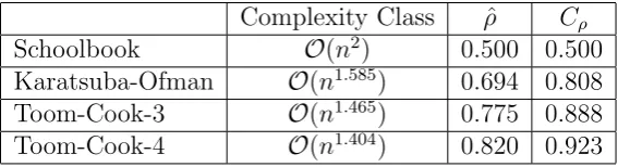
It is easy to see that for decreasing α the quantity Cρ of Algorithm 6 is tending to one.
Thus a more efficient multiplication algorithm is less advantageous to calculating only half products. Table 2 gives some values for ˆρandCρin the case of the multiplication algorithms
discussed in Section 2.1.
Complexity Class ρˆ Cρ
Schoolbook O(n2) 0.500 0.500
Karatsuba-Ofman O(n1.585) 0.694 0.808
Toom-Cook-3 O(n1.465) 0.775 0.888
Toom-Cook-4 O(n1.404) 0.820 0.923
Table 2: ˆρandCρ for several multiplication algorithms
Due to the missing carry bits from the lower half product, a method similar to Algorithm 6 is hard to achieve for the more significant bits of a multiplication. First attempts where to calculate some additionalguard bits to correct the error of missing carry bits [13].
For our purpose we found an astonishingly simple to use way to save operations in the calculation of the high half truncated product in step 2 of the Montgomery Reduction algo-rithm.
In the setting of the Montgomery multiplication it is necessary to calculate the most significant bits of the integer a +b · m. By proving the correctness of the Montgomery reduction algorithm one already knows that b·m ≡ −a (mod R) for any input number a. This fact can be used to save operations during the calculation of b·m, since the lower half of its binary representation is already known.
We will demonstrate this advantage in the case of the schoolbook multiplication.
Theorem 3.
Let n, M(n)be defined as before. Then the Montgomery Reduction algorithm for a modulus m of size n can be computed in 1.25M(n) plus a few addition operations without the need of wooping or guard bits.
Proof. Let the lower half product b = am0 (mod R) already be calculated and let m =
m12d
n
2e+m0 and b=b12d
n
2e+b0 be the split binary representations of mand b respectively.
Then we know that
b·m =m1b122d
n
2e+ (m1b0+m0b1)2d
n
2e+m0b0 ≡ −a (mod R)
from the definition of the schoolbook multiplication and our observation. We assume
R = 22dn
2e holds since n is often ceiled to the next multiple of the machine word size, thus
we can calculate
m0b0 ≡ −(a+ (m1b0+m0b1)2d
n
2e) (mod R)
instead of multiplying m0b0 directly. This way one saves one of the four multiplications giving 0.5M(n) + 0.75M(n) as approximate total runtime.
This method is theoretically slower than wooping-based attempts for schoolbook mul-tiplications. Since there is no need for an error correction it may be more practicable for small operand sizes. For growing n one can even outperform whooping based attempts.
Theorem 4. Let the notation from Algorithms 2 and 3 be given. Then one easily can calculate the full product in step 2 of Algorithm 2 using 2k −2 instead of 2k − 1 sub-multiplications.
Proof. The idea is to avoid the calculation of the lowest significant bits in the binary repre-sentation of b·m. In detail the calculation of ¯b(0) ¯m(0) can be replaced using the following algorithm.
1. Assume x0 = 0 and wi = ¯b(xi) ¯m(xi) were calculated for all i > 0 using 2k −2
2. Compute w0,L = −a (mod 2d
n
2e). Since w0 = ¯b(0) ¯m(0) is an integer less than 22d
n
2e,
w0,L is exactly the lower half of the binary representation of w0.
3. Use w1, . . . , w2k−2, w0,L in order to compute the lower order digitsl0 of the linear term of the polynomial b·m. This works because the full linear term can be obtained from the full representations ofw0, . . . , w2k−2.
4. Now one can recover the full product ¯b(0) ¯m(0) =−a−l02d
n
2e (mod 22d
n
2e).
Table 2 shows the theoretical relative runtime ˆCM(n) of the methods described in The-orems 3 and 4 compared to the classical approach combined withguard bits or wooping.
Cρ Cˆ
Schoolbook 0.500 0.750
Karatsuba-Ofman 0.808 0.667
Toom-Cook-3 0.888 0.800
Toom-Cook-4 0.923 0.857
Table 3: Wooping compared to theorems 3 and 4
Note that this optimizations makes the computation of our higher half truncated products faster than for the lower half ones. Furthermore from Toom-3 onwards there are more unused bits that may be used for further optimizations. This is one of the subjects of future work on this topic.
3. ECM on Graphic Cards
For the evaluation of our arithmetical ideas we choose the ECM algorithm as a testing application. The ECM algorithm was first described by H.W. Lenstra Jr. in 1987 [15] and was later improved by P. L. Montgomery [16] and many others. A single staged version of the algorithm is stated below.
Algorithm 7. Elliptic Curve Method, Stage 1 [15]
Let n be a composite integer and B1 a suitable bound. The following probabilistic algorithm
can be used to find a factor of n.
1. Calculate the constant k = Q
p∈P,p≤B1
pep with pep ≤B
1 < eep+1, ep ∈N.
2. Pick a random elliptic curve E over Z/nZ and a point O 6=P ∈EZ/nZ.
3. CalculatekP onEZ/nZ. If this fails one denominator within the group law formulas is
There are several ways to implement this algorithm. One important choice is the model of the used curves. A common way is to use projective curves in Montgomery coordinates [17] or Edwards coordinates [18].
Although elliptic curves in Edwards coordinates may have a slightly more efficient group law we decided to use Montgomery curves for our first prototype in order to keep compat-ibility with common implementations, especially the Brent-Suyama parametrization [19]. Previous implementations of the ECM algorithm on graphic cards by Bernstein et al. used floating point arithmetic [1] or 24 bit multiplication [2] for building their long integer arith-metic. Although even for our used AMD HD 5000 series graphic cards the 24 bit performance is roughly 5 times higher than for the ordinary 32 bit multiplication, we decided to use the latter to build up our arithmetic. This is done because in contrast to the 24 bit case OpenCL offers an easy to use command to get the higher order bits of an 32 bit multiplication. Fur-thermore during a 32 bit multiplication several additions can be performed in parallel, hence our code is designed to process carry bit calculations of previous multiplications in parallel to our current ones.
The parallelization is straight forward. Every work-item is assigned to a single elliptic curve plus a starting point and has to process the scalar multiplication of the point described in step three of algorithm 7. Since we build our program to handle 254 bit integers – 8·32 minus the two bits described in section 2.2 – and every item has to store the curve param-eters, three copies of point coordinates and some temporary space, we are using roughly half of the 124 registers available. Thus if one is careful with scratch space even 510 bit arithmetic should work the same way. Building wider arithmetic is one of the subjects for further improvements of our implementation.
An important fact of this simple parallelization is the absence of need for synchronization between two threads. Even if not crucial, this helps a lot exploiting the maximum modular multiplication per second capabilities of modern graphic cards. Beside the arithmetic de-scribed in Section 2 we use a carry select circuit on the low level.
An early version of the program lacking the improvements in Sections 2.2 and 2.3 and several other improvements won a prize for innovative use of OpenCl assigned by AMD and TopCoder [20].
4. Experimental Results
APP SDK 2.5 on Ubuntu 11.10 x64 as our software platform.
All tests have been done on a 254 bit module and B1 fixed to 8192. For a better comparison to previous attempts to implement the ECM algorithm we scaled the results by (254192)2. Table 4 shows this scaled results as well as the prize / performance ratio for our implementations. In order to compare the prize / performance ratio it is necessary to know that the previous records were achieved by using a 500$ NVidia Geforce GTX295 graphics card while our HD5870 has an average market prize of 320$ as of January 2012.
MulMod·106 / Sec MulMod·106 / (Sec · $)
Previous Record [2] 575 1.15
AMD Challenge Version [20] 430.8 1.34
Recent Optimized Version 846.2 2.64
Table 4: 192 bit MulMod / sec in our implementations
Note that our implementation currently is able to handle 3756 scalar multiplications per second on an elliptic curve over a 254 bit modulus. Scaled to 192 bit these are roughly 6575 curves per second. Although this also is a new record for ECM on a single-chip graphics card it is not as much as it may be. The program of Bernstein et. al. [2] is capable of processing 4928 scalar multiplications per second by much less modular multiplications. We believe this gap occurs since we do not multiply out our module and do not use the arithmetical advantages of Edwards curves yet.
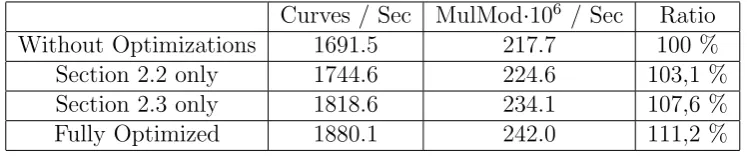
In order to evaluate the impact of our observations described in Sections 2.2 and 2.3 we ran about 51.200 scalar multiplications with B1 = 8192 and on a 254 bit modulus with OpenCL kernels without these improvements. Note that we used an AMD Radeon HD 5770 graphic card for our experiments that has exactly half the computational capabilities of the earlier described HD 5870 model.
Curves / Sec MulMod·106 / Sec Ratio
Without Optimizations 1691.5 217.7 100 %
Section 2.2 only 1744.6 224.6 103,1 %
Section 2.3 only 1818.6 234.1 107,6 %
Fully Optimized 1880.1 242.0 111,2 %
Table 5: 254 bit MulMod / sec for different optimization stages on HD 5770
We see that our observations can deliver up to 11% more arithmetical throughput for free, while being easy to implement.
700$ for the two graphic cards and additionally a few hundred $ for the peripheral compo-nents. In total a total cost of 2000$ should not be exceed.
This level of computational throughput is already in the range of being relevant for modern security. For example the elliptic curve discrete logarithm problem with a 130 bit module – as used in one of the Certicom ECC challenges – was believed to be infeasible for long. Using our 400 of our described 3 billion modular multiplication per second computers, this challenge is theoretically in range to be broken within a year under common runtime assumptions [21].
Summarizing SIMD devices offer a lot of computational potential and significance whereas there is still room left for more technical and algorithmical improvements.
References
[1] D. J. Bernstein, T.-R. Chen, C.-M. Cheng, T. Lange, B.-Y. Yang, ECM on Graphics Cards, Cryptology ePrint Archive, Report 2008/480 (2008).
[2] H.-C. C. M.-S. C. C.-M. C. C.-H. H. T. L. Z.-C. L. B.-Y. Y. Daniel J. Bernstein, The billion-mulmod-per-second PC, Workshop record of SHARCS’09: Special-purpose Hardware for Attacking Cryptographic Systems (2009).
[3] K. Group, The Khronos Group Releases OpenCL 1.0 Specification,
http://www.khronos.org/news/press/the khronos group releases opencl 1.0 specification (2008). [4] K. Group, Khronos Releases OpenCL 1.2 Specification,
http://www.khronos.org/news/press/khronos-releases-opencl-1.2-specification (2008).
[5] B. Gaster, D. Kaeli, L. Howes, P. Mistry, Heterogeneous Computing with OpenCL, Morgan Kaufmann Pub, 2011.
[6] A. M. Devices, AMD Accelerated Parallel Processing Programming Guide, v1.3f, http://developer.amd.com/sdks/AMDAPPSDK/assets/AMD Accelerated Parallel
Process-ing OpenCL ProgrammProcess-ing Guide.pdf (2011).
[7] P. Barrett, Implementing the Rivest Shamir and Adleman public key encryption algorithm on a stan-dard digital signal processor, in: Advances in CryptologyˆaCRYPTOˆa86, Springer, 1987, pp. 311–323. [8] P. Montgomery, Modular multiplication without trial division, Mathematics of computation 44 (170)
(1985) 519–521.
[9] A. Karatsuba, Y. Ofman, Multiplication of multidigit numbers on automata, in: Soviet physics doklady, Vol. 7, 1963, p. 595.
[10] S. Cook, On the minimum computation time for multiplication, Doctoral diss., Harvard U., Cambridge, Mass.
[11] A. Sch¨onhage, Asymptotically fast algorithms for the numerical muitiplication and division of polyno-mials with complex coefficients, Computer Algebra (1982) 3–15.
[12] T. Mulders, On Computing Short Products, Tech. rep. (1997).
[13] L. Hars, Fast truncated multiplication for cryptographic applications, Cryptographic Hardware and Embedded Systems–CHES 2005 (2005) 211–225.
[14] K. Bentahar, N. Smart, Efficient 15,360-bit RSA using woop-optimised montgomery arithmetic, Cryp-tography and Coding (2007) 346–363.
[15] H. W. Lenstra Jr., Factoring with Elliptic Curves, Annals of Mathematics 126 (1987) 649–673. [16] P. Montgomery, An FFT extension of the elliptic curve method of factorization, Ph.D. thesis,
UNI-VERSITY OF CALIFORNIA Los Angeles (1992).
[18] D. J. Bernstein, P. Birkner, T. Lange, C. Peters, ECM using Edwards curves, IACR Cryptology ePrint Archive 2008 (2008) 16.
URLhttp://eprint.iacr.org/2008/016
[19] P. Zimmermann, B. Dodson, 20 years of ECM., Hess, Florian (ed.) et al., Algorithmic number theory. 7th international symposium, ANTS-VII, Berlin, Germany, July 23–28, 2006. Proceedings. Berlin: Springer. Lecture Notes in Computer Science 4076, 525-542 (2006). (2006). doi:10.1007/11792086. [20] A. M. Devices, AMD OpenCL Coding Competition, http://community.topcoder.com/amdapp/ (2011). [21] A. K. Lenstra, E. R. Verheul, Selecting Cryptographic Key Sizes., in: H. Imai, Y. Zheng (Eds.), Public