Comparative Study of Subspace Clustering
Algorithms
S.Chitra Nayagam,
Asst Prof., Dept of Computer Applications, Don Bosco College, Panjim, Goa.
Abstract-A cluster is a collection of data objects that are similar to one another within the same cluster and are dissimilar to the objects in other clusters. Subspace clustering is an enhanced form of the traditional clustering which is used for identifying clusters in high dimensional data sets. There are two major subspace clustering approaches namely : Top-down approach which use sampling techniques that randomly pick up sample data points to identify the subspace and then assigns all the data points to form original clusters and Bottom-up approach, where dense regions in low dimensional spaces are found and then combined to form clusters.
The paper discusses details of the top-down algorithm PROCLUS which is applied for customer segmentation, Trend Analysis, Classification, etc. which needs disjoint partition of datasets and CLIQUE which is used to identify overlapping clusters. The paper highlights the important steps of both the algorithms with flowcharts and an experimental study has been carried out using synthetic data to compare PROCLUS and CLIQUE by varying dimensions of the data set, the size of the data set and the number of clusters.
Keywords : PROCLUS, CLIQUE, subspace, k-medoid, density threshold
1 INTRODUCTION
The process of grouping a set of physical or abstract objects into classes of similar objects is called clustering. The similarities between the objects are often determined by the distance measures over the dimensions of the data set. There are various challenging requirements of the clustering algorithms. This includes the insensitivity towards the order of inputs during cluster formation, scalability towards large data sets, finding overlapping clusters, finding clusters of arbitrary shape, finding outliers or noisy data. The major drawback of the traditional clustering algorithms to meet all these challenges is its inability to handle high dimensional data set which is considered to be the “curse of dimensionality” where the performance degrades as the dimensions increases.
Subspace clustering algorithms came into existence to solve these problems. A subset of dimensions from the high dimensional data set used to identify clusters is called “subspace clustering”. There are two different approaches for finding subspace clustering: top-down approach and bottom-up approach.
1.1 Contributions
This paper considers the subspace clustering algorithms PROCLUS from top-down and CLIQUE from bottom-up approaches and had performed a comparative study between the top-down and bottom-up approaches of the subspace clustering algorithms.
A performance study has been carried out during our experimentation in order to find the scalability and efficiency of the two algorithms. The contributions to this paper were also focused towards the algorithms PROCLUS
and CLIQUE by making them simple to understand using
flow charts.
1.2 Organization of the paper
In section 2, CLIQUE algorithm has been discussed with flow chart. In section 3, PROCLUS algorithm has been discussed with flow chart. The performance analysis of both the algorithms have been discussed in section 4 and section 5 contains the conclusion.
2 BOTTOM-UP APPROACH
The algorithms in this approach creates histogram bins for each dimension and selecting only those bins which have densities above the given threshold value. This approach uses the downward closure property of density to reduce the search space by using an APRIORI style approach. This downward closure property of density means that if a collection of points S is a cluster in a k-dimensional space, then S is also part of a cluster in any k-1 dimensional projections of this space. Candidate subspaces for the next higher level of dimension sets are formed only from the lower level meaningful dimensions that have formed the dense regions. The algorithm stops only where there are no more dense regions. Adjacent dense units are then combined to form clusters. Most of the bottom-up algorithms find overlapping clusters by assigning a data point to more than one cluster. CLIQUE is one among the first such algorithm.
2.1 CLIQUE algorithm
CLIQUE is the short term for CLustering In QUEst developed by R.Aggrawal[3] which is a top-down approach based subspace clustering algorithm that starts by placing each object in its own cluster and then merges the atomic clusters into larger and larger clusters until all objects are placed in a larger cluster. CLIQUE automatically identifies subspaces with high-density clusters. It produces identical results irrespective of the order in which the input records are presented without presuming any canonical distribution for input data.
The Problem: Given a set of data points and the input parameters, ξ and τ, find clusters in all subspaces of the original data space and present a minimal description of each cluster in the form of DNF expression. The algorithm consists of three phases.
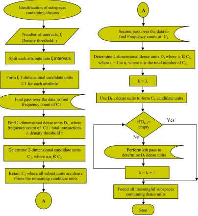
2.1.1 Identification of subspaces that contain clusters
clustering criterion with respect to dimensionality to prune the search space.
The algorithm proceeds level-by-level. It first determines 1-dimensional dense units by making a pass over the data. Then it uses these dense units to form the 2-dimensional dense units by making another pass over the data. Having determined (1) dimensional dense units, the candidate k-dimensional units are determined using the candidate generation procedure. The candidate generation procedure takes as an argument Dk-1, the set of all (k-1) dimensional
dense units. It returns a superset of the set of all k-dimensional dense units. A pass over the database is made
to find those candidate units that are dense. The algorithm terminates when no more candidate units are generated. Dk-1 dense units have to be self-joined, where the units
share the first k-2 dimensions. The algorithm discards those dense units from Ck which have a projection in (k-1)
dimensions that is not included in Ck – 1. As the
dimensionality of the subspaces increases, the dense units start exploding which leads to the need of pruning the candidates. The pruned dense units are then used to form the next level candidate units which generate the next level dense units.
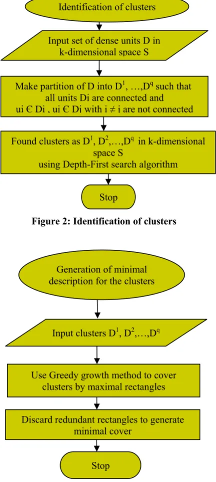
2.1.2 Identification of clusters
The input for this phase is a set of dense units D, all in the same k-dimensional space S. The output will be a partition of D into D1, …,Dq, such that all units Di are connected and
no two units ui Є Di , ujЄ Dj with i ≠ j are connected. Each
such partition is a cluster formed by using depth-first search (DFS) algorithm to find the connected component in the graph formed by representing the dense units as the vertices of the graph. An edge exists between those vertices whose corresponding dense units have a common face.
Figure 1: Identification of subspaces containing clusters Identification of subspaces
containing clusters
Split each attribute into ξ intervals
Form ξ 1-dimensional candidate units C1 for each attribute
First pass over the data to find frequency count of C1
Find 1-dimensional dense units D1, where
frequency count of C1 / total transactions
≥ density threshold τ
Determine 2-dimensional candidate units C2, where uiujЄ C2
Retain C2 where all subset units are dense
Prune the remaining candidate units
A Number of intervals, ξ
Density threshold, τ
Second pass over the data to find Frequency count of C2
A
Determine 2-dimensional dense units D2 where uiЄ C2,
where i = 1 to n, where n is the total number of C2
k = 3,
Use Dk-1 dense units to form Ck candidate units
if Dk-1=
empty
Perform kth pass to determine Dkdense units
Found all meaningful subspaces containing dense units
Stop k = k + 1
Yes
2.1.3 Generation of minimal cluster description
This phase takes the clusters formed from second phase and generates a concise description for it. For this purpose, it uses a greedy growth method to cover clusters by a number of maximal rectangles (regions), and then discards the redundant rectangles to generate a minimal cover.
Figure 2: Identification of clusters
Figure 3: Generation of minimal cluster description
3. TOP-DOWN APPROACH
It starts by finding an initial approximation of the clusters in the full data space. Here, each dimension is assigned a weight for each cluster. The updated weights are used in the next iteration to regenerate clusters. The number of iterations varies in each algorithm based on the objective function used. Mostly, top-down approach algorithms use sampling technique to identify the cluster centers by
detecting the final correlated dimension sets for each cluster. These algorithms are mostly used to form clusters with disjoint partition sets where each instance of a data set belong to only one cluster. The input parameter plays a vital role in the quality of the clusters.
3.1 PROCLUS algorithm
A Projected cluster is formed with a subset of data points C and a subset of dimensions D where the points in C are closely related in the subspace dimension set D.
The PROCLUS algorithm uses a top-down approach which creates clusters that are partitions of the data sets, where each data point is assigned to only one cluster which is highly suitable for customer segmentation and trend analysis where a partition of points is required. The algorithm is capable of finding outlier set also.
PROCLUS [1] uses sampling technique to select sample data set and sample medoid set. K-medoids method is used in this algorithm to obtain cluster centres which determines the original clusters. The algorithm uses a three phase approach consisting of initialization, iteration and cluster refinement. The inputs for the algorithm are the number of clusters k, the average dimensionality l, and the two constants A,B which are apart from the input data set .
3.1.1 Initialization phase
The algorithm uses the greedy technique to find a good superset of piercing set of medoids. In order to find k clusters from the data set, the algorithm picks a set of points which are few times larger than k. This phase includes two steps to choose the superset. In the first step, it chooses a random sample data points whose size is proportional to the number of clusters that the user wish to generate which is given as,
S = random sample size A.k, where A is a constant and k represents the number of clusters.
The second step which uses the greedy method is performed to obtain a final set of points B.k, where B is small constant. This set is denoted as M where hill climbing technique is applied during the next phase.
3.1.2 Iterative phase
The iterative phase starts by randomly choosing a set of k -medoids, namely Mcurrent from the medoid set M found in initialization phase. The algorithm proceeds further by improving the cluster quality by iteratively replacing the bad medoids in the current set with the new medoids from M. The newly formed meaningful medoid set is denoted as Mbest. The algorithm uses a best objective function to determine the final medoid set Mbest. The algorithm begins by assigning an infinity value to BestObjective function and then randomly selects k medoids from the medoid set M which forms the set Mcurrent. The iteration begins then.
For each medoid mi in M, determine the minimum
manhattan segmental distance from other medoid to mi and assign as δi. Then, determine Li, which defines the locality to be the set of points that are within the radius δi from mi. The current objective function is checked against the BestObjective function and if the objective function obtained is lower than the BestObjective then the newly found value replaces the BestObjective. The next step is to determine the bad medoids and to replace them with the new one. The medoid of any cluster with less than (N / k) . Make partition of D into D1, …,Dq such that
all units Di are connected and ui Є Di , uj Є Dj with i ≠ j are not connected
Found clusters as D1, D2,…,Dq in k-dimensional
space S
using Depth-First search algorithm
Stop
Input set of dense units D in k-dimensional space S Identification of clusters
Input clusters D1, D2,…,Dq
Use Greedy growth method to cover clusters by maximal rectangles
Discard redundant rectangles to generate minimal cover
Stop
minDeviation points is assumed to be a bad medoid or outlier, where minDeviation is a constant smaller than 1 and is chosen in the algorithm to be 0.1.
This iterative phase continues till there is no change in the objective function for some ‘n’ number of times and then it terminates.
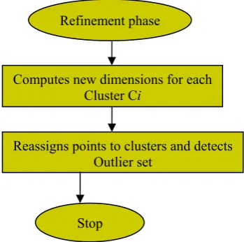
3.1.3 Refinement phase
The final step of this algorithm is refinement phase. This phase is included to improve the quality of the clusters formed. The clusters C1,C2,C3,…,Ck formed during the iterative phase are the inputs to this phase. The original data set is passed over one or more times to improve the quality of the clusters. The dimension sets Di found during the iterative phase are discarded and new dimension sets are computed for each of the cluster set Ci. Once when the new dimensions are computed for the clusters, then the points are reassigned to the medoids relative to these new sets of dimensions. Outliers are determined in the last pass over the data.
Figure 4: Flow chart of Initialization phase
Figure 5: Flow chart of Iterative phase
Figure 6: Flow chart of refinement phase
4 PERFORMANCE STUDY
An experimental performance study of all the three subspace clustering algorithms such as CLIQUE, PROCLUS and FINDIT has been carried out using synthetic data sets. The objective of the experiments undergone is to compare the performance of the two algorithms with respect to accuracy and time efficiency. The comparisons were performed by varying the data set size, varying the dimension size of the data set and varying the dimensions of the clusters. The experiments were conducted on Intel® Core™ 2 Duo CPU, E800 @ 2.66 GHZ. with 1.98GB RAM machine.
The synthetic data generation method described in [3] has been used for the data generation. The implementation for all the three algorithms has been carried out during this research.
4.1 Varying data size, by keeping dimensions of the data space fixed: For the first set of experiment, we have kept the dimensions of the data space to be fixed as 50 and Computes new dimensions for each
Cluster Ci
Reassigns points to clusters and detects Outlier set
Refinement phase
S = random sample of data points
Selects B.k number of medoids from the sample set S > k
using greedy technique based on manhattan segmental distance and name it set M ( ∑ i∊D | x1i - x2i | ) / D
Stop Initialization Phase
Chose random set k medoids, Mcurrent
For each medoid, assign points as Li centered within radius δi
Find dimension sets for each medoid
whose statistical average distance is smaller, total dimension = k * l
Find clusters - Manhattan segmental
distance is used to assign points for each k using selected dimension sets of each medoid
A
Find objective function to evaluate clusters
Replace bad medoid with new medoid – continue iteration until termination criterion (untilno
change in the process for some’n’ times)
Stop Iterative Phase
we have varied the number of records from 50,000 to 2,00,000. The total number of input cluster was kept as one with five dimensions. Figure 7 shows the results of the experiments conducted on PROCLUS and CLIQUE. Keeping fixed dimension and varying data sets – Forming One cluster
Figure 7: Scalability with number of records
4.2 Varying dimensions of the data space, by keeping the data set size fixed
In the second set of experimentation, the data set size has been fixed to 100,000 points and the dimensions had been changed as 25, 50, 75 and 100. This time the cluster dimensions have been increased. The data set had two input clusters: one with five dimensions and the other with seven dimensions. The two algorithms were executed for the experimentation and the execution time was computed. Figure 8 shows the result of CLIQUE and PROCLUS subspace clustering algorithms.
Keeping fixed data set size and varying dimensions - Forming TWO clusters
Figure 8: Scalability with the dimension of the data space
4.3 Interpretation of the results
PROCLUS shows good results with respect to the accuracy of the clusters formed. The execution time linearly increases with increase in dimension set for both the algorithms. This is due to the fact that a single pass over the database is required to assign the data points for each of the iteration while computing the bad medoids to replace with another medoid. CLIQUE discovers only one cluster with five dimensions in all cases of our experimentation and
fails to discover the cluster with seven dimensions when the input density threshold was set to 0.2.
When we decrease the density threshold to discover all the clusters, the algorithm has shown a very poor performance in execution time for all the cases. We tried to detect the missing cluster by reducing the density threshold factor τ to be 0.08 but it failed to detect the high dimensional cluster. When we still tried to decrease the value of τ to 0.04, the execution time of the algorithm rapidly increases because more time was spent in detecting the dense units.
The poor performance result is due to the fact that, as the volume of the cluster increases, the cluster density decreases [3]. CLIQUE’s output quality and execution time performance highly depends on tuning the input parameters
τ and ξ.
5 . CONCLUSION
We have compared the various strengths and weaknesses of the two approaches of subspace clustering by implementing and analyzing the algorithms- CLIQUE from bottom-up and PROCLUS from top-down. The synthetic data sets had been generated for our experimentation. The various features and requirements of these algorithms are summarized and shown in Figure 9.
Requirements /
Features CLIQUE PROCLUS
Efficiency
O(Ck + mk)
C – constant m – number of input points
k – highest dimensionality of any dense unit
O(N.k.d) N – number of Records k – number of clusters d – number of dimensions of the data set
Input threshold τξ – dense units – intervals for candidate units
k – number of clusters l – average dimensionality Domain
Knowledge of cluster formation
NO YES
Nature of cluster Overlapping Disjoint User specific
iterative threshold
NO, iterations stops when no more dense units are formed
YES, termination criteria Cluster quality misses high dimensional clusters and performs excellent with low dimensional clusters
detects all high dimensional clusters
Outlier set detection
misinterpretation of cluster points as outliers
Good performance in detecting Figure 9: Findings of algorithms
In this paper, we have reported the experimental results of the PROCLUS and CLIQUE algorithms as a performance study in a comparative manner. The choice of an algorithm depends purely on the application. For applications like trend analysis where disjoint partitions of data set is required, PROCLUS is suitable, and in the applications of overlapping cluster formation, CLIQUE is suitable.
0 50 100 150 50, 000 1,0 0,0 00 1,5 0,0 00 2,0 0,0 00 PROCLUS 10 50 80 150 CLIQUE 2 3 5 7
Runni ng t ime in sec. PROCLUS CLIQUE 0 20 40 60 80
25 50 75 100
PROCLUS 56 60 61 65
CLIQUE * 3 5 6 7
Runni ng t im e i n Sec. PROCLUS CLIQUE *
CLIQUE*
identifies only low dimensional clus
REFERENCES
[1] C.C. Aggarwal, J.L. Wolf, P.S. Yu, C. Procopiuc, J.S. Park, Fast algorithms for Projected clustering, in proceedings of the ACM SIGMOD international conference on management of data, ACM Press, 1999.
[2] C.C. Aggarwal, P.S. Yu, Finding generalized projected clusters in high dimensional spaces, in proceedings of the ACM SIGMOD international conference on management of data, ACM Press, 2000. [3] R. Agrawal, J. Gehrke, D.Gunopulos, P. Raghavan, Automatic
subspace clustering of high dimensional data for Data mining applications, in proceedings of the ACM SIGMOD conference of management of Data, Montreal, Canada, 1998.
[4] J. Han, M. Kamber, Data mining concepts and techniques, Morgan Kaufmann Publishers, 2001.
[5] L. Parsons, E. Haque, H. Liu, Evaluating subspace clustering algorithms, 2004 http://citeseerx.ist.psu.edu
[6] L. Parsons, E. Haque, H. Liu, Subspace clustering for high dimensional data: A review, in proceedings of ACM SIGKDD Explorations Newsletter, 2004.