Analysis of ARX Functions: Pseudo-linear Methods for
Approximation, Differentials, and Evaluating Diffusion
Kerry A. McKay⋆and Poorvi L. Vora⋆⋆
The George Washington University, Washington DC 20052, USA [email protected] [email protected]
Abstract. This paper explores the approximation of addition mod 2n
by addition mod 2w , where 1≤w≤n, in ARX functions that use large words (e.g., 32-bit words or 64-bit words). Three main areas are explored. First,pseudo-linear approximations aim to approximate the bits of aw-bit window of the state after some rounds. Second, the methods used in these approximations are also used to construct truncated differentials. Third, branch number metrics for diffusion are examined for ARX functions with large words, and variants of the differential and linear branch number characteristics based on pseudo-linear methods are introduced. These variants are called effective differential branch number andeffective linear branch number, respectively. Applications of these approximation, differential, and diffusion evaluation techniques are demonstrated on Threefish-256 and Threefish-512.
1
Introduction
Modern block ciphers are expected to be resilient to linear cryptanalysis [18], which relies on the existence of linear distinguishers: probabilistic linear relationships overZ2, among plaintext, ciphertext, and key bits. In order to protect against effective linear cryptanalysis, some block ciphers have employed a combination of addition modulo 2n, rotation and exclusive-or (ARX), preventing the existence of linear relationsover
Z2 among singlebits. In this paper, we present pseudo-linear cryptanalysis, which approximates strings of
bits using addition in underlying structuresother than Z2 and is hence a more effective analytical tool for ARX designs. We illustrate the use of pseudo-linear analysis by applying it to the Threefish block cipher of the Skein design [9], one of five finalists in the SHA-3 competition. The paper also presents metrics for the evaluation of diffusion in ARX designs, to predict vulnerability to pseudo-linear cryptanalysis. In keeping with the tradition of linear cryptanalysis and the terminology common in the cryptanalytic community, in this paper, the words “linear” and “linearity” will refer to linearity overZ2.
ARX designs are simple, efficient and easy to implement. Desktop computers easily support 32-bit words, and many newer architectures support 64-bit words, all of which leads to cheap and efficient processing. In addition, the use of addition modulo 2n reduces the memory footprint that may otherwise be used for substitution box table lookups. Computing the non-linear function in memory is also a means of defense against memory inspection techniques that look for certain structures in memory, such as lookup tables, to identify the use of cryptography. ARX-based block ciphers can also be used to design secure hash functions; in fact, two of the five finalists in the SHA-3 competition were ARX-based. Distinguishers of the block cipher could be used in hash function analysis to discover preimages and collisions. Given their flexibility and efficiency, it is expected that ARX designs will continue to be popular. However, the ARX approach has not been analyzed extensively and any general framework for analyzing ARX functions will have impact on future cipher designs.
This paper presents an approach to analyzing and measuring the security of ARX-based block ciphers. Its focus is on the analytical approach in contrast to the “breaking” of a single cipher. The key idea in the approximation is to examine a window (grouping of contiguous bits) of sizewforw < n. We make the follow-ing simple observations. First, addition modulo 2n on the window can be approximated by addition modulo
⋆
Work supported in part by the National Science Foundation Scholarship for Service Program, grant DUE-0621334, and National Science Foundation grant CCF 0830576
⋆⋆
2w. Second, this addition gives a perfect approximation if the carry into the window is estimated correctly. The probability of correctness of the approximations depends exclusively on the probability distribution of the carry, and this probability is independent ofw; in fact, for uniformly distributed addends it is 12+ 2−i−1, where i≥0 is the position of the least significant bit in the window. Third, the probability of correctness for a random guess of the value of the window decreases exponentially with w; it is 21w. Hence, the bias of
the approximation (the difference between the probability of correctness of our approximation and that of a random guess) increases withw.
Whenw= 1, pseudo-linear cryptanalysis provides a correctness probability exactly that of linear crypt-analysis with a bias of 2−i−1, which is small for largei(larger values ofiimply the bit being approximated is more significant). It is hence correct to assume that ARX ciphers are not very vulnerable to traditional linear cryptanalysis. On the other hand, pseudo-linear cryptanalysis for largewand smalliresults in a correctness probability greater than 12 for a string ofwbits, providing considerable advantage over guessing at random. This paper presents pseudo-linear cryptanalysis and simple results about the approximations in terms ofw. We show how approximations can be combined over a number of rounds. Because the estimate of the carries significantly affects the output, one may compensate for mispredicted carries by adding an offset to the approximated string and looking at an interval around the string. This paper also provides extensions of
thebranch number diffusion metric used in the design strategy of the Advanced Encryption Standard (AES)
to better analyze ARX functions that use 32 and 64-bit word sizes. The application of pseudo-linear analysis and extended diffusion metrics is demonstrated on Threefish-512, the ARX block cipher found in the main submission of SHA-3 finalist Skein [9]. It is worth noting that pseudo-linear cryptanalysis presumes one of the weakest adversaries in the literature: the adversary has access to plaintext/ciphertext pairs, but has no power over the selection of plaintext, ciphertext, or keys, and does not assume any relationships between samples.
This paper is organized as follows. Section 2 presents related work. Section 3 presents pseudo-linear cryptanalysis and section 4 demonstrates links with differential cryptanalysis. Section 5 presents diffusion metrics and section 6 applies all results to the Threefish cipher of the Skein hash function entry to the SHA-3 competition. The conclusion is presented in section 7. Some of this work has been presented at the second SHA-3 conference [19] and a pre-reviewed version of that paper is available as a technical report [20]. In addition to the material in that paper, this paper also presents pseudo-linear results on Threefish-512, links between pseudo-linear and differential cryptanalysis with results on Threefish-512, and an exploration of how the branch number metric applies to ARX ciphers that perform operations on large words.
Notation: Throughout this paper, the following notation is used.
⊞ addition modulo 2n, where nis the word size in bits ⊞w addition modulo 2w, where 1≤w≤n
⊕ exclusive-or
≪r r-bit left word rotation ≫r r-bit right word rotation
xji wordiof statexat roundj
xi the bit at position 0≤i < nof wordx
x(i) bits xi, . . . , x(i+w−1) modn of wordx, fori≤0< nand 1≤w≤n
2
Related Work
Linear cryptanalysis consists of approximating a function using linear expressions. This method was created to attack DES, and as such, was designed for approximating functions using exclusive-or, or addition modulo 2. An approximation of the relationship among plaintext, ciphertext and key bits would be of the form
The use of addition mod 2n in cryptographic algorithms has inspired several researchers to study the linear properties involved in integer addition. The carry function has been shown to be biased, based on position [29]. In addition to position, addition also has bias properties based on the number of inputs [23]. The probability distribution of the carry function in integer addition with an arbitrary number of inputs has been investigated[24]. The carry distribution of two neighboring bits during addition modulo 232 – has also been studied[5]. Nyberg and Wall´en have made considerable contributions in linear approximations of addition and understanding the carry function [23][26][27][28][22][21].
Differential cryptanalysis exploits relations between pairs of inputs, and often requires the adversary to have power over choosing the plaintext or choosing the ciphertext. That is, the adversary chooses two message,M and M′, that are related by some known value,∆, such thatM′ =M ⊕∆. A generalization of a differential characteristic called a truncated differential characteristic [14] requires a difference to be satisfied in a subset of state bits, rather than the entire state. Higher order differentials [14] do not restrict differences to linear relationships. Higher order differential cryptanalysis extends analysis beyond the first order derivative[15].
More complex differential attacks, such as boomerang attacks, have been described[25]. Related-key boomerang attacks have been applied to Threefish, the block cipher in Skein’s [8] compression function [4][1]. Impossible differential attacks use knowledge of differences that can never happen to learn secret information.
Rotational cryptanalysis [13] is a recent differential technique based on two properties that always hold, independent of the cipher.
P r[−−−−→X⊕Y =−→X ⊕−→Y] = 1
P r[−−−−→X⊞Y =−→X⊞−→Y] = 1 4(1 + 2
r−n+ 2−r+ 2−n)
where−→X is a right rotation ofn-bit wordX byrpositions and⊞is addition modulo 2n.
This attack requires a very strong adversary who has the ability to manipulate key and data pairs. As such, the meaning and applicability of this type of attack is not clear. If a block cipher is part of a hash function, where keys are derived from some portion of the state, this could be a valid attack. As an attack on a standalone block cipher, however, the model may not be as valid.
A relationship between linear and differential cryptanalysis has been shown [3]. Linear and differential methods have been combined into a single attack, called Differential-Linear Cryptanalysis[16].
Modncryptanalysis[12] is a different sort of partitioning attack that exploits properties in ciphers based on addition and rotation. One key observation is that addition modulo 2n, wherenis the word length in bits, can be approximated by a smaller word size. A mod 3 attack was shown for RC5P where the distribution of mod 3 values was distinguishable from a uniform distribution using aχ2 test.
Branch number[6][7] is a metric that gives a lower bound on the diffusion of a transformation. It is part of the wide-trail strategy that was used to design the Rijndael block cipher – the winner of the Advanced Encryption Standard (AES) competition — and is now a widely adopted standard. The metric has been defined for linear and differential trails over any partition [6], as well as a specific type of partition used in AES[7].
3
Pseudo-Linear Cryptanalysis
Pseudo-linear cryptanalysis aims to overcome limitations of traditional linear cryptanalysis by approximating addition modulo 2n with addition modulo 2w,1 ≤ w ≤ n. This differs from linearization (used by linear cryptanalysis), which approximates the addition with exclusive-or i.e. addition modulo 2.
Consider the scenario presented in figure 1, where the adversary desires to approximate the middle byte of word z = 0x68ACF0 in terms of addends x = 0x012345 and y = 0x6789AB. The approximation
part(z, s, e) =part(x, s, e)⊞wpart(y, s, e) is true because the carry into the window is predicted correctly.
However, if x = 0x0123FF, the approximation would not be correct because of the carry into the middle
byte.
0x012345
0x002300
⊞
0x6789AB
→
⊞
0x008900
0x68ACF0
0x00AC00
Fig. 1.Approximation of a window ofz=x⊞y, wherex=0x012345andy=0x6789AB.
3.1 Addition Windows: Simple Analytical Results
Properties of addition, such as position-based bias, can be leveraged to increase the accuracy of carry pre-diction. A simple case to analyze is the addition ofn-bit words that are sampled from a uniformly random distribution.
Consider twon-bit words,x andy, selected uniformly at random, and a window sizew < n.
Lemma 1. Let 0≤s < s+w < n.Then Pr[part(x⊞y, s, s+w) =part(x, s, s+w)⊞wpart(y, s, s+w)]> 1
2.
Proof. If there is no carry into bits, then the equation is true. If there is a carry into bits, then the equation
is false. For the addition of twos-bit integers, there are 22s−1+ 2s−1 of 22s operand combinations that will not produce a carry in the output. This is because for each value ofx∈ {0, . . . ,2n−1}, there are 2s−x−1 possible values ofy ∈ {0, . . . ,2n−1}such that
x+y does not produce a carry, givingP2s
i=12 s−
i possible addend combinations that do not produce a carry. Therefore the probability that the carry into bitsis 0 is
1
2+ 2−s−1, which agrees with the bias presented in [29].
Lemma 2. Pr[part(x⊞y,0, w) =part(x,0, w)⊞wpart(y,0, w)] = 1.
Proof. Because this is the least significant window, there are no carry bits into the sum. Therefore the
approximation is always correct.
Corollary 1 Let 0 ≤ s < n and (s+w) modn < s. Pr[part(x⊞y, s,(s+w) modn) = part(x, s,(s+
w) modn)⊞wpart(y, s,(s+w) modn)]>1
2.
Proof. The main difference in this case is that the window may wrap around from the higher end of the
n-bit word to the lower end. If the window does not wrap around, this is equivalent to Lemma 1. If it does, then there is one carry that is not propagated; namely the carry out of then-bit sum. Split the window in two:part(x, s, n)⊞wpart(y,s,n) andpart(x,0,(s+w) modn)⊞wpart(y,0,(s+w) modn). The first sum is
true by Lemma 1 and the second is true by Lemma 2.
Corollary 2 Pr[part(x⊟y, s,(s+w) modn) =part(x, s,(s+w) modn)⊟wpart(y, s,(s+w) modn)]> 12.
Proof. Let x⊟y =z. Then y⊞z = x, and part(y⊞z, s,(s+w) modn) = part(y, s,(s+w) modn)⊞w
part(z, s,(s+w) modn) with probability greater than 12 by Corollary 1. Then we havepart(x, s,(s+w) mod
n) =part(y, s,(s+w) modn)⊞part(z, s,(s+w) modn), which is the same as part(x, s,(s+w) modn)⊟
part(y, s,(s+w) modn) =part(z, s,(s+w) modn), with probability greater than 12.
Proof. This follows directly from the bitwise nature of exclusive-or.
Using these equations, one can easily approximate windows derived from a single addition. However, this is not a realistic scenario for approximations over an iterated cipher. After the first approximated addition, the input distribution of all subsequent additions changes. In particular, the distribution is dependent on the input distribution of the operand bits preceding the target window. To see how the distribution may change, consider the equationz=x⊞y. Suppose we are interested in approximating the window ofzstarting with
the third least significant bit, and assume thatxandyare selected at random from the uniform distribution. Since the carry into the addition window depends on the preceding bits, the distribution of all bits preceding the target window are important. These bits are also considered unknown if they are not a part of the approximation.
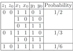
Suppose there were no carry into the addition window. Ten of the sixteen possible input combinations produce this result. The possible values for (z0, z1) are found in table 1, along with the probability of occurrence and the operands that produce each of the values. The distribution is clearly no longer uniform, and is biased towards larger values.
z1z0x1x0y1 y0Probability
0 0 0 0 0 0 1/10 0 1 0 0 0 1 2/10
0 1 0 0
1 0 0 0 1 0 3/10 0 1 0 1
1 0 0 0
1 1 0 0 1 1 4/10 0 1 1 0
1 0 0 1 1 1 0 0
Table 1. Possible values for bits ofx, y,and z preceding the target windowz(2) - no carry into addition window
z1z0x1x0 y1 y0Probability
0 0 1 1 0 1 1/2 1 0 1 0
0 1 1 1
0 1 1 1 1 0 1/3 1 0 1 1
1 0 1 1 1 1 1/6
Table 2. Possible values for bits ofx, y, andz preceding target windowz(2) - carry into addition window
Now suppose that there was a carry into the addition window. Six operand combinations produce this result. The possible values for (z0, z1) are found in table 2, along with the probability of occurrence and operands that produce those values. Again,z0 andz1do not belong to the uniform distribution. Unlike the previous case, the values are now biased towards smaller values.
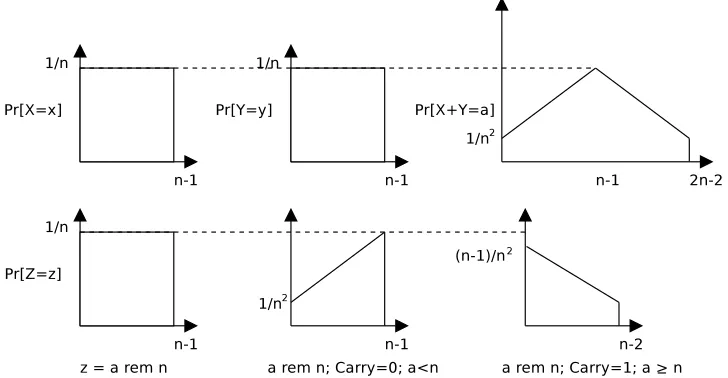
This can be understood more generally as follows. If integer addends X and Y, both in [0, n−1], are added, the distribution of the result is the discrete convolution of the distributions ofX andY, and it takes on values in [0,2n−2]. Further, if the distributions on X andY are both uniform, then the probability of the sum increases linearly from its smallest value of n12 at the value 0 to a maximum atn−1 and then decreases linearly to n12 at the maximum value of the sum, 2n−1. This may be understood by noting that many combinations of valuesxandyof the addendsX andY will give a sum ofn−1, while only one pair of
Fig. 2.Carries and addend distribution
3.2 Creating Approximations
Three aspects of the pseudo-linear approach are important.
Base Approximation The simplest approximation is formed by deriving the target window in terms of all
the windows it depends on. All exclusive-or operations are preserved. Addition modulo 2n operations are preserved as well, but the addends are incomplete. After each addition, bits outside the active windows are cleared (set to zero). For each unknown carry into a window, no carry is assumed.
Carry Patterns A carry pattern is a series of carry values,ci∈ {0,1}, where eachidenotes an approximated
addition window that may have a carry into it. Stated differently, there is a ci for every approximated addition window that does not start with the least significant bit of the word. One can construct multiple carry patterns that overlay the base approximation such that 1 is added to approximated addition window
iifci= 1. LetCj= (c
0. . . cm−1) represent the carry pattern formapproximated addition windows. Then each base approximation overlaid with a distinct carry pattern, base+Cj, represents a distinct approximation. By applying several carry patterns to the same input/output pairs and obtaining several likely approximations, one can increase the probability of hitting upon the correct one, which in turn increases the bias.
The best carry pattern for a particular set of plaintexts depends on the input distribution. For example, the carry pattern for low Hamming-weight inputs will have fewer carries than for high Hamming-weight inputs. Note that this knowledge could potentially be used to find the Hamming weight of keys.
Offsets Another method of compensating for mispredicted carries is through the use ofoffsets. Recall that
−20 −10 0 10 20
0.00
0.01
0.02
0.03
0.04
offset
Pr[appro
x+offset = actual]
w=8
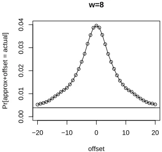
Fig. 3.An example: observed probability of correctly guessing window of ARX target over several offsets. Plot created with window isolation (section 3.4), the base approximation presented in section 6.1, andw= 8. Further details in section 6.
Computing Bias The improvements outlined above increase the probability of the approximation being correct, but also increase the probability of guessing correctly at random. That is, a random guess with
cpdifferent carry patterns will be correct with probability 2cpw instead of
1
2w since each pattern represents a
different approximation. Therefore, we need to adjust the bias calculation when using multiple carry patterns and/or offsets. LetT be the number of times the guess is correct, andPbe the number of plaintext-ciphertext pairs. Letcpbe the number of patterns used, and letf be the offset. Then the bias is calculated according to equation 1.
bias=T−cp(2f + 1)
2w P (1)
3.3 Comparison to Linear Cryptanalysis
The main advantage of pseudo-linear cryptanalysis when compared with linear cryptanalysis is that it allows the adversary to create approximations that have higher bias than those that could be achieved by only considering approximations in the boolean vector space.
Another significant advantage is that pseudo-linear analysis leads to flexible approximations. Once a base approximation has been established, it can easily be modified through the use of offsets and carry patterns to accommodate different scenarios. For example, a change in the input distribution does not require a change to the base approximation, only a change to the carry pattern and/or offsets. It is also trivial to change the window size, since only the position of the least significant bit of the window is important. The most significant bit can be computed dynamically based on the desiredw.
provide the weakest assistance. The larger wis, the less accurate approximating addition modulo 2w with exclusive-or (or visa versa) becomes.
3.4 Implementation Methods
There are two implementations of pseudo-linear approximations over ARX functions that are demonstrated here.
1. Each window stored in its own word (window isolation)
2. All windows for a word stored in the same word (word isolation)
The first is useful for developing approximations, but the latter is much better in practice. This is because the first case provides a way to isolate windows that simplifies the debugging process. However, when windows are adjacent or overlap, there is carry information that is not used due to the high level of isolation. It also becomes possible for a single bit to take on multiple values in multiple windows, which is clearly not correct and will reduce the bias. In the second method, bits may no longer take on multiple values, and the attacker can take advantage of the extra carry information to obtain stronger biases.
The first approach also has another drawback. Because there is an addition performed for each addition window, the number of additions increases rapidly with each round. The second method uses at most twice the number of additions (1 for word addition, 1 for carry addition).
It is also essential that window position is preserved. When an addition is performed on windows that wrap around a word, it is important that the carry out of positionn−1 isnot propagated. Both implementation methods respect this. We stored windows in 64-bit words (regardless of isolation) in the following manner. The bits in a window were set to their correct value in the corresponding position, and all other bits set to 0. Let x(i) indicate the window beginning at position i in word x, and consider 64-bit words. With window isolation,x(8) =0x2E would be represented as 00000000 00002E00, and all other windows would have their own distinct 64-bit word. With word isolation and two 16-bit windows,x(8) = 0x5678 andx(40) = 0x1234, the word would be represented as 00123400 00567800.
When using word isolation, the inactive bits may all be set to zero after each addition. Alternatively, they may remain after all operations, and be used throughout the cipher. The latter may be difficult to implement correctly depending on the method of deciding whether or not to add 1 when a carry is guessed. The first approach has been found to be more beneficial overall, although there were drops in bias at certain
wvalues.
4
Truncated Differentials
Pseudo-linear methods are directly applicable to truncated differential attacks. A typical differential attack relies on differential characteristics, which are sequences of input and output differences over one or multiple rounds. A differential trail can be created by chaining characteristics to cover more rounds.
Pseudo-linear approximations can be used to discover differential trails – particularly truncated differen-tial trails. Unlike a traditional differendifferen-tial which uses the entire state, a truncated differendifferen-tial works with a portion of the state. A common practice in differential calculation is to linearize the function (replace addi-tion/subtraction modulo 2n with exclusive-or). We propose to eliminate the linearization step and instead follow the differentials in windows.
Lemma 4. Letx and x′ be two n-bit words, x′⊕x=δ, x > x′.Letw be the window size in bits. Then Pr[part(x−x′, s,(s+w) modn) =part(x, s,(s+w) modn)⊟
wpart(x′, s,(s+w) modn)]> 12
Proof. This follows directly from Corollary 2.
1 0
1
<<< 0
1
1
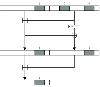
Fig. 4.Simple view of tracing differences
of addition, rotation, and exclusive-or, there is a 1-bit difference in the left window and in the right window, with some probability. After another addition, there is still a 1-bit difference, with some probability.
The differences can be traced from word to word throughout the function. How a difference in the input affects each window in the trace depends on the location of the differences relative to the windows. In particular, a difference occurring in less significant bits than a window has less impact as the distance between the start of the window and the difference increases. This is because the probability of the difference introduced by the carry function propagating to the window decreases as the distance between the difference and the window increases.
Consider the example in figure 4, but allow the possibility that there are differences outside the window which are possibly unknown. If the input difference of the left word is 11112, the difference of the addition will propagate differently than than if the input difference is 10002. If the window begins at the fourth least significant bit, then both result in a differenceinside the window of 1, but the differencesbefore the window produce different carry distributions, thereby affecting the difference propagation inside the window. If the window begins much farther away from other differences, then the impact will be smaller. For example, if the window began in position 32, and the difference outside the window only occurred in the least significant bit, then the probability of that difference affecting the window after one addition is much smaller because the probability of the carry function reaching that far is much smaller.
4.1 Difference in Addition
We now investigate how different operators affect the trail. First, consider how differences affect the approx-imation addition modulo 2w.
Difference in one addend Let us start by considering twon-bit words,xandx′,x′=x⊕1, and a third wordy. Whenz=x⊞y and z′ =x′⊞y, there is a difference in the first addend, but there is no difference in the second addend. We can say something about the resulting differencez⊕z′.
The simplest claim we can make is that the last bit ofz⊕z′ is the same as the last bit ofx⊕x′. When
x⊕x′ is even, this claim is straightforward. Whenx⊕x′ is odd, this may be deduced as follows. Without loss of generality, letxbe even andx′ be odd, such thatx⊕x′ is odd. Ify0 (the least significant bit ofy) is 0, thenz0= 0 and z0′ = 1. If y0= 1, thenz0= 1 and z′0= 0. In both cases,z⊕z′= 1.
More interesting to consider is how carries propagate. In particular, there are cases where strings of ones can be created or broken due carries. To see this, let us examinez′. Supposex⊕x′ = 1 and thatyis selected from the uniform distribution at random. Then pr[z′0 = 0] = 21. If y0 = 1, then carry0 = 1 and z
If the input difference has a run of multiple ones (e.g. 3, 7, F, but not 1), some of the ones may turn to zeros in the output difference. For example, letx= 11112andx′= 11002, givingx⊕x′= 112. Lety= 11012.
1 1 1 1 1 1 0 0
⊞1 1 0 1 ⊞1 1 0 1
1 1 0 0 1 0 0 1
Forx⊞y, carries result from positions 0, 1, and 2. Forx′⊞y, carries result from position 2 only. The resulting difference characteristic here is∆= 00112→δ= 01012, and the string of ones is broken.
In both addends It may be the case that both addends have difference patterns. For example, letx′=x⊕∆, andy′=y⊕Γ. Addition is performed asz=x⊞y, andz′=x′⊞y′, and z⊕z′=δfor some valueδ.
While the structure of the output difference is going to vary greatly by input differences, one can easily say something about the least significant bit of the difference pattern.
Consider some difference pattern 000XXX000 in ∆ and Γ where X marks a possibly nonzero difference.
Since there is no difference coming into the bits marked byX, the carry function into that region behaves the
same way in both additions. Therefore we eliminate the zero regions from consideration and only consider
XXX. One can say something about the least significant bit of XXXbased on the least significant bit of the
input difference patterns.
Lemma 5. If both inputs have an even (odd) difference pattern, then the sum will have an even difference pattern. If one input has an odd difference pattern and the other an even difference pattern, then the sum will have an odd difference pattern.
Proof. Let the functionlsb(d) return the least significant bit of the difference window. If the difference in
both input windows is even,lsb(x) =lsb(x′) andlsb(y) =lsb(y′). Hence,
lsb(z)⊕lsb(z′) = (lsb(x)⊕lsb(y))⊕(lsb(x′)⊕lsb(y′)) = (lsb(x)⊕lsb(x′))⊕(lsb(y)⊕lsb(y′)) = 0 Now suppose the difference in both input windows is odd, solsb(x) =lsb(x′) andlsb(y) =lsb(y′). Hence,
lsb(z)⊕lsb(z′) = (lsb(x)⊕lsb(y))⊕(lsb(x′)⊕lsb(y′)) = (lsb(x)⊕lsb(x′))⊕(lsb(y)⊕lsb(y′)) = 1⊕1 = 0 Finally, suppose one addend has an odd difference pattern and the other an even difference pattern. Without loss of generality supposelsb(x) =lsb(x′) andlsb(y) =lsb(y′). Hence:
lsb(z)⊕lsb(z′) = (lsb(x)⊕lsb(y))⊕(lsb(x′)⊕lsb(y′)) = (lsb(x)⊕lsb(x′))⊕(lsb(y)⊕lsb(y′)) = 0⊕1 = 1
4.2 Difference in Exclusive-Or
When a difference occurs in only one of the operands, that difference is preserved by exclusive-or. Consider
n-bit wordsa,a′=a⊕∆, andb, and letc=a⊕bandc′=a′⊕b. Thena′⊕b=a⊕∆⊕b→c′⊕c=∆.
4.3 Differences Over Round Functions
The simplest cases to analyze are those with low Hamming weight differences. Consider x′ = x⊕2i, i ∈
{0, . . . , n−1}.
4.4 Windows and Truncated Differentials
A differential trail, truncated or otherwise, typically coversr−1 ofrrounds. The adversary chooses inputs
P andP⊕∆, and receives their encryptionsC andC′. Next, the adversary guesses portions of the key that are needed to compute the target window (where the target difference occurs), and backs up one round to obtainT andT′. IfT⊕T′ =δ, whereδis the target difference, then increment a counter for those key bit values. At the end, the guessed key bits that producedT ⊕T′ =δ at the expected rate are the most likely candidates.
Windowing is used differently for differentials than for pseudo-linear approximations. This is because higher accuracy is required when working with differentials. Specifically, target windows should be formed such that no subtraction is left to chance. The word should be covered from the least significant bit to the highest position across all relevant windows so that all borrows are known.
One strategy is to start with small windows, sayw= 4. Once all the bits involved with that window size have been found, increasew. The window position does not change, but more of the unknowns are slowly added to the windows. This proceeds until allnbits of a key word are active and the entire word has been guessed,or the correct key is no longer distinguishable from incorrect keys. This can happen if all the new key bits guessed do not change the probability of resulting in the target difference. Note that the difference in a word is the difference over the entirenbit word, where inactive bits are zero.
5
Evaluating ARX Functions
Diffusion in ARX is achieved primarily through rotation, and secondarily by the carry function of the addition. There is little work which describes how to construct a good round function, and how to determine how good an existing round function is.Branch number is a metric currently in use, and was used in the design strategy for the Advanced Encryption Standard (AES) [7].
5.1 Branch Numbers
The differential branch number and linear branch number metrics are measures of diffusion that apply to any mapping. Here, their use is restricted to the context of key-alternating round functions. Branch numbers provide lower bounds for the amount of diffusion in a round function, allowing simpler analysis of the weight (or probability) of a trail over several rounds. The metrics have been defined for any partition [6], as well as a specific type of partition [7]. In [7], branch numbers are defined as part of anm-bit partition of the state, consisting ofbundles. Bundles are adjacent and do not overlap, such that the state is divided intonbbundles andnbmis the size of the state in bits.
A bundle is called active when it is part of a differential or linear trail. That is, when a difference or selection pattern is non-zero for that bundle in a differential or linear trail, respectively. Thebundle weight
of a state is defined as the number of active bundles in that state. The bundle weight of state ais written
wb(a).
Branch number metrics are defined differently for differential and linear trails [7]. As the number of rounds increases, the branch number becomes more complex and difficult to reason about. However, it has been shown that properties of round functions can be derived by looking at two-round trails, and viewing 2rrounds as a sequence ofrtwo-round trails[7]. Therefore, only two-round trails will be discussed here.
For input vectorsaandb, the differential branch number for round transformationφis defined as [7]:
Bd(φ) = min
Linear branch number is similar. For an input selection patternα, output selection patternβ, correlation functionC(.), and inputx, the linear branch number of a round transformationφis defined as [7]:
Bl(φ) = min
α,β,C(αTx,βTφ(x))6=0{wb(α) +wb(β)} (3)
Generally speaking, this is the minimum of the sum of bundle weights for the inputs and outputs ofφover all selection masks, where the active input and output to theφfunction are correlated.
Branch Numbers in ARX This metric works well for states that are comprised of a sufficient number of bundles. However, diffusion in ARX round functions comprised of few large bundles (e.g., four 32-bit or 64-bit words) may be difficult to accurately capture with this metric.
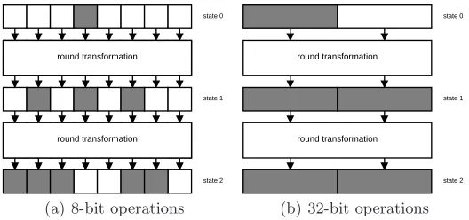
To see why, consider the scenario in figure 5, where two round transformations have approximately the same amount of diffusion, but one round function is an SPN that operates on bytes (figure 5(a)) and the other is an ARX function using 32-bit words (figure 5(b)). In both round functions, the same bits are part of a linear or differential trail. Portions of the state (byte or word) that contain at least one bit of the trail are called active, and are colored grey in figure 5. When operations are performed in 32-bit words, each word covers four bytes. As a result, all of state 1appears active in 5(b), whereas only 3
8 of state 1is active in 5(a). Similarly, 58 of state 2is active in figure 5(a), while again being completely active in figure 5(b). In
this example, it appears that the diffusion is far better in 5(b), when it really is not. A state composed of few large words can produce branch numbers that are misleading.
round transformation
round transformation
state 0
state 1
state 2
(a) 8-bit operations
round transformation
round transformation
state 0
state 1
state 2
(b) 32-bit operations
Fig. 5.Trail in two transformations with approximately the same amount of diffusion
We propose two approaches to more accurately measure diffusion in this type of round function. The first proposal is based on the idea of breaking large words into smaller ones, and modeling addition as data dependent substitution boxes. The second approach leverages concepts of pseudo-linear analysis.
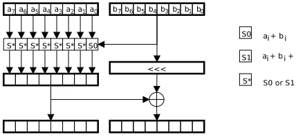
S-Box Representation Addition modulo 2n can be represented as a series of smaller data-dependent substitution boxes, as shown in figure 6. There are two kinds of S-boxes:
S0: ai=ai+bi
S1: ai=ai+bi+ 1
Fig. 6.S-box representation of an ARX function Fig. 7.Threefish mix function; rotation varies by state and position
A bundle is not considered active in a differential trail unless there is a non-zero difference in the input to the corresponding S-box. That is, if there is a non-zero difference in the input of an S-box step, but one input is toS0and the other is toS1, the bundle willnot be considered active. The rationale for this is that branch number provides a lower bound, so only the minimum number of S-boxes affected is considered here.
Alternate Metric Pseudo-linear analysis lends itself to another possibility for application of the branch number metrics. If the restriction that bundles be non-overlapping adjacent portions of the state were re-moved, then bundles would strongly resemble windows in a pseudo-linear system. In fact, when this restriction is removed, pseudo-linear approximations are directly applicable to the bundles to trace dependencies and influence. It is this idea that motivates an alternate metric for diffusion in ARX rounds, called effective
branch number.
The very first step is to determine the proper window (bundle) size. In pseudo-linear cryptanalysis, the bounds on window sizew are defined as 1≤w < n.
Just as the original branch number metrics used bundle weight, these variants useeffective bundle weight, denotedewb. Effective bundle weight is calculated as the ceiling of the total number of active bits divided by the bundle size.
Example 1. Consider a round function and approximation with five active input windows, but all five
win-dows start one bit off from another. That is, we have winwin-dows starting in positionsi, i+ 1, i+ 2, i+ 3, and
i+ 4. The only bits that are not contained in multiple windows are the first bit of windowx(i) and the last bit of windowx(i+ 4). The bit range covered by these windows is [i . . . i+ 4 +w). The number of state bits in this range is 4 +w.
Ifw= 2, then the effective bundle weight is⌈62⌉= 3. Ifw= 4, then the effective bundle weight is⌈84⌉= 2. Ifw= 8, then the effective bundle weight is⌈128⌉= 2.
The definitions for linear and differential effective branch number are simple extensions of the branch number metrics from [7]. They only differ in that effective bundle weight is used in place of bundle weight. We denote the differential effective branch number as EBd and pseudo-linear effective branch number as
EBpl.
Over two-round trails, the differential effective branch number of a transformationφis derived by equation 4. Recall from equation 2 thataandbare input vectors to the first round, andφ(a)⊕φ(b) is the difference at the input to the second round.
EBd(φ) = min
a,b6=a,w{ewb(a⊕b) +ewb(φ(a)⊕φ(b))} (4) Similarly, the pseudo-linear effective branch number of a transformationφis derived by equation 5. The selection mask of the input to the first round is α, the selection mask at the input to the second round is
EBpl(φ) = min α,β,C(αTx,βT
φ(x))6=0,w{ewb(α) +ewb(β)} (5) The matter of selecting an appropriatew has yet to be addressed. The minimum useful window size is that which allows a round function to be distinguished from a random permutation. This in turn depends on the number of additions required to compute a target window, denoted by n⊞. If windows do not overlap, then the effective branch number should be equivalent to the branch number calculations of [7]. To satisfy this requirement,wshould divide the number of bits in the state. Thus, for state width that is a power of 2, letw= 2⌊lg(n⊞)⌋. Note that only the additions occurring in the key-independent portion of a round function should be used to derive the appropriatew.
6
Application: Threefish
Threefish[8] is the tweakable[17] block cipher inside the compression function of SHA-3 finalist Skein[10]. Two variants are discussed here: Threefish-256 and Threefish-512. The state and key are comprised of 64-bit words, where there are B bits in the state and the key of Threefish-B. The cipher consists of 72 rounds, where each round contains two main steps: mix and permute.
The mix function, shown in figure 7, is an ARX function where addition is performed modulo 264 and the rotation depends on the mix inputs and round. Each mix is numbered by 0, 1, 2, or 3, where each is computed asmix0(x0, x1), mix1(x2, x3),mix2(x4, x5), andmix3(x6, x7), in Threefish-512. Threefish-256 requires onlymix0(x0, x1) andmix1(x2, x3).
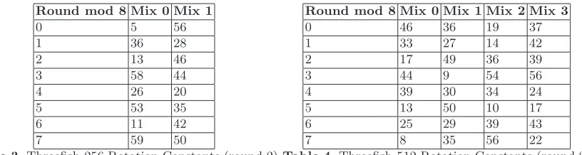
The rotational values for each mix in each round can be found in tables 3 and 4.
Round mod 8 Mix 0 Mix 1
0 5 56
1 36 28
2 13 46
3 58 44
4 26 20
5 53 35
6 11 42
7 59 50
Table 3.Threefish-256 Rotation Constants (round 2)
Round mod 8 Mix 0 Mix 1 Mix 2 Mix 3
0 46 36 19 37
1 33 27 14 42
2 17 49 36 39
3 44 9 54 56
4 39 30 34 24
5 13 50 10 17
6 25 29 39 43
7 8 35 56 22
Table 4.Threefish-512 Rotation Constants (round 2)
The permutation step of the round function is straightforward. Each 64-bit word is mapped to another position according to the mapping,π, given in table 6. That is,xi ←xπ(i).
i 0 1 2 3 π(i) 0 3 2 1
Table 5.Threefish-256 Permutation,π
i 0 1 2 3 4 5 6 7 π(i) 2 1 4 7 6 5 0 3
Table 6.Threefish-512 Permutation, π
words store information about what has been done so far (bits processed, level in the hash tree, etc.). No structure of the tweak words is assumed when the cipher is considered on its own.
The Threefish key schedule is given by equations 6-9, where constant is a constant that was changed between the first [8] and final [10] submissions to NIST. For the purpose of this work, the value of the constant is not relevant1. Therefore, it is left as a variable to include all submitted versions of the algorithm.
RKiis round keyi∈ {0, . . . ,18}, whereRK0is the whitening key. Each round key is derived from theN+ 1 key words (denotedkj,j ∈ {0, . . . ,8}) and three tweak words (t0, t1, t2).
kN =constant⊕ N−1
M
i=0
ki (6)
t2=t0⊕t1 (7)
Round keyifor Threefish-256 is derived by
RKi=kimod 5||k(i+1) mod 5+timod 3||k(i+2) mod 5+t(i+1) mod 3||k(i+3) mod 5+i (8) Similarly, the key schedule for Threefish-512 is expressed by
RKi=kimod 9||k(i+1) mod 9||k(i+2) mod 9||k(i+3) mod 9||k(i+4) mod 9 (9)
||k(i+5) mod 9+timod 3||k(i+6) mod 9+t(i+1) mod 3||k(i+7) mod 9+i
6.1 Pseudo-Linear Attacks on Threefish-256
Approximation Over Modified 8 Rounds The application of pseudo-linear attacks to a modified version of Threefish-256 is presented in this section. The modified version has a fixed tweak schedule of zero, is reduced to 8 rounds, and does not include the injection of a whitening key. This approximation covers the modified cipher from the key injection of round 4 to the key injection at round 8, inclusive.
Let xi denote the ith word of the plaintext and x j i the i
th word after round j. Let xj
i(m) denote the window of wordxji with its least significant bit in positionm. That is,x
j
i(m) =part(x j
i, m,(m+w) mod 64). When a single word contains multiple active windows, a0. . . am, let x
j
i(a0, . . . , am) be the same as
xji(a0), . . . , xji(am).Ki(m) denotes the window starting at positionmof theithword of the key schedule. The approximation forx8
0(0) is presented in figure 8. The active addition windows are listed to the upper left of each⊞symbol. rotl(r) represents a left rotation byrbits of a 64-bit string.
Computations before the fourth round key addition can be performed by following the cipher operations, and are not included here. The number of key bits needed in this approximation depends on the window size. For example,w= 3 requires 58 key bits,w= 4 requires 75 key bits, andw= 5 requires 92 key bits.
Empirical results for bias were obtained with varying window sizes, using 20,000,000 pseudorandomly generated (data, key) pairs and tweak schedule fixed to 0. This methodology is based on the one used in the original Skein submission to the SHA-3 competition [8], where differential biases were computed using 20,000,000 pseudorandom (data, key, tweak) tuples.
As mentioned in section 3.4, there were two methods of implementation used – the less efficient and less accurate but easier to debug window isolation, and the more accurate and more efficient but more difficult to debug word isolation.
For simplicity, a carry patternCi is represented as an arrayCi
jk, wherej is the round number andk is the word number. In these experiments, if a wordkof roundj contained multiple windows, the same carry guessCi
jk was applied to all of those windows.
1
Fig. 8.Approximation forx8
0(0), without whitening
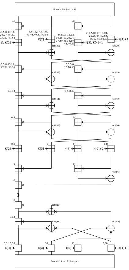
Fig. 9. Approximation for 12 rounds, meeting at x10
0 5 10 15 20 25 30 35 0 0.1 0.2 0.3 0.4 0.5 0.6 w Observed bias offset=0 offset=1 offset=2 offset=3
offset=0 (WRONG KEY) offset=1 (WRONG KEY) offset=2 (WRONG KEY) offset=3 (WRONG KEY)
Fig. 10. Base approximation with window isolation, x8
0(0)
0 5 10 15 20 25
0 0.1 0.2 0.3 0.4 0.5 0.6 0.7 0.8 0.9 1 w Observed bias cp0 (base) cp1 Both cp
Both cp (WRONG KEY)
Fig. 11.x8
0(0) approximation with word isolation and
different carry patterns (cp)
Figure 10 demonstrates the effect of offsets on an approximation, with both the correct and incorrect key values, where observed bias is computed according to equation 1. Offsets increase the probability of correctness for wrong values considerably because they also result in larger solution sets. On the other hand, correct values continue to have a higher bias on average. The same is true when multiple carry patterns are used, and the resulting solution set consists of all the solutions resulting from the carry patterns used. Figure 10 also shows that there is a maximum bias that can be achieved with window isolation, where the maximum probability of correctness is strictly smaller than 1.
Figure 11 presents some results obtained using word isolation and offset=0. It demonstrates that word isolation provides better results, as expected, and that the correctness probability grows to 1 aswincreases. This causes the bias to approach 1, since the probability of correctness for a random guess drops closer to zero as w increases. Finally, it shows how different carry patterns can affect the approximation. The two carry patterns used here were:
Cj0k= 0, Cj1k=
0 ifj is even 1 ifj is odd
When a large enough number of key bits is to be guessed, the bias values for different carry patterns converge (here, this happens atw= 12). If multiple carry patterns are used together, as they were here, the resulting bias may be smaller than the bias obtained by using a single, stronger carry pattern.
Approximation Over Modified 12 Rounds The application of pseudo-linear attacks to a modified version of Threefish-256 is presented in this section. The modified version has a fixed tweak schedule of zero, is reduced to 12 rounds, and does not include the injection of a whitening key. This approximation covers the modified cipher from the key injection of round 4 to the key injection at round 12, inclusive.
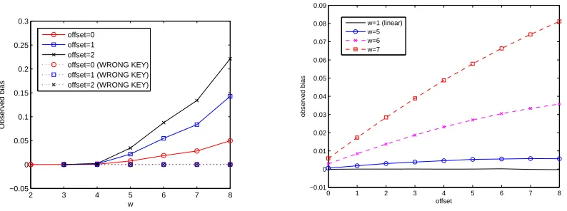
Figure 12 contains results from the 12 round approximation with carry patternC1 and different offsets using word isolation. It shows that the correct key bits are indistinguishable forw <5. Withw= 5, 232 of 256 bits of key are involved in the approximation.
To demonstrate key recovery using pseudo-linear approximations, a smaller attack was performed with the 8 round approximation forx8
2 3 4 5 6 7 8 −0.05
0 0.05 0.1 0.15 0.2 0.25 0.3
w
Observed bias
offset=0 offset=1 offset=2
offset=0 (WRONG KEY) offset=1 (WRONG KEY) offset=2 (WRONG KEY)
Fig. 12.Bias Threefish-256 12 round approximation
0 1 2 3 4 5 6 7 8
−0.01 0 0.01 0.02 0.03 0.04 0.05 0.06 0.07 0.08 0.09
observed bias
offset w=1 (linear)
w=5 w=6 w=7
Fig. 13.Observed bias for Threefish-512 8 round dis-tinguisher
Ifw= 3, then the attack on 11 rounds requires 58 bits of key (as compared to 256 bits for a brute force attack) to be guessed. Without expending too much energy on computation, in order to observe the kinds of errors that might result, we attempted to determine 18 key bits assuming that the other 40 were known. Because the carry function is difficult to determine with incomplete knowledge of the operands, the correct value of the key is not always among the top few candidates. In these experiments, the goal was to eliminate 90% of the possible key values, with the correct value in the remaining 10%. We ran 500 independent key recovery attacks, each with a pseudorandomly generated key and 10,000 pseudorandomly generated plaintexts. The results are summarized in table 7, where we note when the correct key value has the maximum bias, as well as when the correct value is in the top 10% of key estimates ranked by bias.
offset=0 offset=1 offset=2 offset=3 correct 11% 12.2% 14.4% 7.2% in top 10% 92.6% 97.4% 96.8% 92.2%
Table 7.500 attacks, 10,000 pairs
Key Recovery These approximations can be used for key recovery with known plaintext and ciphertext. Because there is no key injection in rounds 15 through 13, the output of round 15 can be decrypted to derive the output of round 12 correctly. The input up to the fourth round key injection can also be computed precisely because the modified cipher does not include the whitening key injection. In this scenario, the 12 round approximation could be used to determine some of the key bits from 15 rounds.
0 1 2 3 4 5 6 7 −1.5
−1 −0.5 0 0.5 1 1.5 2 2.5
3x 10
−4
offset
observed bias
w=4 w=5 w=4 (wrong key) w=5 (wrong key)
Fig. 14.Observed bias for 12 round Threefish-512 dis-tinguisher, random messages
0 1 2 3 4 5 6 7
−0.005 0 0.005 0.01 0.015 0.02 0.025 0.03 0.035
offset
observed bias
w=3 w=4 w=5 w=4 (wrong key) w=5 (wrong key)
Fig. 15.Observed bias for 12 round Threefish-512 dis-tinguisher, low Hamming weight messages
6.2 Pseudo-Linear Attacks on Threefish-512
In the previous two attacks, a modified Threefish-256 was used where the whitening step was eliminated. In the following approximations, the only modification made is the number of rounds. That is, the first key injection considered is the key whitening.
Approximation Over Modified 8 Rounds An 8-round approximation was constructed with a meet-in-the-middle approach. It meets at word 1 at the end of the fourth round. The addition (subtraction) windows for this distinguisher are presented in Appendix A, table 13. There are no subtraction windows in the fifth round because no subtractions are needed to obtainx41(0).
Empirical results for this distinguisher are presented in figure 13. These results were obtained using 20,000,000 randomly chosen (plaintext, key) pairs with the carry pattern where carries are assumed every other round. It is clear from the plot that eight rounds of Threefish-512 are distinguishable forw≥5.
The number of key bits required by this distinguisher for window sizes w= 5,w= 6, andw= 7 are 310, 355, and 391, respectively. Recall that for a distinguisher from Threefish-256, eight rounds withw= 5 (seen in the modified 12 round distinguisher, section 6.1) required 232 of the 256 bits, or about 90%. In this eight round distinguisher for Threefish-512, a window size of 5 requires only about 60% of the 512 key bits to be guessed. The principal reason for this is that with the increased state size, diffusion between words is slower. Specifically, it takes more applications of the permute function, and therefore more rounds, to mix all eight state words.
12 Round Approximation A 12-round approximation can be obtained in a similar fashion to the 8 round one. In particular, one was constructed that meets in the middle at word 1 of the seventh round. The addition (subtraction) windows for this distinguisher are presented in Appendix A, table 14.
The key bits that need to be guessed forw= 4 and w= 5 are 509 and 511, respectively. Beyond that, all 512 bits need to be guessed for this distinguisher.
Empirical results are presented in figure 14 and 15 for two different plaintext selection criteria. In figure 14, 20,000,000 (plaintext, key) pairs are chosen at random. The alternating carry pattern was used. In figure 15,keyis still chosen at random, but the plaintexts are chosen such that they have a hamming weight of 1. For each randomly selectedkey, 512 plaintexts are used. Carries are assumed in rounds 6 and 8.
Figure 14 shows that one cannot effectively distinguish the correct key from incorrect keys whenw≤5 and plaintexts are selected at random. Whenw >5, all 512 bits need to be guessed.
be distinguished from a random permutation withw= 4 and offset≤6. However, it cannot be distinguished from a random permutation forw≤3, so 509 bits is the minimum that must be guessed for this distinguisher.
6.3 Truncated Differentials for Threefish-512
In this section, we construct a truncated differential attack on four rounds of Threefish-512. This is a single-key chosen-plaintext attack with a pre-determined difference between pairs of plaintexts. The focus is on differences in window bits. Differences in bits outside the window are ignored.
Let the input bex′
0=x0⊕1,x′i=xi fori∈ {1. . .7}, and the target window bex33(55). The size of the window will begin small, such asw= 4, and then increase as the adversary gains more information.
The target window location is not arbitrary. Recall from section 4.4 that we need to remove uncertainty introduced by the carry by working with the least significant window for all subtractions. Since there is a right rotation by 9 after the key subtraction, we have (0−9) mod 64 = 55, so the target window for x33 starts at position 55.
To see how the target window is affected by the input difference, it is helpful to observe how the difference propagates through the trail forx33. The first three rounds of Threefish-512 are shown in figure 16. The trail is marked with thick arrows.
Fig. 16.Three rounds of Threefish-512
First Round The first round begins with the key whitening. The same key will be added to both plaintexts,
xandx′, which are equal except in the least significant bit of word 0. Words 1 through 7 have no difference before and after the key injection.
In word 0, after key injection, the difference will consist of a string of n−t zeros followed by t ones, 1≤t≤n. The reason for this is as follows (recall section 4.1). Without loss of generality, letx0be even and
x′
0 be odd. Thenx0⊞k0=x∗0 will not cause a carry out of position 0 regardless of the value ofk. If the least significant bit ofk0 (denote this as k0[0]) is 0, then x0′∗[0] = 1. Ifk0[0] = 1, thenx′∗0[0] = 0. Assuming that
kis selected from the uniform distribution at random, then pr[x∗
0[0] = 0] = 12. Ifk0[0] = 1, thencarry0 = 1 andx′∗
0[1] =x∗0[1]. This continues untilcarryt−1= 0. Bits in positiont, . . . , n−1, are identical inx0andx′0 and thus the run of ones ends at aftert bits.
Word Input difference (∆x0) Output difference (δ)P r[δ|∆x0] (approx)
x∗ 0
1 2−1
3 2−2
1 7 2−3
F 2−4
1F 2−5
Table 8.Key whitening difference probabilities
The first key injection is followed by the mix and permute steps. Recall that Threefish-512 computes four mix functions in parallel, where each mix function consists of an addition, word rotation, and exclusive-or. After mix function i ∈ {0,1,2,3} has been applied to words 2i and 2i+ 1, the words of the state are permuted to facilitate diffusion. There is no difference between words 1 in the two texts before the addition of the mix, but the words 0 differ by a string of ones. The rotation is performed on words 1, but there is no difference between them and thus there is still a zero difference after rotation. The final step of the mix is the exclusive-or of the rotated words 1 and result of the addition modulo 2n. As a result, the words 0 still differ by a string of ones after the mix, and this string of ones is also the difference between the words 1 after the mix because these words differ from the corresponding words 0 only in that they are xored with the same string.
Permutation does not change the value of a difference within a word, only the word that it appears in. In particular, the string of ones forming the difference in word 0 after the mix step moves to word 6 after permutation, and the zero difference in word 2 moves to word 0 (see table 6). Word 1 maps to itself during this step, so at the end of round 1, the only non-zero difference bits are in words 1 and 6.
Some of the higher probability characteristics are summed up in table 9. These probabilities are dependent on the input difference to the first round mix function. That is, they are conditional probabilities where the result depends on the difference after the whitening step.
Second Round The incoming differences are inx1
6 andx11.x16 will affect output windowsx24 because word 6 will be permuted to word 4 after the addition, andx2
3 because word 7 will be swapped with word 3.x11will affectx2
6as in the first round, because the zeroth word is permuted to the sixth position, and the first word is not affected by the permutation, andx21. However,x21,x23, and x24 are not in the dependency path forx33, as can be seen by following the wordsx33is derived from, and can be ignored for this differential. This leaves onlyx26.
x26 (derived fromx10 andx11) is interesting because the format of the words is different from those we’ve seen before. In previous rounds, the differences in the left words have been strings of ones, but neither of the texts, at this part of the cipher, themselves contained the difference runs in the corresponding words. For example, a difference of 3 would be achieved by having the least significant bits 012in one word and 102 in the other. In the input word x11, one of the words contains the difference. That is, one word contains∆x1 1 in the least significant bits, while the other contains zeros. For a difference of 3, this would be 112 in one word and 002 in the other. Section 4.1 showed how the run of ones in the difference pattern can break in this scenario. Because of this, differences that are not runs of ones are possible, such as0x05and0x0B.
Third Round Only one word in the trail has a difference into round 3:x26. x26 affectsx33.
Again, a difference in the right input creates more interesting transitions. The output difference proba-bilities forx33 do not all contain perfect powers of 2 in the denominator. A subset of the possible transitions is shown in table 10.
We have showed the effect of the input difference throughout three rounds of a trail. This information can be used to construct a truncated differential attack on four rounds.
Word Input differ-ence (∆x∗
0)
Output differ-ence (δ)
P r[δ|∆] (approx)
x1
6 andx
1 1
1 2−1
3 2−2
1 7 2−3
F 2−4
1F 2−5
1 2−1
3 2−2
3 7 2−3
F 2−4
1F 2−5
1 2−1
3 2−2
7 7 2−3
F 2−4
1F 2−5
1 2−1
3 2−2
F 7 2−3
F 2−4
1F 2−5
Table 9.Round 1 difference probabilities
Word Input differ-ence (∆x26)
Output differ-ence (δ)
P r[δ|∆] (approx)
x3 3
1 2−1
3 2−2
1 7 2−3
F 2−4
1F 2−5
1 2−1.32
3 2−2
5 2−4.32
3 7 2−3
D 2−5.32
F 2−4
1D 2−6.32
1F 2−5
3 2−2.32
5 2−2
7 2−3
5 D 2−3
F 2−4
1B 2−6.32
1D 2−4
1F 2−5
Table 10.Round 3 difference probabilities
k8, subtracts it from the ciphertext pairs, reverses the fourth round permute and mix, and calculates the difference x33(55)⊕x′33(55). If the difference equals the expected difference at a rate close to expected, the guess is a candidate. If not, then it cannot be correct and is eliminated as a candidate.
The target difference will change as the window size changes. In particular, the target difference is zero when w <10. As the window size increases, the target difference will change as more bits are included in the window.
The adversary begins by taking a greedy approach and choose the highest probability output at each step, given the appropriate input differential. Tables 8 to 10 show that 1 is the highest probability outcome at each step: that is, the most likely difference at each step is a difference only in the last bit of the string being considered. However, all paths that result in the target difference contribute to the actual probability. That is, one must calculate the total probability (equation 10) for each round to find the probability of output differenceδoccurring given all possible input differences,∆i.
P r[δ] =X i
P r[δ|∆i]P r[∆i] (10)
The window size will start small, and gradually increase until all of both k1 andk8 have been guessed. Let us start with w = 4. Then 8 bits of key need to be guessed for the target window. Since the target window starts at position 55, and 55 + 4−1<64, the target difference in the window is 0. Once the target window includes the least significant bit, the target difference will be 1.
Empirical results are shown in table 11. Once the adversary knows 9 bits ofk1and 9 bits ofk8, increasing
w to include new bits will not help the adversary gain new information. This happens because the newly guessed key bits are positioned such that they do not affect the differential, and therefore will not be distinguishable from incorrect key bits.
This could be remedied by using a longer difference pattern, such as0x1F. Although this difference pattern
w ∆3Probability with right key Key bits right Probability with wrong key
4 0 1 0 0.562455
8 0 1 4 0.781984
12 1 0.375138 4 0.256083
12 1 0.375138 8 0.307487
16 1 0.333555 8 0.237504
16 1 0.333555 9 0.238292
16 1 0.333555 10 0.333471
Table 11.Probabilities for∆x33 = 1
can find up to 14 bits of each key word using this difference. Observed probabilities for this difference are given in table 12.
w ∆3Probability with right key Key bits right Probability with wrong key
4 0 1 0 0.562455
8 0 1 4 0.781897
12 7 0.250082 8 0.244532
16 1F 0.030764 12 0.026866
20 1F 0.030572 16 0.030526
Table 12.Probabilities for∆x33= 1F
6.4 Diffusion
In this section, the application of metrics discussed in section 5.1 to Threefish-512 (version 2) [9] are compared. There are 512 bits, and thus 512 possible windows, in the state. For computing linear and pseudo-linear branch numbers, only the windows that start in the least significant bit of a word are considered here as active at the input to the secondRound. Furthermore, only words with even index (0, 2, 4, 6) were used due to the higher window dependency of odd-indexed words.
The computation for differential branch numbers is done in a slightly different manner. Because branch number is concerned with the lower bound of diffusion, minimum diffusion should be ensured to derive the bound as accurately as possible. To this end, a one-bit difference shall be used in even index words.
The Threefish round function does not exactly fit the definition of a key-alternating round function presented in [7], but can easily be converted to one. First, the key injection is performed by addition modulo 2nrather than exclusive-or. Since carry propagation is not considered to change activity, this does not impact the branch number or variants proposed in this paper. The main concern is that instead of applying one key-independent function and then one key injection in alternation, Threefish performs four key-independent functions and then one key injection.
Let round be the key-independent portion of a Threefish round function, and writeRound =round◦
round◦round◦round. Now the alternation of Round and key injection follows the definition of a key-alternating block cipher.
Branch Number: Word View Consider a two-round trail that has a difference in least significant bit of the first word, depicted in figure 17. The input bundle weights (state 0) are wb(a⊕b) = 1, since only
one word is active. At the input to the second Round (state 1), all eight words are active and therefore
Fig. 17.Differential trail for Threefish-512, round 2 submission
Fig. 18.Linear trail for Threefish-512, round 2 submission
Consider a linear approximation where one bit is active at the output of the firstRound(state 1). Such
an approximation is shown in figure 18. The 64-bit word encompassing that bit depends on all words at the input to the firstRound(state 0). It follows thatBl(Round)≤9.
Branch Number: S-box Representation Using the S-box representation of modular addition (section 5.1) for
Threefish-512, a different set of linear and differential branch numbers can be derived.
Consider the differential trail in figure 17, where the difference is located in the least significant bit of the first word. The S-box representation, where a byte is a bundle, is shown in figure 19. In the input to the first round, one bundle is active, sowb(a⊕b) = 1. At the input to the secondRound(state 1), 21 bundles are active. Thus the boundBd(Round)≤22.
In this view, with a byte as bundle, the upper bound for differential branch number is 65. Compare this to the differential branch number obtained by looking at 64-bit words in section 6.4. In section 6.4, all of
state 1 was active, whereas in the S-box representation, the same difference pattern only activates much
less of the state. Using the S-box representation, it is apparent that the lower bound on diffusion is not as good as it was before. That is, a one-bit input difference in the S-box representation produced differential branch number of at most 22, whereas the word view produced a differential branch number of at most 9, where 9 is the maximum possible for the word model. Calculating the differential branch number in the S-box representation reveals more information about the propagation of an input difference by showing portions of the state where the difference does not propagate. Therefore, the S-box representation provides a more informative upper bound over the same difference pattern.
Figure 20 depicts a linear trail, with Threefish-512 using the S-box representation. At the input to the firstRound(state 0), 26 bundles are active, givingwb(α) = 26. After oneRound(state 1), there is only
one bundle active, sowb(β) = 1. This gives an upper bound on the linear branch number ofBl(Round)≤27.