3D Hardware Canaries
S´ebastien Briais4,St´ephane Caron1,Jean-Michel Cioranesco2,3, Jean-Luc Danger5,Sylvain Guilley5,Jacques-Henri Jourdan1,
Arthur Milchior1,David Naccache1,3,Thibault Porteboeuf4
1 ´Ecole normale sup´erieure, D´epartement d’informatique
2 Altis Semiconductor
3 Sorbonne Universit´es – Universit´e Paris
II
4
Secure-IC
5
D´epartement Communications et Electronique T´el´ecom-ParisTech
Abstract. 3D integration is a promising advanced manufacturing process offering a
va-riety of new hardware security protection opportunities. This paper presents a way of securing 3D ICs using Hamiltonian paths as hardware integrity verification sensors. As 3D integration consists in the stacking of many metal layers, one can consider surround-ing a security-sensitive circuit part by a wire cage.
After exploring and comparing different cage construction strategies (and reporting pre-liminary implementation results on silicon), we introduce a ”hardware canary”. The ca-nary is a spatially distributed chain of functionsFi positioned at the vertices of a 3D cage surrounding a protected circuit. A correct answer(Fn◦. . .◦F1)(m)to a challenge
mattests the canary’s integrity.
1
Introduction
3D integration is a promising advanced manufacturing process offering a variety of new hardware security protection opportunities. This paper presents a way of securing 3D ICs using Hamiltonian paths1 as integrity verification sensors. 3D integration consists in the
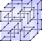
stacking of many metal layers. Hence, one can consider surrounding a security-sensitive cir-cuit part by a wire cage, for instance a Hamiltonian path connecting the vertices of a cube (Fig. 1). In this paper, different algorithms to construct cubical Hamiltonian structures are studied; those ideas can be extended to other forms of sufficiently dense lattices.
Since 3D integration is based on the vertical stacking of different dies, a Hamiltonian cage can surround the whole target and protect its content from physical attacks. 3D ICs are rel-atively hard to probe due to the tight bonding between layers [11]. Moreover, the 3D path can even penetrate the protected circuit and connect points in space between the protected circuit’s transistors.
Fig. 1: Hamiltonian cycle passing through the vertices of a4×4×4cube
1A Hamiltonian circuit (hereafter ”cage” or simply ”path” for the sake of conciseness) is an
A path running through different metal layers and different dies can thus serve as adigital
integrity verification sensor allowing the sending and the collecting of signals. In addition, the wire can be used to fill gaps in empty circuit parts to increase design compactness and make reverse-engineering harder.
Such a protection proves challenging in terms of design as it requires devising new manufac-turing and synthesis tools to fit the technology used [1,2]. However the resulting structures prove very helpful in protecting against active probing (cf.Appendix A).
Throughout this papernwill represent the number of points forming the edge of a cubi-cal Hamiltonian structure. We will focus our study on cubicubi-cal structures, but the algorithms and concepts that are presented hereafter can in principle be extended to many types of sufficiently dense lattices of points.
2
Generating Random 3D Hamiltonian Paths
2.1 General Considerations
The problem of finding a Hamiltonian path in arbitrary graphs (HAMPATH) is NP-complete. Membership in NP is easy to see (given a candidate solution, the solution’s correctness can be verified in quasi-linear time). We refer the reader to [3] for more information on HAM
-PATH.
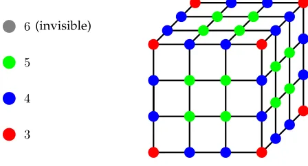
A quick glance reveals that a cube’sn3vertices, potentially connectable by a mesh of3n2(n− 1)edges, break-down into four categories, illustrated in Fig. 22:
– (n−2)3vertices corresponding to the cube’s innermost edges (i.e.not facing the outside) can be potentially connected in any of the possible 3D directions (right, left, up, down, front, rear).
– 6(n−2)2 vertices, facing the cube’s outside in exactly one direction, can be potentially connected in five possible directions.
– 12(n−2)vertices, facing the cube’s outside in exactly two directions, can be potentially connected in four possible directions.
– 8 extreme corner vertices can be connected in only three possible manners.
Indeed:(n−2)3+ 6(n−2)2+ 12(n−2) + 8 = ((n−2) + 2)3=n3
3 4 5
6(invisible)
Fig. 2: Potential edge connectivity
We observe that forHAMPATHto be solvable in a cube,nmust be even. If we depart from point the(0,0,0)and reach a point of coordinates(x, y, z)after visitingivertices, thenx+
y+zandihave the same parity. Given that the path must collect all the cube’s vertices, the cube size must necessarily be even.
2.2 Odd Size Cubes
The above observation excludes the existence of odd-size cubes unless one skips in such cubes an edge(x, y, z)such that x+y+z ≡ 1 mod 2. To extend the construction to odd
n = 2k+ 1while preserving symmetry, wearbitrarilydecide to exclude the central vertex (i.e.at coordinate(k, k, k)) whennis odd.
Assume that we color vertices in black and white alternatingly (the cube’s 8 extreme vertices being black) with black corresponding to even-parityx+y+zand white corresponding to odd parityx+y+z. Here0≤x, y, z≤2k. In other words, a(2k+ 1)-cube has4k3+ 6k2+ 3k white vertices and4k3+ 6k2+ 3k+ 1black vertices.
The coordinate of the cube’s central vertex is(k, k, k)which parity is identical to the parity ofk. Whenkis even, vertex(k, k, k)is black and whenkis odd vertex(k, k, k)is white. If we remove vertex(k, k, k)it appears that:
– When kis even, (i.e.n = 2k+ 1 = 4`+ 1) we have as many black and white vertices (namely4k3+ 6k2+ 3k).
– Whenkis odd, we have4k3+ 6k2+ 3k+ 1black vertices and4k3+ 6k2+ 3k−1white vertices.
Noting that each edge causes a color switch, we see that Hamiltonian paths in cubes of size 4`+3cannot exist. Note that if one extra black vertex is removed3then (the now asymmetric)
construction becomes possible for allk.
It remains to prove that cubes of sizen= 4`+ 1exist for all`6= 0 . This is seen to be true given the extensible structure shown in Appendix B. If`is increased, the structure can be re-scaled by enlarging each floor by four units and piling up four additional floors (two at the top and two at the bottom).
As a purely theoretical side-note, although we have not fully analyzed the constructibility problem in higher dimensions, it seems that 4D cubes of all sizes are ”constructible”. A hypercube of dimensiondhasnd vertices with a central vertex at coordinate(dk, . . . , dk). Hence whendis even the parity issueseemsto vanish.
3
A Toolbox for Generating 3D Hamiltonian Cycles
3.1 From Two to Three Dimensions
We start by presenting a first algorithm for constructing random4 Hamiltonian cycles in
graphs having a minimum degree equal to at least half the number of their vertices.
Our application requires an efficient algorithm that outputs cycles passing through a very large number of vertices. The first algorithm reduces the problem’s complexity by using smaller cycles that we will progressively merge to form the final bigger cycle. Consider the elementary Hamiltonian cycle forming a simple2×2square. To combine two such squares all we need are two parallel edges. Merging (denoted by the operator!) can be done in two ways as shown Fig. 3. Note that this association not only preserves Hamiltonicity but also extends it.
a b → a!b
a b
→
a
!
b
Fig. 3: Association of squares along thexaxis (leftmost figure), or theyaxis (rightmost figure)
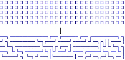
In other words, at each step two different Hamiltonian cycles in adjacent graphs are merged, and a new Hamiltonian cycle is created. The process is repeated until only one Hamiltonian cycle remains. We implemented this process in C. As explained previously, our program cannot find Hamiltonian cycles for odd cardinality values simply because such cycles do not exist (see Algorithm 1). The code starts by filling the lattice with 2×2squares, and then associates them randomly. The program ends when only one cycle is left (Fig. 4).
Fig. 4: Rewriting 125 squares filling a50×10lattice as a Hamiltonian cycle using Algorithm 1
Algorithm 1Cycle Merging
1: Inputp, q∈2N.
2: letQ=Q1, ..., Qvbe thev= pq4 squares of size 2 filling the lattice ofp×qpoints.
3: while Card(Q)6= 1do
4: choose randomly{a, b} ∈Q2witha6=b.
5: ifaandbhave at least one couple of neighbouring parallel edgesthen
6: Break a randomly chosen couple of parallel neighbouring edges, verify that they form a single Hamiltonian circuit and mergec=a!b.
7: letQ=Q∪ {c} − {a, b} 8: else
9: gotoline 4
10: end if
11: end while
4As explained in Appendix C , the entropy of our structure generators seems very complex to
The algorithm is pretty fast, and we were able to build Hamiltonian cycles of105 points using a laptop5 within few seconds. For somepandqvalues, we observed some runtime
spikes in single measurements due to convergence issues. Fig. 5 shows the average runtime over 100 measurements as well as the standard deviation at each point in red.
5 15
0 15 30 45 60 75 90
T
ime
(s)
Fig. 5: Cycle Merging runtime as a function of the number of points×103(average over 100
measurements)
To transform a rectangular 2D Hamiltonian cycle into a 3D one, we run Algorithm 1 for {p, q}={p, p2}to get ap×p2rectangleLsimilar in nature to the one shown in Fig. 4.
Then, letting(xi, yi)denote the Cartesian coordinates of points inL, with the first point being (0,0), we foldLinto a 3D structure of coordinates(xi0, y0i, zi0)using the following transform wherej=bxi
pcand`≡jmod 2:
ϕ=
x0i= (−1)`(xi−jp) +`(p−1)
yi0=yi
zi0=j
The result is shown in Fig. 26 (Appendix D).
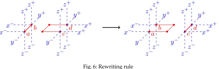
It remains to destroy the folded nature of the construction while preserving Hamiltonicity. This is done as follow: Identify anywhere in the generated structure the red pattern shown at the leftmost part of Fig. 6 where at positionsa, b, c, dedges take any of the blue positions. Iteratively apply this rewriting rulealong any desired axisuntil the resulting structure gets ”mixed enough” to the designer’s taste. Evidently, this is only one possible rewriting rule amongst several.
b
a
x
−x
−z
−z
−z
+z
+y
+y
−d
c
x
+x
+z
−z
−z
+z
+y
+y
−b
a
x
−x
−z
−z
−z
+z
+y
+y
−d
c
x
+x
+z
−z
−z
+z
+y
+y
−Fig. 6: Rewriting rule
Note that the zig-zag foldingϕis only one among many possible folding options asϕmay be replaced by any 2D (preferably random) plane-filling curve of size p×p(e.g. a Peano curve [8]).
3.2 Random Cube Association
Another approach consists in generalizing Algorithm 1 to the associating of elementary 3D cubes. As shown in Fig. 28, one can fill the target lattice by a random sampling of six ele-mentary Hamiltonian cubes (Fig. 27), associate them randomly and further randomize the resulting structure by rewriting.
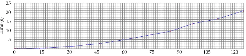
The algorithm proves very efficient (Fig. 7) and takes a few seconds6to compute a random
Hamiltonian cube of size 50 (125 000 points).
5 10 15 20 25
0 15 30 45 60 75 90 105 120
T
ime
(s)
Fig. 7: Random Cube Association runtime as a function of the number of points×103(average over
100 measurements)
The algorithm picks random parallel edges from different Hamiltonian cycles and attempts to associate them in one new structure. By opposition of the 2D case, the 3D case presents a new difficulty which is that in some cases associable parallel edges suddenly cease to exist. To force termination we abort and restart from scratch if the number of iterations executed without finding a new association exceeds the upper boundp3. To compute structures over huge lattices (e.g.n = 100), one might need to introduce additional association rules (e.g.
the rule shown in Fig. 8) to avoid such deadlocks.
!
Fig. 8: An additional association rule (example)
3.3 Cycle Stretching
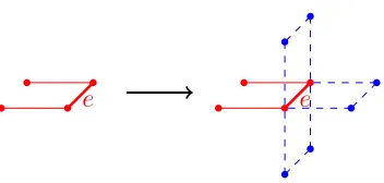
Our third algorithm maintains and extends a set of edgesEinitialized with the four edges defined by the square of vertices(0,0,0),(0,1,0),(1,1,0)and(1,0,0). At each iteration, the algorithm selects a random edgee∈ E and one of the four extension directions shown in Fig. 9. If such an extension is possible (in other words, by doing so we do not bump into an edge already inE) thenEis extended by replacingeby three new edges (one parallel toe
and two orthogonal toein the chosen extension direction). Ifecannot be replaced,i.e.none of the four extensions is possible, we pick a newe0∈Eand try again.
e
e
Fig. 9: Extension options
The algorithm keeps track of a subset ofE, denotedB, interpreted as the set of potentially stretchable edges ofE.Bavoids trying to stretch the sameeover and over again.
At each stretching attempt the algorithm picks a randome ∈ B. As the algorithm tries to stretche,eis removed fromB (no matter if the stretching attempt is successful or not). If stretching succeeded,eis also removed fromEand three new edges replacingeare added toBandE.
The algorithm halts whenB =∅. If upon halting|E|=n3−(nmod 2)then the algorithm
succeeds, otherwise the algorithm fails and has to be re-launched. Since at most3n2(n−1) vertices can be added toB, the algorithm will eventually halt.
A non-optimized implementation running on a typicalPCfound a solution forn= 6in about a minute and a solution forn= 8in 30 hours. The same code was unable to find a solution for n = 10 in three weeks. An empirical human inspection of the obtained cubes shows that the resulting structures seem very irregular. Hence, an interesting strategy consists in generating a core cube of sizen= 8by cycle stretching, surrounding it by elementary size 2 cubes and proceeding by random cube association and rewriting.
Algorithm 2Edge Stretching
1: letE=the four vertices defined by the square(0,0,0),(0,1,0),(1,1,0),(1,0,0). 2: letB=E.
3: whileB6=∅do
4: lete∈RB, we denote the vertices ofebye= [e1, e2].
5: letB=B− {e}
6: letdir={←,→,↑,↓,%,.}
7: whiledir6=∅do
8: letd∈Rdir 9: letdir=dir− {d}
10: ifdandeare not aligned and stretching is possiblethen
11: E=E− {e}.
12: E=E ∪ {[e1, v1],[v1, v2],[v2, e2]}.
13: break
14: end if
15: end while
16: end while
In the above algorithm the sentence ”stretching is possible” is formally defined as the fact that no edges inEpass through the two verticesv1,v2such that the segment[v1, v2]is parallel toein directiond. Arrows represent right, left, up, down, front and backwards directions,
3.4 Constraining Existing Hamiltonian Pathfinding Algorithms
A fourth experimented approach consisted in adapting existingHAMPATHsolving strategies. (Dharwadker) [4] presents a polynomial time algorithm for finding Hamiltonian paths in certain classes of graphs. Assuming that the graphs that we are interested in are in such a class, we tweaked [4]’s C++ code to find Hamiltonian cycles in cubes. The resulting code succeeded in finding solutions, but these had a too regular appearance and had to be post-processed by re-writing.
We hence constrained the algorithm by working in a randomly chosen subgraphE of the fulln3cube. We define adensity factorγ ≤1allowing to control the number of edges inE to which we apply [4]. The ratio of edges inEandn3is expected to be approximatelyγ. Note that because of the heuristic corrective step (9), meant to reduce the odds that certain points remain unreachable,E’s density is expected to be slightly higher thanγ. The corresponding algorithm is:
Algorithm 3Edges Selection Routine 1: E=∅
2: foreach vertexv= (x, y, z)of the full cubedo
3: foreach move dv= (dx,dy,dz)in{(1,0,0),(0,1,0),(0,0,1)}do
4: generatea randomr∈[0,1]
5: ifr < γand(0,0,0)≤v+dv≤(n−1, n−1, n−1)then
6: addedge[v, v+dv]toE
7: end if
8: end for
9: ifloop 3 didn’t add toEany edge havingvas en extremitythen
10: gotoline 3
11: end if
12: end for
Practical experiments show indeed that asγdiminishes, the generated Hamiltonian cycles seem increasingly irregular (for high (i.e.'1)γvalues the algorithm fills the cube by succes-sive ”slices”). Finding solutions becomes computationally harder asγdiminishes, but using a standardPC, it takes about a second to generate an instance for{γ = 0.8, n = 6}and an hour to generate a{γ = 0.86, n= 10}one. The reader is referred to Appendix F for several experimental results.
3.5 Branch-and-Bound
Another experimented approach was the use of branch-and-bound: Using a recursive func-tion, we can try all different cycles. Given a connected portion of a potential Hamiltonian path, this function tries to add all the possible new edges and calls itself recursively. If the function is called with a complete path, the job is done.
We added several heuristic improvements to this method:
1. If the set of vertices unlinked by the current path is disconnected, it is clear that we won’t be able to find any Hamiltonian path, and thus we can stop searching.
2. If this set is not connected to the extremities of the current path, we can also halt.
3. The existence of an Hamiltonian path containing a given sub-path only depends on the extremities and on the set of vertices in the path. We can hence use a dynamic program-ming approach to avoid redundant computations.
4. We tried multiple heuristics to chose the order of recursive calls.
However, those approaches proved much slower than cycle stretching: it appears that the branch-and-bound algorithm makes decisive choices at the beginning of the path without being able to re-consider them quickly. We tried to count all the Hamiltonian cycles when
n= 4using this algorithm, but the code proved too slow to complete this task in a reasonable time.
Those results suggest a meta-heuristic approach that would be intermediate between branch-and-bound and stretching: we can make a cycle evolve using meta-heuristics until we obtain an Hamiltonian cycle. Using this method (that we did not implement) we should be able to re-consider any previous choice without restarting the search process.
3.6 Rewriting 3D Moore Curves
Finally, one can depart from a know regular 3D cycle (e.g.a 3D Moore curve as shown in Fig.11) and rewrite it. Moore curves are particularly adapted to such a strategy given that the maze entrance and exit are two adjacent edges. However, as shown in Fig.11c (a top-down view of Fig.11b), Moore curves are inherently regular and must be re-rewritten to gain randomness.
(a) (b) (c)
4
Silicon Experiments
To test manufacturability in silicon we created a first passive cage meant to protect an 8-bit register. We notice that the compactness of the cage provides a very good reverse-engineering protection.
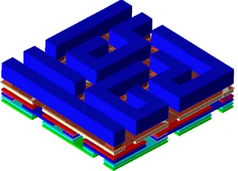
Fig. 12: 3D layout of a cage of size 6 (130nm, 6 Metal Layers Technology)
The implemented structure (Fig. 12) is a6×6×6Hamiltonian cube stretching over six metal layers, the first four metal layers are copper ones, and the last two metal layers are thicker and made of aluminum (130nm RF technology, Fig. 13). The cube is 26µm wide and covers an 8 bit register.
As will be explained in the next section, this first prototype is not dynamic, the Hamiltonian path is not connected to transistors. The implementation of a simplified dynamic structure as described in section 5 is underway and does not seem to pose insurmountable technological challenges. Moreover, all layers of the prototype are processed in one side of the silicon, so this implementation does not prevent backside attack. Backside metal deposit and back to back wafer stacking must thus be investigated to thwart backside attacks as well.
(a) (b)
Fig. 13: Top layer view (a) and tilted SEM view (b) of a 26µm wide6×6×6cage implemented in a 130nm technology (×2500)7
7The structure implemented in silicon is surrounded by fill shapes used as a gaps filler, due to
5
Dynamically Reconfigurable 3D Hamiltonian Paths
A canary is a binary constant placed between a buffer and stack data to detect buffer over-flows. Upon buffer overflow, the canary gets corrupted and an overflow exception is thrown. The term ”canary” is inherited from the historic practice of using canaries in coal mines as toxic gas biological alarms. The dynamic structures presented in this section are hardware equivalents of biologic canaries: our ”hardware canary” is formed of a spatially distributed chain of functionsFipositioned at the vertices of a 3D cage surrounding a protected circuit. In essence, a correct answer(Fn ◦. . .◦F1)(m)to a challengemwill attest the canary’s in-tegrity. The device described in this section relies on a library of paths precomputed using the toolbox of algorithms described in the previous section.
5.1 Reconfigurable 3D Mazes
The construction of a 3D dynamic grid begins with the description of a Network On Silicon (NOS) with speed, power and cost constraints [7,12]. As described in [6,9], metal wires are shared, or made programmable, by introducingswitch-boxes, that serve as the skeleton of the dynamic Hamiltonian path. Each switch-box is an independent cryptographic cell that corresponds to a vertex of the graph. The switch-boxes are reconfigurable and receive recon-figuration information as messages flow through the Hamiltonian path during each session
c. All boxes are clocked8, and able to perform basic cryptographic operations. Six cell-level
parameters are used to define each switch-box:
– Acoordinate identifieriis a positive integer representing the ordinal number of the box’s Cartesians coordinates:i.e.i=x+ny+n2z.
– A session identifier c is an integer representing the box’s configuration: this value is incremented at each new reconfiguration session.
– Akeykishared with the protected processor located inside the cage.
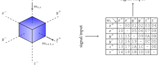
– Arouting configurationwi,cchosen between the thirty possible routing positions of a 3D bi-directional switch (Fig. 14)9.
– Astate variablesi,ccomputed at each clock cycle from the incoming datami,c(see here-after) and the preceding state,si,c−1. The statesi,cis stored in the switch-box’s internal
memory10.
mi+1,c=F(mi,c, ki, wi,c, si,c)
si,c+1=G(mi,c, ki, wi,c, si,c) (1)
The output datami+1,cis computed within boxiusing the input datami,cand an integrated cryptographic functionF, serving as a lightweight MAC. The final outputmn3,cattests the
cage’s integrity during sessionc.
z+ x− y− z− x+ y+ mi,c mi+1,c
wi&x+x−y+y−z+z−
x+ - 00 01 02 03 04
x− 10 - 05 06 07 08
y+
11 15 - 09 0A 0B
y− 12 16 19 - 0C 0D
z+
13 17 1A 1C - 0E
z− 14 18 1B 1D 1E
-signal output
signal
input
Fig. 14: Example of a 3D switch-box programmed with a routing configurationwi=0x13
8We denote bytthe clock counter.
9For switch-boxes depicted in red, blue and green (Fig. 2) the number of possible configurations
drops to (respectively) 6, 12 and 20.
10Upon resetsi,
Each switch-box comprises five logic parts (Fig. 15) that serve to route the integrity attesta-tion signal through the box’s six IOs and successively MAC the input valuesmi,c:
– Two multiplexers routing IOs, with three state output buffers to avoid short-circuits dur-ing re-configuration.
– A controller commanding the two multiplexers’ configuration.
– A MAC cell for processing data and a register for storing results.
– A register storing the state variablesi,c, the keyki, the present configuration wi,c, the next box configurationwi,c+1and the clock countert.
input pins
6 to 1
Multiplexer Controller
CLK
MAC and registry
CLK
1 to 6 Multiplexer with three-state buffers
output pins
z− z+
y− y+
x− x+
z− z+
y− y+
x− x+
Fig. 15: Logic diagram of a 3D switch-box
The input messagem0,c, sent through the Hamiltonian path, is composed of two parts serv-ing different goals (Fig. 16):
w0,c+1 w1,c+1 wi,c+1 wn3−1,c+1 cryptographic payload
reconfiguration information
Fig. 16: Structure of messagem0,c
– The first message part is dedicated to reconfiguring the grid. For a cube of sizen, the reconfiguration information hasn3parts, each containing the next routing configuration
wi,c+1 of switch-boxi. As the routing information of each switch-box can be coded on 5 bits, the reconfiguration information is initially5n3bits long11. Basically, this message
part carries the position of all switches for the next Hamiltonian path of sessionc+ 1.
– The second message part (cryptographic payload) is used to attest the circuit’s integrity, the 64-bits payload will be successively MACed by all switch-boxes and eventually com-pared to a digest computed by the protected circuit. If possible, one should select a func-tionF that simplifies after being composed with itself to reduce the protected circuit’s computational burden.
5.2 Description of the Dynamic Grid and the Integrity Verification Scheme
Upon reset, each switch-box is in a default configuration wi,0 corresponding to an initial predefined hardwired Hamiltonian path for sessionc = 0. The input and the output boxes (S0 andSn3−1) are only partially reconfigurable; namely, the routing ofS0’s input and the routing ofSn3−1’s output cannot be changed. To clarify the reconfiguration dynamics, we
denote bytthe number of clock ticks elapsed since system reset assuming a one bit per clock tick throughput; given that 5 bits are dropped at each ”station”, a full reconfiguration route (session) claims
5 n3−1
X j=0
(n3−j) = 5 2n
3(n3+ 1)
clock ticks, which is the time needed for the reconfiguration information to flow through all
n3 switch-boxesi.e.the number of clock ticks elapsed between the entry of the first bit of
m0,c intoS0and the exit of the last bit ofmn3,c fromSn3−1. Note that this figure does not
account for the time necessary for payload transit12.
Att= 0: A new sessioncstarts and the first bit ofm0,cis received byS0form the protected processor.
For5Pi−1 j=0(n
3−j) =5 2i(2n
3+ 1−i)≤t≤5Pi j=0(n
3−j)−1 = 5
2(i+ 1)(2n
3−i)−1: All switch-boxes exceptSi−1andSiare inactive (dormant).Si−1sends the messagemi−1,c toSiwhich performs the following operations:
– Store the reconfiguration informationwi,c+1, for the next Hamiltonian route of ses-sionc+ 1.
– Computemi+1,cand updatesi,c+1as defined in formula (1). Att= 5Pn3−1
j=0 (n
3−j) =5 2n
3(n3+ 1): The first bit of messagem
n3,cemerges from the grid (fromSn3−1) and all switch-boxes re-configure themselves to the new Hamiltonian path
c+ 1.mn3,cis received by the protected processor who compares it to a value computed
by its own means. At the next clock tick a new messagem0,c+1is sent in, and the process starts all over again for a new route representing session numberc+ 1.
Switch-Box 0
(w0, k0, m0, s0)
Switch-Box 1
(w1, k1, m1, s1)
Switch-Box 2
(w2, k2, m2, s2)
Switch-Box 3
(w3, k3, m3, s3)
Switch-Box 4
(w4, k4, m4, s4)
Switch-Box 5
(w5, k5, m5, s5)
Switch-Box 6
(w6, k6, m6, s6)
Switch-Box 7
(w7, k7, m7, s7)
Switch-Box 8
(w8, k8, m8, s8)
Switch-Box 9
(w9, k9, m9, s9)
Switch-Box 10
(w10, k10, m10, s10)
Switch-Box 11
(w11, k11, m11, s11)
Switch-Box 12
(w12, k12, m12, s12)
Switch-Box 13
(w13, k13, m13, s13)
Switch-Box 14
(w14, k14, m14, s14)
Switch-Box 15
(w15, k15, m15, s15)
m0,c
m0,c+1
m16,c
m16,c+1
at sessionc
at sessionc+ 1
Fig. 17:4×4dynamic switch-box grid routed atcandc+ 1(illustration)
12p(n3
If one of the switch-boxes is compromised then the digest output by the path will be altered with high probability and the fault will be detected by the mirror verification routine imple-mented in the protected processor (Fig. 18). The device could then revert to a safe mode, and sanitize sensitive data.
challenge m0,c
MAC using the Hamiltonian circuit
MAC using the co-processor
if 1 then revert to safe mode
Fig. 18: Device integrity verification scheme
The verification circuit’s size essentially depends on the MAC’s size and complexity. Note that the XOR gate is a weak point: if it is bypassed the entire canary becomes pointless. Luckily, the XOR is spatially protected by the Hamiltonian path that surrounds it.
5.3 Vulnerability to Focused Ion Beam (FIB) Attacks
The proposed dynamic structure complies with the Read-Proof Hardware requirements de-scribed in [10]: the structure is easy to evaluate, relatively cheap (in some case no additional masks would be required) and can’t be easily removed without damaging the chip.
Even though an attacker might modify some switch-box interconnections using FIB equip-ment, one cannot bypass a switch-box without modifying the digest computation logic and thus triggering the canary. In theory, an attacker may microprobe the input of the first switch-box to get the reconfiguration path, feed it into an FPGA simulating the grid and re-feed the MAC into the target, thus bypassing the canary. The state functionsiimplemented in each box should prevent such attacks by keeping state information. Moreover, switch-boxes are defined at transistor level (first metal level): to microprobe each cell the attacker has to bypass many interconnections, making such an attack very complex. Fig. 19 describes schematically the dynamic grid concept.
S1 S2 S3
Fig. 19: Three switch-boxes embedded at substrate level with interconnections over the top layers
6
Perspectives and Open Problems
Hardware canaries present an advantage with respect to analog integrity protection such as PUFs and sensors: being purely digital, hardware canaries can be integrated at the HDL-level design phase be portable across technologies. The proposed solution would, indeed, increase manufacturing and testing complexity but, being purely digital, would also increase relia-bility in unstable physical conditions, a common problem encountered when implementing analog sensors and PUFs.
The previous sections raise several sophistication ideas. For instance, instead of having the processor simply pick a reconfiguration route in a pre-stored table, the processor mayalso re-writethe chosen route before configuring the canary with it. Devising more rewriting rules and developing lightweight heuristics to efficiently identify where to apply such rules is an interesting research direction.
Another interesting generalization is the interleaving in space of several disjoint Hamilto-nian circuits. Interleaved canaries will force the attacker to overcome several spatial barriers. It is always possible to interleave a cube of sizen−1in a cube of sizenwithout having the two cubes intersect each other13as illustrated in Fig. 20.
Fig. 20: A size 4 cube interleaved with a size 3 cube (3D and front view)
Fig. 21 shows the result of such a (laborious!) physical interleaving for a cube of size 4 and a cube of size 5. Note that interleaving remains compatible with a dynamic evolution ofboth cubesas canaries do not touch each other nor share any hardware (edges or vertices).
Fig. 21: Interleaving a Hamiltonian cube of size 4 and a Hamiltonian cube of size 5
Finally, functionsFfor which the evaluation ofF(x) = (Fn3−1◦. . .◦F0)(x)is faster thann3
individual evaluations ofFiare desirable for efficiency reasons. XOR, bit permutation, ad-dition, multiplication and exponentiation (e.g.modulo 251) all fall into this category14. Note thatFi(x) =ki×xk
0
i modpworks as well.
In the first dynamic prototype theFi’s will be formed of XORs and bit permutations. De-vising computational shortcuts taking into account an evolving internal statesi,c are also desirable.
13Remove the(k, k, k)point from the center of the odd cube as explained before.
A
Chip Probing
An optical probing station (Fig. 22) allow an attacker to feed and collect signals from a target chip through its input and output pins.
(a) (b)
Fig. 22: A decapsulated chip with an exposed pad ring (a) and an optical probing station (b).
To probe directly metal lines (Fig. 23b), an attacker must use more sophisticated tools. Using a probing station installed in a SEM (Fig. 23a), it is possible to probe apparent metal lines. To probe hidden metal lines, a FIB must be used to remove layers and create new connections.
(a) (b)
B
Constructing Cubes of Size
n
= 4
`
+ 1
Fig. 24: Constructive proof that cubes of sizen= 4`+ 1exist for all`6= 0
C
The Entropy of a Random Hamiltonian Path
The entropy of a random Hamiltonian path generatorG(n)for cubes of sizenis simply:
H(G(n)) =− un
X i=1
pilog2(pi)
Whereun denotes the number of distinct paths constructible within a cube of sizen and
D
Circuit Folding
Fig. 25:10×100Hamiltonian rectangleLprepared to be folded
Fig. 26:10×10×10Hamiltonian cubeϕ(L)obtained by folding Fig. 25
E
Random Cube Association
Five elementary cubes in Fig. 28 are shown in red to underline that all cubes forming Fig. 28 are still disjoint.
Fig. 27: The six elementary Hamiltonian cubes of size 2
Fig. 29: Ann= 10Hamiltonian path obtained by randomly associating Fig. 28
F
Constrained Execution for Several
γ
Values
γ= 1.00 γ= 0.95
γ= 0.90 γ= 0.85
Fig. 30: Structures obtained for severalγvalues.
G
Experimental Pre-Silicon Models
Having obtained several construction plans, we decided to try and construct concrete exam-ples using copper supplies before migrating to silicon. We used an industrial robot to cut 12mm∅copper segments of various sizes. A measurement of the dimensions of off-the-shelf
Fig. 31: Angle connector
G.1 Visualizing and Layering
Layering and visualizing the prototypes (and chip metal layers) was done using anad-hoc
software suite written in C and in Processing15. The software allows decomposing a 3D
struc-ture into layers and rotating it for inspection.
3 1 1 2
floor 0
floor 1
1
3 1
1 1
2
1 1
1 1
1 1
1 1
1
1
floor 2
floor 3
Fig. 32: Layering, visualizing and constructing the prototypes.
G.2 Assembly Options
Segments were assembled using several techniques ranging from soldering to super-glue. The disadvantage of welding was the risk of unsoldering an angle connector while solder-ing the nearby one (and this indeed happened at times). Super-glue happened to be less risky but called for dexterity as the glue would harden in a couple of seconds and thereby make any further correction impossible. All in all super-glue was preferred and allowed the generation of a variety of experimental pre-silicon cubes shown in Fig. 33. 3D printing using stereolitography or thermoplastic extrusion (fused deposition modeling) were considered as well.
Fig. 33: Experimental pre-silicon cubes
G.3 Angular Deviation Problems
When assembling a 3D cage with glue (or soldering) it is very easy to make mistakes that add-up. A small angular deviation in the assembly of an angle along thexaxis will mix with a small angular deviation along they axis and quickly result in a distorted cage. To avoid this, we assembled structures using a process that consists in slicing the generated structure along the three axes and identifying the longest planar (2D) parts in the target construction. Each planar part is laid on a table and is hence glued according to two axes only (i.e.with a lesser degree of freedom). This makes 2D angular errors avoidable (in theory) or at least much smaller (in practice). As the 2D parts are dry and ready, they are glued to each other to form the final cage. As it turns out, this indeed yields much straighter constructions.
References
[1] C. Ababei, Y. Feng, B. Goplen, H. Mogal, T. Zhang, K. Bazargan and S. Sapatnekar,Placement and Routing in 3D Integrated Circuits, IEEE Design and Test of Computers, 22(6), pp. 520-531, Nov/Dec 2005.
[2] A.J. Alexander, J.P. Cohoon, J.L. Colflesh, J. Karro, E. Peters and G. Robins,Placement and routing for three-dimensional FPGAs, Fourth Canadian Workshop on Field-Programmable Devices, pp. 11-18, May 1996.
[3] B. Bollob´as,Graph Theory: An Introductory Course, New York: Springer-Verlag, p. 12, 1979. [4] A. Dharwadker,The Hamiltonian Circuit Algorithm, Proceedings of the Institute of Mathematics,
p. 32, 2011.
[5] R. Dickau, Hilbert and Moore 3D Fractal Curves, The Wolfram Demonstrations Project, http://demonstrations.wolfram.com/HilbertAndMoore3DFractalCurves
[6] K. Goossens, J. van Meerbergen, A. Peeters and P. Wielage,Networks on Silicon: Combinig Best-Effort and Guaranteed Services, Proceedings of Design Automation and Test Conference (DATE), pp. 423-425, 2002.
[7] J. Kim, I. Verbauwhede and M.-C. F. Chang,Design of an Interconnect Architecture and Signaling Technology for Parallelism in Communication, IEEE Trans. VLSI Syst. 15(8), pp. 881-894, 2007. [8] E. H. Moore,On Certain Crinkly Curves, Trans. Amer. Math Soc., 1, pp. 72-90, 1900.
[9] E. Rijpkema, K. G. W. Goossens, A. Radulescu, J. Dielissen, J. van Meerbergen, P. Wielage, and E. Waterlander,Trade offs in the design of a router with both guaranteed and best-effort services for networks on chip, Proceedings of Design, Automation and Test Conference in Europe (DATE), pp. 350–355, March 2003.
[10] P. Tuyls, G. Schrijen, B. Skoric, J. van Geloven, N. Verhaegh, R. Wolters,Read-Proof Hardware from Protective Coatings, Cryptographic Hardware and Embedded Systems, CHES 2006, LNCS vol. 4249, pp. 369-383, Springer, 2006.
[11] J. Valamehr, T. Huffmire, C. Irvine, R. Kastner, C¸ . Koc¸, T. Levin, and T. Sherwood,A Qualitative security Analysis of a New Class of 3-D Integrated Crypto Co-processors. Festschrift Jean-Jacques Quisquater, LNCS vol. 6805, pp. 364-382, Springer, 2011.
![Fig. 10: A n = 10 Hamiltonian cycle obtained by a modified version of Dharwadker’s algorithm [4]](https://thumb-us.123doks.com/thumbv2/123dok_us/7889565.1309205/8.612.242.374.574.709/fig-hamiltonian-cycle-obtained-modied-version-dharwadker-algorithm.webp)
![Fig. 11: Example of Moore Curves [5]](https://thumb-us.123doks.com/thumbv2/123dok_us/7889565.1309205/9.612.112.508.525.670/fig-example-of-moore-curves.webp)