Load Flow Solution for Radial Networks with Composite and Exponential Loads

(1)

Load Flow Solution for Radial Networks with

Composite and Exponential Loads

Gowthami Kunche1, K. V. S. Ramachandra Murthy 2

M. Tech (PE), Aditya Engineering College, Surampalem, East Godavari District, Andhra Pradesh, India1 Professor, Aditya Engineering College, Surampalem, East Godavari District, Andhra Pradesh, India 2

ABSTRACT: A network-topology-based method is used to solve the load-flow problem of radial distribution networks in this Thesis. Power flow equations in matrix form are developed based on the topology. The technique requires line data in such way that the receiving end node must be in an ascending order. The implemented method requires building of two matrices: BIBC and branch-current to bus-voltage (BCBV) matrix. The bus-injection to branch-current (BIBC) is built by assigning unity to the nodes of the discovered paths. The method requires less number of iterations i.e., maximum of 3 iterations for convergence. In this Thesis, constant power load, constant current load, constant impedance load, composite and exponential loads have been considered for load flow solution. Load flow is obtained for 15 Bus, 33 Bus, 69 Bus and 85 Bus Systems. Load flow results are presented for various systems and also presented in graphical form. Results obtained for various types of loads are compared with the established results in the literature. They are found to be accurate to the third digit. Load flow algorithm is implemented in MATLAB.

KEYWORDS: Radial networks, Load flow, Bus system, Topology, MATLAB.

I.INTRODUCTION

Load flow analysis of distribution systems has not received much attention unlike load flow analysis of transmission systems. However, some work has been carried out on load flow analysis of a distribution network but the choice of a solution method for a practical system is often difficult. Generally distribution networks are radial and the

R/X ratio is very high. Because of this, distribution networks are ill-conditioned and conventional Newton-Raphson (NR) and fast decoupled load flow (FDLF) methods are inefficient at solving such networks. Many researchers have suggested modified versions of the conventional load flow methods for solving ill-conditioned power networks. Recently researchers have paid much attention obtaining the solution of distribution networks. In India, all the 11 kV rural distribution feeders are radial and too long. The voltages at the far end of many such feeders are very low with very high voltage regulation. In this project, the main aim has been to implement a load flow technique for radial distribution networks. This method involves construction of two network matrices based on topology and matrix operations. Computationally this method is very efficient. Another advantage of this method is that it requires less computer memory. Convergence is always guaranteed for any type of practical radial distribution network with a realistic R/X ratio while using this method. Loads, in the present formulation, have been represented as constant power. However, this method can easily include composite load modeling if the break up of the loads is known. This load flow technique has been implemented using MATLAB. Several practical rural radial distribution feeders in India have been successfully solved using this method. In this paper, only 10 bus unbalanced system is considered. Relative speed and memory requirements of this load flow method are better than method proposed by Baran and Wu as per the literature.

(2)

distribution level. in recent years, considerable attention has been focused in planning of a distribution system, to reduce the power and energy losses, to reduce the capital investment involved and to provide better quality supply to consumers. Improved modeling techniques and certain optimization and programming approaches have been presented to determine the best location, and suitable interconnections between sub-stations so as to meet the increasing demands more reliably and economically. In these approaches, shunt capacitors are introduced to reduce losses and to provide reactive power compensation. A Distribution system is one from which the power is distributed to various users through feeders, distributors and service mains. Feeders are conductors of large current carrying capacity, carrying the current in bulk to the feeding points. Distributors are conductors from which the current is taped off for supply to the consumer premises. The size of feeder is determined primarily by the currents it is required to carry, and on the other hand the permissible voltage along a distributor forms the main basis of design in case of a distributor. The size and cross-section, of feeders and distributors are affected by the increase in supply voltage. It has been established that 70% of the total system losses are occurring in the primary and secondary distribution system, while transmission and sub- transmission lines account for only 30% of the total losses. Therefore the primary and secondary distribution systems must be properly planned to ensure losses within the acceptable limits.

Distribution Automation Systems have evolved both in concept and implementation over a period of time. The distribution power flow has influenced other applications such as network optimization, VAR planning and switching. The distribution systems, characterized by their prevailing radial nature and high r/x ratio, render them to be ill-conditioned and make the traditional Newton-Raphson (NR) and fast decoupled power flow (FDPF) solution techniques unsuitable. Consequently many power flow algorithms specially suited for distribution systems have emerged and are well documented . These methods are roughly viewed as node based and branch based methods. The first category has used node voltages or current injections as state variables and requires information on the derivatives of network equations. Abul Wafa et al have used a graphical approach for developing loadflow equations in matrix form to satisfy the need of distribution automation. Depth first search is used to trace the path of power flow direction. Matrices are developed based on discovered path [1]. Teng and Lin developed topology based load flow solution [2]. A simple power flow method for radial distribution networks proposed by Das et al involves evaluation of simple algebraic expressions of the receiving-end voltages. No importance is given for initial guess solution in Das et al and other related research works [3]. Shirmohammadi et all have presented a compensation-based power flow method for weakly meshed distribution and transmission systems [4]. Stevens et al have shown that the ladder technique is found to be fastest but did not converge in five out of 12 cases studied [5]. Goswami and Basu have presented a direct solution method for solving radial and meshed distribution networks [6]. Jasmon and Lee have derived the fundamental equations for solving a load flow problem of a distribution network using a single-line equivalent [7]. Goswami and Ghosh have presented a direct method for solving radial and mesh distribution networks [8]. Haque has proposed a method suitable for both radial and mesh configurations. It being a Z-bus based method, the sparsity structure cannot be exploited which is the greatest disadvantage. Das et al have suggested a load flow solution for meshed distribution networks only. The meshed distribution network is converted into a radial network, by selecting break points. The branch current interrupted by the creation of every break point can be replaced by current injections at its two nodes without affecting the network operating conditions. Sparse methods cannot be applied being a Z-Bus based method [9].

II.TOPOLOGY BASED LOAD FLOW SOLUTION

Equivalent current injection: For distribution systems, the models which are based on the equivalent current injection as reported by Shirmohammadi et al., (1988), Chen et al. (1991.) and Teng and Lin (1994) are more convenient to use. At each bus ‘k the complex power Sk is specified by,

= P + j Q (1)

(3)

= + ( ) =

∗

(2) is the node voltage at the kth iteration.

is the equivalent current injection at the k-th iteration.

and are the real and imaginary parts of the equivalent current injection at the k-th iteration respectively.

Bus-Injection to Branch-Current matrix : ( BIBC)

The power injections can be converted into equivalent current injections using the equation(1). The set of equations can be written by applying Kirchoff’s current law ( KCL) to the distribution network. Then the branch currents can be formulated as a function of the equivalent current injections.

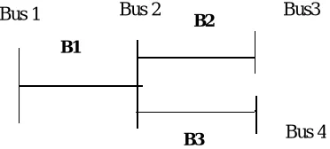
Fig. 1 Sample distribution system. B1= I3+ I4

B2=I3

B3=I4

Where, I2, I3 and I4 are load currents respectively at buses 2, 3 and 4

[B] = [BIBC] [I] (3)

=

1 1 1 0 1 0 0 0 1

The constant BIBC matrix has nozero entries of +1 only. For a distribution system with m-branch sections and n-buses, the dimension of the BIBC is m x (n-1).

Branch-Current to Bus-Voltage Matrix :

The relation between the branch currents and bus voltages can be obtained by following equations. V2 = V1 – B1 Z12

V3 = V2 - B2 Z23

where V2 , V3 are the voltages at node 2 and node 3. Z23 is the impedance between 2 and 3 nodes. The above

equations can also be written as ,

V1 – V2 =Z12 B1

V1-V3= Z12B1 + B2 Z23.

In general, [V1] - [Vk] = [Z] [ B] where Z matrix will have elements in the transposed matrix of BIBC matrix. V1

matrix contains all elements equal to 1.0pu.

[∆ ] = [ ][ ] (4)

That can be written as,

− = (5)

[∆ ] = [ ][ ][ ] (6)

That can be written as,

B1

B2

B3

Bus 1 Bus 2 Bus3

(4)

− =

1 1 1 0 1 0 0 0 1

(7)

2.1 Algorithm for Topology based Load Flow Method

1. Read the system data,

2. Build BIBC matrix as given in equation (3).

3. Transpose BIBC and multiply with impedances and obtain BCBV matrix as given in eq. (7).

4. Initialize iteration count =1. Calculate equivalent current injections using equation(2). Considering uniform voltage profile of 1 pu at all buses.

5. Obtain ∆V matrix using equation (4). 6. Obtain voltages at all nodes.

7. Calculate current injections using new set of voltages.

8. If the difference in currents between current iteration currents and previous iteration currents is greater than 0.001, then print the result, otherwise, increment of the count and repeat the procedure from step(4).

As already presented in the previous sections, two important steps involved in this algorithm are, [B] = [BIBC] [I] : matrix [I] is current injections. Branch currents expressed in terms of bus current injections.

[∆ ] = [ ][ ] : Voltage deviations expressed in terms of branch currents.

= + ( ) =

∗

Conversion of Power injections into current injections. From the above two

equations, [∆ ] = [ ][ ][ ]

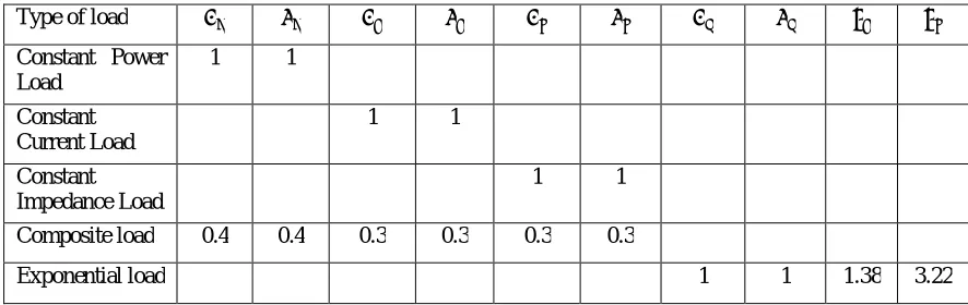
2.2 Load Modeling : The modeling of various types of loads are presented in this section. The general expression of load is shown below. The values of constants will be different for different loads.

= ( + + + )

Table 1 : Values of coefficients for different types of loads. Type of load

Constant Power Load

1 1 Constant

Current Load

1 1 Constant

Impedance Load

1 1 Composite load 0.4 0.4 0.3 0.3 0.3 0.3

Exponential load 1 1 1.38 3.22

2.3 Calculation of current for different types of loads :

Major part of the program is similar except that the calculation of current is different for different types of loads. It is described in this section.

For Constant Power load : currents=conj((p+q*i)./v);

(5)

For Constant Impedance load : currents=conj((p.*(v.^2)+q.*(v.^2)*i)./v);

For Composite load :

p=p.*(0.4+0.3*v+0.3*v.^2) q=q.*(0.4+0.3*v+0.3*v.^2) currents=conj(p+q*i./v);

For Exponential load : currents=conj((p.*(v.^1.38)+q.*(v.^3.22)*i)./v);

III.LOAD FLOW RESULTS FOR DIFFERENT TYPES OF LOADS

The load flow solution is obtained for constant power load, constant current load, constant impedance load, composite and exponential loads. For various types of loads, loadflow solution is obtained on 15 Bus, 33 Bus, 69 Bus and 85 Bus Systems. Sample program is presented in the Appendix 5. Data for the loadflow for 15 Bus, 33 Bus, 69 Bus and 85 Bus Systems is presented in Appendix 1 to Appendix 4 respectively. For 15 Bus system, 33 Bus system and 85 bus systems, the base voltage is 11 kV and base MVA is 100 MVA. For 69 bus system, base Voltage and base MVA are 12.66 kV and 100 MVA

Table 2 : Power Loss and Minimum voltage for 15-Node network Type of load Power loss Minimum

voltages(p.u) Real(KW) Reactive(KVAr)

CP 61.7803 57.30 0.9445 CI 56.142 52.05 0.9472 CZ 51.46 47.69 0.9496 Composite 56.73 50.31 0.9496 Exponential 50.26 46.59 0.9501

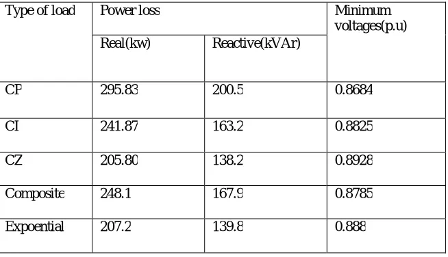
Table 3 : Power Loss and Minimum Voltage for 33-Node network Type of load Power loss Minimum

voltages(p.u) Real(kw) Reactive(kVAr)

(6)

voltages(p.u) Real(kw) Reactive(kVAr

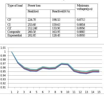
Fig.2 : Voltages on 15 Bus system

0.91 0.92 0.93 0.94 0.95 0.96 0.97 0.98 0.99 1 1.01

(7)

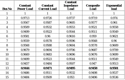
Table 6 : Voltages on 15 Bus System for various types of loads

Bus No

Constant Power Load

Constant Current Load

Constant Impedance

Load

Composite Load

Exponential load

1 1 1 1 1 1

2 0.9713 0.9726 0.9737 0.9719 0.974 3 0.9567 0.9587 0.9605 0.9577 0.961 4 0.9509 0.9532 0.9553 0.9521 0.9558 5 0.9499 0.9523 0.9544 0.9511 0.9549 6 0.9581 0.96 0.9616 0.959 0.9621 7 0.9559 0.9578 0.9596 0.9568 0.96 8 0.9568 0.9588 0.9604 0.9578 0.9609 9 0.9679 0.9694 0.9706 0.9687 0.9709 10 0.9669 0.9683 0.9696 0.9676 0.9699 11 0.9499 0.9523 0.9544 0.9511 0.9549 12 0.9457 0.9484 0.9507 0.947 0.9513

13 0.9444 0.9471 0.9495 0.9458 0.9501

14 0.9486 0.9511 0.9532 0.9498 0.9537 15 0.9484 0.9509 0.953 0.9496 0.9536

0.75 0.8 0.85 0.9 0.95 1 1.05

(8)

Table 7 : Voltages on 33 Bus System for various types of loads

Bus No Constant Power

Constant Current

Constant

Impedance Composite

Exponential load

1 1 1 1 1 1

2 0.996 0.9963 0.9965 0.996 0.9965 3 0.9952 0.9955 0.9958 0.9952 0.9957 4 0.9767 0.9786 0.98 0.9767 0.9799 5 0.9902 0.9906 0.9909 0.9902 0.9909 6 0.9664 0.9693 0.9715 0.9664 0.9713 7 0.9719 0.9739 0.9755 0.9719 0.9753 8 0.9892 0.9896 0.9899 0.9892 0.9899 9 0.9561 0.9601 0.9631 0.9561 0.9628 10 0.9627 0.9652 0.967 0.9627 0.9668 11 0.9883 0.9887 0.989 0.9883 0.9889 12 0.9314 0.938 0.9429 0.9314 0.9425

13 0.9581 0.9608 0.9628 0.9581 0.9625

(9)

IV.CONCLUSIONS

The load flow solution is obtained for constant power load, constant current load, constant impedance load, composite and exponential loads. For various types of loads, load flow solution is obtained on 15 Bus, 33 Bus, 69 Bus and 85 Bus Systems. The obtained results are in close agreement with the results obtained in literature.

It is observed that on all the bus systems, lowest minimum voltage is obtained for constant power loads. For constant power loads, on 15 Bus system, minimum voltage obtained is 0.9445 pu, on 33 Bus system minimum voltage is 0.8684 pu, on 69 Bus system minimum voltage is 0.9092 pu and on 85 bus system, minimum voltage for constant power load is 0.8713 pu.

0.8 0.85 0.9 0.95 1 1.05

1 4 7 1013161922252831343740434649525558616467707376798285

0.86 0.88 0.9 0.92 0.94 0.96 0.98 1 1.02

(10)

Better voltage is profile is observed with exponential loads on 15 bus and 85 bus systems. The minimum voltages on 15 bus system is 0.9501 pu and on 85 bus system is 0.8959 pu. On 33 bus and 69 bus systems, better voltage profile is observed with constant impedance loads. On 33 Bus system, minimum voltage is 0.8928 pu and on 69 bus system is 0.922 pu

REFERENCES

1. Ahmed R, Abul Wafa, “A Network Topology based Load Flow for Radial Distribution Networks with Composite and Exponential Load,

Electric Power Systems Research”, Vol. 91, 2012, Pp. 37-43

2. Jen-Hao Teng, “A Network- Topology based Three-Phase Load flow for Distribution systems”, Vol.24, No.4, 2000, Pp. 259-264.

3. D. Das, D.P. Kothari, A Kalam “Simple and effcient method for load flow Solution of radial distribution networks”., Electrical Power and Energy Systems, Butterworth, Heinmann Publications, Vol 17, No.5, pp335 – 346,1995.

4. Shirmohammadi D., H.W. Hong, A. Semlyen, and G.X. Luo 1988, “ A compensation based power flow method for weakly meshed distribution

and transmission netowkrs. IEEE Trnaas. On Power Systes, Vol 3, pp 753-762.

5. W. H. Kersting and D. L. Mendive, “An application of ladder network theory to the solution of three phase radial load flow problem”, Proceedings of IEEE PES Winter meeting, New York, January 1976, pp. A76 0448.

6. S. K. Goswami, S. K. Basu: ’Direct solution of distribution systems’, IEE Transactions on Generation, Transmission & Distribution, Vol. 138,

No. 1, 1991, pp. 78-88.

7. S. Ghosh and D. Das: ’Method for load flow solution of radial distribution networks’, IEE Proceedings Generation, Transmission and

Distribution, Vol. 146, No.6, November 1999, pp. 641-648.

8. S.Ghosh and D.Das: ’An approach for load flow solution of meshed distribution networks’, IE Journal-EL, pp. 66-70.

9. J.H. Teng, A novel and fast three-phase load flow for unbalanced radial distribution systems, IEEE Transaction on power systems 17 (4) (2002) 1238-1244.

10. K. V. S. Ramachandra Murthy, M. Ramalinga Raju, G.Govinda Rao, K.Narasimharao, Topology based approach for efficient load flow