Computing with Large Time Steps for Electromagnetic Wave
Propagation in Multilayered Homogeneous Media
Nikitabahen N. Makwana* and Avijit Chatterjee
Abstract—We present an extension of Large Time Step (LTS) method to electromagnetic wave propagation involving multilayered homogeneous media. The LTS method proposed by LeVeque is an extension of Godunov’s method for the numerical solution of hyperbolic conservation laws. In this method, very large time steps are allowed by an increase in the numerical domain of dependence compared to conventional explicit methods constrained by the Courant-Friedrichs-Lewy stability criteria. This can lead to additional complexities when being applied to multilayered homogeneous media due to presence of material interfaces. Appropriate treatment of material interface boundaries is proposed in the present work in the context of finite volume time-domain method with LTS. Numerical examples are presented involving solution of time-domain Maxwell’s equations in a layered dielectric medium using LTS approach.
1. INTRODUCTION
The classical LTS method was proposed by LeVeque [1] to speed up the solution of nonlinear hyperbolic conservation laws like the Euler equations in gas dynamics [2–4] and shallow water equations in fluid mechanics [5–9] when being solved in a Godunov based finite volume framework. The LTS approach assumes waves arising out of solving Riemann problems at cell interfaces in a Godunov method to behave linearly. This linear behaviour allows superposition of waves to be used to update downwind cell values. This results in the Courant-Friedrichs-Lewy (CFL) criterion restriction on the explicit time step due to numerical stability considerations being bypassed. The large value of time step Δt, due to CFL number (ν) 1 in LTS method, can considerably speed up numerical simulations involving hyperbolic waves even with the increased per-grid-point computational load due to inclusion of more Riemann waves for updating grid values. The time-domain Maxwell’s equations in finite difference time-domain (FDTD) or finite volume time-domain (FVTD) context can be computationally very expensive if the explicit time step Δtis small due to fine meshes resulting from point-per-wavelength (PPW) requirements.
The LTS method was extended to the solution of time-domain Maxwell’s equations, in free space in a FVTD framework in [10]. It was shown that Δt(andν) can be unconditionally large for 1D problems given that the time-domain Maxwell’s equations constitute a system of linear hyperbolic conservation laws. Fewer time steps in the LTS method also result in enhanced accuracy because of reduced discretization errors. Extension to multidimensions through operator splitting is also unconditionally stable using LTS, but the accuracy may degrade for ν 1. This is attributed to splitting error arising from the fact that Jacobian matrices in the multidimensional form of the time-domain Maxwell’s equations do not commute [11].
In the present work, we extend the LTS method in an FVTD framework to multilayered homogeneous media. We consider perfect dielectrics in a 1D domain. Dielectric slabs result in material interfaces which require special treatment in the LTS framework. Material interfaces can separate
Received 14 January 2019, Accepted 19 March 2019, Scheduled 3 April 2019 * Corresponding author: Nikitabahen N. Makwana ([email protected]).
material of constant or variable impedance. Propagating waves resulting from Riemann problem in the LTS method, encountering a constant impedance material interface, continue to update cells only in downwind direction of the interface. But the range of downwind cells is now dictated by the new wave speed downwind of the interface. Riemann waves encountering dielectric interface of variable impedance, on the other hand, produce reflected and transmitted waves at the interface. The amplitudes of the waves depend on reflection and transmission coefficients based on satisfying conservation at the material interface. Riemann waves encountering such an interface update both upwind and downwind cells to the interface. The range of cells, in both directions to be updated, depend on the local wave speed. Appropriate interface boundary conditions will form a part of the LTS framework involving layered media consisting of perfect dielectrics considered in this work. In a simple 1D domain Riemann waves, in-principle, can cross multiple dielectric interfaces in a single time step in an LTS method. This would be difficult to implement for practical problems in multidimension involving variable impedance media. The 1D problem solved here can also provide a condition for minimum thickness of dielectric slabs that can be efficiently solved using LTS for variable impedance media in more practical problems.
2. GOVERNING EQUATIONS
The time-domain Maxwell equations in differential form for a linear medium can be written as
∇ ×E = −∂B
∂t (1a)
∇ ×H = ∂D
∂t +J (1b)
where E is the electric field vector, H the magnetic field vector, D the electric flux density, B the magnetic flux density, and Jthe electric current density.
The constitutive relation for homogeneous and non-dispersive medium are given by
D = E=0rE, (2a)
B = μH=μ0μrH (2b)
where is the electric permittivity and μ the magnetic permeability of the medium. In Equation (2), 0= 8.854×10⁻¹² (farad/meter) andμ0= 4π×10−7(henrys/meter) are free space electric permittivity
and magnetic permeability, whiler and μr are relative permittivity and permeability of the medium. r= 1 andμr= 1 for free space. We initially present an overview of the LTS formulation for the solution of 1D Maxwell’s equations in homogeneous medium. This formulation is then extended to multilayered homogeneous media and numerical examples solved.
3. LTS METHOD IN HOMOGENEOUS MEDIUM
The source freex-directed andy-polarized 1D Maxwell’s equations are given by ∂Ey
∂t = − 1
∂Hz
∂x (3a)
∂Hz ∂t = −
1 μ
∂Ey
∂x (3b)
For the solution of Equation (3) using the LTS approach in an FVTD framework, the equations are written in conservative form as
∂u ∂t +A
∂u
∂x = 0 (4)
where conserved variableu and Jacobian matrix A=∂f(u)/∂x are given as
u=
Ey Hz
and A=
0 1/ 1/μ 0
The eigenvalues and eigenvectors matrix ofA are
Λ =
−c 0
0 c
and R=
−Z Z
1 1
(6)
where c = 1/√μ is the wave speed, and Z = μ/ is the impedance of the medium. In an FVTD framework [11], the spatial domain is subdivided into a number of finite volumes (cells), and over each cell the conservative form of Maxwell’s equations (4) is solved in an integral form. For a finite volume vi= [xi−1/2, xi+1/2], the integral form of Eq. (4) over a time interval tn to tn+1 can be written in a cell
centered discrete form as
Uni+1=Uni − Δt Δx
A+ΔUn
i−1/2+A−ΔUni+1/2
(7)
whereUni is the approximated cell average value ofuover the cell interval [xi−1/2, xi+1/2] at timetn, and
A±ΔUn
i∓1/2 is the numerical flux function at cell interfacexi∓1/2. A±can be defined as A±=RΛ±R− 1
where, Λ± = diag(λ±), and ΔUi−1/2 = Ui −Ui−1. λ+ = max(λ,0), λ− = min(λ,0) where λ are
the eigenvalues of the Jacobian matrix A as in Equation (6) and Λ = Λ++ Λ−. For the solution of Equation (7) using a wave propagation form of LeVeque’s LTS method, the variable Ui is updated at each time step by incorporating the solution of Riemann problem at each cell interface of the upwind grid cells [3, 12]. The waves arising out of a Riemann problem at an interfacexi−1/2 is written as [11]
Uni −Uni−1= m
p=1
αpi−1/2rp = m
p=1
Δupi−1/2 (8)
The 1D problem in Equation (3) has m= 2 with wave speeds (−c, c). αpi−1/2 are the scalar coefficient or amplitudes of eigenvectors rp, which represents the linear waves in the eigenvector expansion in Equation (8), and are expressed as
α1
i−1/2 =
−(Ey|i−Ey|i−1) +Z(Hz|i−Hz|i−1)
2Z (9a)
α2
i−1/2 =
(Ey|i−Ey|i−1) +Z(Hz|i−Hz|i−1)
2Z (9b)
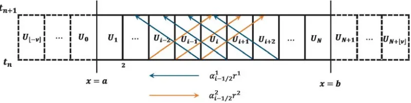
where Ey|i is the field Ey defined at the ith grid point. In homogeneous medium, the pth wave propagates with wave speedλp and propagates a distance|λp|Δtin each time step Δt. Thus, if the pth wave propagates an entire cell interval [xi−1/2, xi+1/2] the cell average gets incremented by a quantity αpi−1/2rp. If the wave traverses a part of the cell, a fraction ofαpi−1/2rp contributes to increment the cell average [3, 11, 12]. As shown in Figure 1, at each time step, thepth wave contributes to ν downwind grid cells by updating the cell averages, whereν=|λmax|Δt/Δxis the CFL number, andνmapsν to
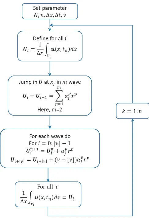
the least integer≥ν. λmaxis the maximum wave speed [12]. The classical LTS method due to LeVeque
is also shown in the form of a flowchart in Figure 2. In the flowchartν is the integer counterpart ofν.
Figure 2. LTS algorithm, homogeneous medium.
4. EXTENSION OF THE LTS METHOD TO MULTILAYERED HOMOGENEOUS MEDIA
For multilayered homogeneous media, the permittivity and permeability μare considered constant in a finite volume cell but can vary across cell faces. Equation (4) is now written as
∂u
∂t +A(x) ∂u
∂x = 0 (10)
where,
A(x) =
0 1/(x) 1/μ(x) 0
.
The eigenvalues and eigenvectors of Jacobian matrix A(x) are given by
Λ(x) =
−c(x) 0 0 c(x)
and R(x) =
−Z(x) Z(x)
1 1
(11)
where wave speedc(x) and impedanceZ(x) are defined as
c(x) = 1
μ(x)(x) and Z(x) =
μ(x)
(x). (12)
and impedance in each grid cell i are ci = 1/√μii and Zi = μi/i with i and μi the cell-wise values. For the conventional Godunov’s method (ν ≤1), a Riemann problem can straddle a material interface and influence evolution of the solution only in constituent cells containing that interface. The solution to the Riemann problem would then consist of single wave moving into either material for the 1D problem [11]. In the LTS framework multiple left and right moving waves can encounter a material interface. Interaction with the interface can create transmitted and reflected waves which will appropriately affect the domain traversed by the waves forν >1.
4.1. Constant Impedance Media
A special case of constant impedanceZ(x) =Z arises when the relation between μ(x) and (x) in the entire region of interest is μ(x) = Z2(x). In such cases, the eigenvectors rp(x) = rp are constant in space. Hence, waves in Riemann problems are defined identically as in Eq. (8) with the strength of the waves αpi−1/2 as in Eq. (9). The matrix of eigenvalues Λ(x) which represent wave speeds varies spatially withx for the multilayered homogeneous media. The wave speed in the Riemann problem at an arbitrary cell interfacexi−1/2 can be defined in an upwind sense asλ1i−1/2=−ci−1 andλ2i−1/2 = +ci.
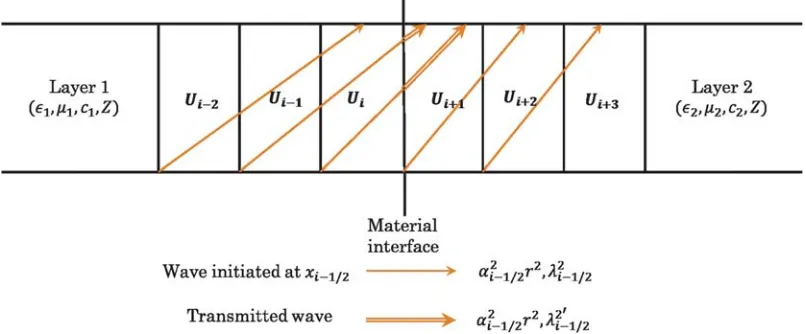
As shown in Figure 3, if thepth wave propagates entirely either in medium 1 or 2, with a wave speed λpi−1/2 in time Δt, then the wave propagates λip−1/2Δt distance and contributes toνi downwind grid cells to update cell averages, withνi defined as|λpi−1/2|Δt/Δx. On the other hand, if thepth wave with wave speed λpi−1/2 encounters a material interface after propagating k <νi downwind grid cells, the
wave transmits completely from one layer to another but with a change in wave speedλpi−1/2=ηλpi−1/2. For a right running wave (p = 2), η =μ11/μ22 is the refractive index between two layers. Due to
change in speed of wave to λpi−1/2, the wave propagates (k+η(νi−k))Δx distance and updates cell averages in a total ofk+η(νi−k)downwind cells instead ofνicells in time Δt(ν >1). In this case the entire wave is transmitted from one layer to another with compression/expansion of the original profile.
Figure 3. Right moving wave propagation in constantZ computational domain using LTS (schematic).
4.2. Variable Impedance Media
In the case of a change in impedance, along with the speed c(x), the eigenvector matrix R(x) suffers from a change across a material interface. The eigenvectors at an arbitrary cell interface xi−1/2 can again be defined as
r1
i−1/2=
−Zi−1
1
and ri2−1/2 =
Zi 1
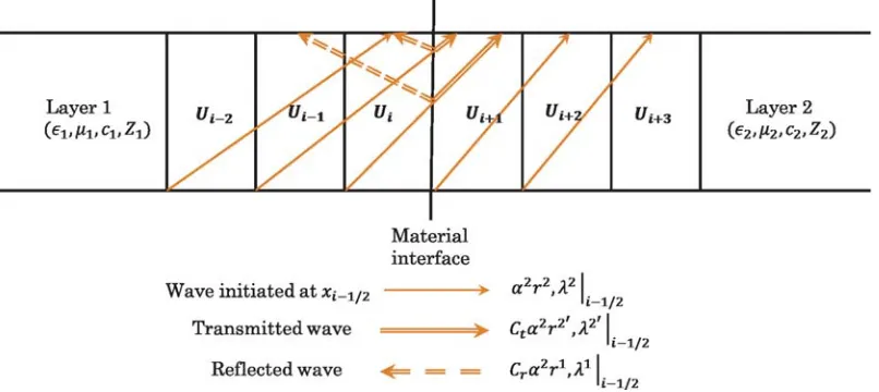
Figure 4. Right moving wave propagation in variableZ computational domain using LTS (schematic).
With these spatially varying eigenvectors rpi−1/2, local waves in each Riemann problem are defined as previously in Equation (8), and the strength of waves αpi−1/2 can be written as [11]
α1
i−1/2 =
−(Ey|i−Ey|i−1) +Zi(Hz|i−Hz|i−1)
Zi−1+Zi
(14a)
α2
i−1/2 =
(Ey|i−Ey|i−1) +Zi−1(Hz|i−Hz|i−1)
Zi−1+Zi .
(14b)
As shown in Figure 4, if thepth wave originating from the Riemann problem atxi−1/2 propagates
either entirely in medium 1 or 2, in time Δt with wave speed λpi−1/2, then the pth wave updates νi downwind grid cells withαpi−1/2rpi−1/2 as in homogeneous medium or constant impedance case. However, if thepth wave interacts with a material interface after propagatingk <νidownwind grid cells during time Δtonly a part of the incident wave is transmitted while the rest is reflected back from the material interface. This is in order to maintain conservation when a jump in impedance is encountered. The strength (amplitude) of transmitted and reflected wave are given byCtαpi−1/2andCrαpi−1/2, respectively. The transmission coefficient Ct and reflection coefficientCr for a right moving wave (p= 2) originating at an arbitrary interfacexi−1/2 and encountering a material interface of refractive indexη=μ11/μ22
are
Ct= ZZi−1+Zi i−1+ηZi
and Cr = ηZi−Zi Zi−1+ηZi.
(15)
For right moving waves (p = 2), the transmitted wave propagates η(νi −k)Δx distance and updates
η(νi−k)downwind grid cells of the material interface. Cell averages are augmented byCtα2
i−1/2r2
i−1/2
where r2i−1/2 is defined as in Eq. (13) withZi = ηZi. Similarly, reflected wave propagates (νi−k)Δx distance and updatesνi−k cells upwind of the material interface withCrα2
i−1/2r1i−1/2. The range of
updates are calculated taking into account local wave speed (λ1i−1/2). The effect of left moving waves
(p= 1) encountering a material interface with refractive index η =μ22/μ11 can similarly be taken
into account in the LTS method.
5. NUMERICAL RESULTS
We present results for EM wave propagation in layered media involving constant and variable impedance. The incident field is a Gaussian pulse expressed as
Ey(x, t) =E0exp [β(x−xp−ct)2] (16)
with
β = ln(0.001)
(w·Δx)2. (17)
E0 is the peak amplitude of the pulse, xp the original location of the peak, and 2wΔx defines the
incident pulse width. The incident pulse width is set to 400 ps, and original location of the peak is xp/c= 4.5wΔxps. The computational domain has 600 grid cells with Δx= 1.5 mm [13].
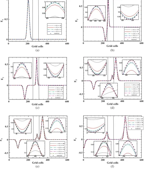
Initially, we consider the case of constant impedance, for which relative permittivity r = 2 and relative permeability μr = 2 are set between cells 250 to 309 (Figure 5). Except this, the medium is considered free space with r = 1 and μr = 1. Computational results are presented after time 0.1251, 0.4378, 0.7505, 1.0632, 1.1258, and 1.5636 ns. Figure 5 shows the electric field propagation. The required number of time steps for varyingν is denoted bynin Figure 5. As shown in Figure 5(b), when the pulse encounters interface 1, it propagates from free space to dielectric medium and is compressed due to change in wave speed. In contrast, when the pulse hits interface 2 (Figure 5(d)), it transits into free space, and the pulse width increases back to the original state (Figure 5(f)). Numerical results are compared with analytical solution for increasing ν 1. The LTS method improves the
(a) (b)
(c) (d)
1
0.5
0
Ey
1
0.5
0
Ey
1
0.5
0
Ey
1
0.5
0
Ey
0 200 400 600
Grid cells
0 200 400 600
Grid cells
0 200 400 600
Grid cells
0 200 400 600
Grid cells v = 0.5, n = 50
v = 2.5, n = 10 v = 6.25, n = 4 v = 12.5, n = 2 Analytical
v = 0.5, n = 175 v = 2.5, n = 35 v = 6.25, n = 14 v = 12.5, n = 7
Analytical v = 43.75, n = 2
v = 0.5, n = 300 v = 2.5, n = 60 v = 6.25, n = 24 v = 12.5, n = 12
Analytical v = 37.5, n = 4
v = 0.5, n = 425 v = 2.5, n = 85 v = 6.25, n = 34 v = 12.5, n = 17
(e) (f) 1
0.5
0
Ey
1
0.5
0
Ey
0 200 400 600
Grid cells
0 200 400 600
Grid cells v = 0.5, n = 450
v = 2.5, n = 95 v = 6.25, n = 36 v = 12.5, n = 18
Analytical v = 37.5, n = 6
v = 112.5, n = 2
v = 0.5, n = 625 v = 2.5, n = 125 v = 6.25, n = 50
v = 12.5, n = 25
Analytical v = 62.5, n = 5 v = 312.5, n = 1
Figure 5. LTS method, Gaussian pulse, Z(x) = Z0. (a) t = 0.1251 ns, (b) t = 0.4378 ns, (c)
t= 0.7505 ns, (d) t= 1.0632 ns, (e) t= 1.1258 ns, (f) t= 1.5636 ns.
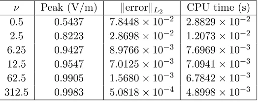
Table 1. Performance of LTS algorithm with varyingν,Z(x) =Z0.
ν Peak (V/m) errorL2 CPU time (s) 0.5 0.5437 7.8448×10⁻² 2.8829×10⁻² 2.5 0.8223 2.8698×10⁻² 1.2073×10⁻² 6.25 0.9427 8.9766×10⁻³ 7.6969×10⁻³ 12.5 0.9547 7.0125×10⁻³ 7.0941×10⁻³ 62.5 0.9905 1.5680×10⁻³ 6.7842×10⁻³ 312.5 0.9983 5.0818×10⁻⁴ 4.8998×10⁻³
resolution and preserves better amplitude of the Gaussian pulse with increasing Courant numberν due to lower discretization errors. The lower discretization errors are a consequence of the fewer explicit time steps required in LTS than that in a standard ν ≤1 propagation. The quantitative performances of LTS method in terms of peak amplitude of transmitted wave and overall errorL2 for varying ν at t= 1.5636 ns are also tabulated in Table 1. The required CPU time (processor IntelRCoreTM i5-2500
CPU @3.30 GHz), measured ins, is reduced with increasing ν as shown in the table. The LTS method requires the change in wave speed because material change is factored in the range of downwind cells to be updated by waves arising out of upwind Riemann problems.
(a) (b)
(c) (d)
(e) (f)
1
0.5
0
Ey
0.5
0
Ey
0.5
0
Ey
0.5
0
Ey
-0.5
0.5
0
Ey
-0.5
0.5
0
Ey
-0.5
0 200 400 600
Grid cells
0 200 400 600
Grid cells
0 200 400 600
Grid cells
0 200 400 600
Grid cells
0 200 400 600
Grid cells
0 200 400 600
Grid cells
v = 0.5, n = 50 v = 2.5, n = 10 v = 6.25, n = 4 v = 12.5, n = 2 Analytical
v = 0.5, n = 175 v = 2.5, n = 35 v = 6.25, n = 14 v = 12.5, n = 7
Analytical v = 43.75, n = 2
v = 0.5, n = 450 v = 2.5, n = 95 v = 6.25, n = 36 v = 12.5, n = 18
Analytical v = 37.5, n = 6
v = 0.5, n = 625 v = 2.5, n = 125 v = 6.25, n = 50 v = 12.5, n = 25
Analytical v = 62.5, n = 5
v = 112.5, n = 2 v = 0.5, n = 300 v = 2.5, n = 60 v = 6.25, n = 24 v = 12.5, n = 12
Analytical v = 37.5, n = 4
v = 0.5, n = 425 v = 2.5, n = 85 v = 6.25, n = 34 v = 12.5, n = 17
Analytical v = 42.5, n = 5
Figure 6. LTS method, Gaussian pulse, Z(x) = Z0. (a) t = 0.1251 ns, (b) t = 0.4378 ns, (c)
Table 2. Performance of LTS algorithm with varyingν,Z(x)=Z0.
ν Et (V/m) Er1 (V/m) Er2 (V/m) errorL2 CPU time (s) 0.5 0.4834 −0.2173 0.1410 7.6155×10⁻² 2.6202×10⁻² 2.5 0.7309 −0.2956 0.2282 2.8872×10⁻² 1.1435×10⁻²
6.25 0.8380 −0.3204 0.2746 1.2244×10⁻² 8.6917×10⁻³ 12.5 0.8486 −0.3245 0.2779 1.1051×10⁻² 7.2581×10⁻³
62.5 0.8804 −0.3313 0.2930 9.1832×10⁻³ 7.1695×10⁻³
Analytical 0.8889 −0.3333 0.2963 -
-preserved for ν 1. Overall CPU time again decreases with increasing ν. In this case, the Courant number ν is limited to 120 based on the self imposed limitation restricting interaction of waves with multiple interfaces to one per time step. The number of time steps decreases with increasing ν again resulting in lower discretization error as ν1 due to LTS.
The previous examples involved unbounded computational domain. In the next example, the
(a) (b)
(c)
50 100 150 200
Grid cells
50 100 150 200
Grid cells
50 100 150 200
Grid cells 0
0.5
0
Ey
0
Ey
-0.5
0.5
0
Ey
-0.5
v = 0.5, n = 170 v = 2.5, n = 34 v = 8.5, n = 10 v = 21.25, n = 4
Analytical v = 42.5, n = 2
v = 0.5, n = 330 v = 2.5, n = 66 v = 16.5, n = 10 v = 27.5, n = 6
Analytical v = 41.25, n = 4 v = 82.5, n = 2
v = 0.5, n = 502 v = 2.51, n = 100 v = 12.55, n = 20 v = 25.1, n = 10
Analytical v = 62.75, n = 4 v = 83.67, n = 3
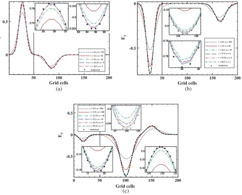
Figure 7. LTS method, Gaussian pulse, Z(x) = Z0, PEC boundaries. (a) t = 0.1418 ns, (b)
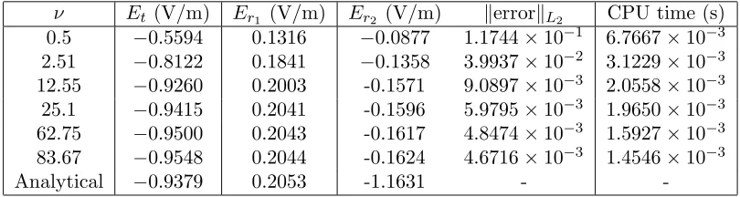
Gaussian pulse propagates in a perfect conducting cavity [14]. The cavity has 200 grid cells with Δx = 0.0005 m, and the first fifty cells have dielectric material with relative permittivity r = 2.3. Other grid cells in the cavity are considered to be free space (r= 1). The Gaussian pulse is initialized at the centre of the domain and is expressed as e−w2t2, wherew = 4.14×10101/s. As time advances the pulse propagates left [14]. The representation of the electric fields after time t = 0.1418,0.2752, and 0.4186 ns are shown in Figure 7. As in the previous case of variable impedance media, when waves originating in a Riemann problem hit a material interface, part of the wave is transmitted, and part reflects back from the interface. These transmitted and reflected waves update appropriate range of downwind and upwind grid cell relative to the interface depending on locally defined wave speed. The computational domain is also bounded with the perfect electric conducting (PEC) boundaries. As shown in Figures 7(b) and 7(c), the outgoing wave from the boundaries completely reflect back into the computational domain so as to haven×E=Ey = 0 at PEC boundaries. This PEC boundary condition implementation was earlier described in detail by the authors in [10] for homogeneous medium. From the results the profile of electric field again agrees very well with the analytical solution forν1. The measured amplitude of transmitted and reflected waves, errorL2, and CPU time for varying ν are again tabulated in Table 3 att= 0.4186 ns. In this tableEtis the amplitude of transmitted wave. The incident pulse initially hits the interface, and the amplitude of reflected wave is Er1 in the table. As shown in Figure 7(b), the left moving transmitted wave after reflection from PEC boundary again hits the dielectric interface. A part of the wave is again reflected from the interface, and amplitude of this reflected wave is represented by Er2 in the table. As in the homogeneous case [10], the discretization error decreases with increase in ν due to decrease in the number of operations with increasing Δt.
Table 3. Performance of LTS algorithm with varyingν,Z(x)=Z0, PEC boundaries.
ν Et (V/m) Er1 (V/m) Er2 (V/m) errorL2 CPU time (s) 0.5 −0.5594 0.1316 −0.0877 1.1744×10⁻¹ 6.7667×10⁻³ 2.51 −0.8122 0.1841 −0.1358 3.9937×10⁻² 3.1229×10⁻³ 12.55 −0.9260 0.2003 -0.1571 9.0897×10⁻³ 2.0558×10⁻³
25.1 −0.9415 0.2041 -0.1596 5.9795×10⁻³ 1.9650×10⁻³ 62.75 −0.9500 0.2043 -0.1617 4.8474×10⁻³ 1.5927×10⁻³ 83.67 −0.9548 0.2044 -0.1624 4.6716×10⁻³ 1.4546×10⁻³
Analytical −0.9379 0.2053 -1.1631 -
-6. CONCLUSIONS
REFERENCES
1. LeVeque, R. J., “Large time step shock-capturing techniques for scalar conservation laws,” SIAM Journal on Numerical Analysis, Vol. 19, No. 6, 1091–1109, 1982, doi: 10.1137/0719080.
2. LeVeque, R. J., “Some preliminary results using a large time step generalization of the Godunov method,” Numerical Methods for the Euler Equations of Fluid Dynamics, edited by F. Angrand et al., 32–47, SIAM, Philadelphia, 1985.
3. LeVeque, R. J., “A large time step generalization of Godunov’s method for system of conservation laws,” SIAM Journal on Numerical Analysis, Vol. 22, No. 6, 1051–1073, 1985, doi: 10.1137/0722063.
4. Qian, Z. and C. Lee, “A class of large time step Godunov schemes for hyperbolic conversation laws and applications,” Journal of Computational Physics, Vol. 230, 7418–7440, 2011, doi: 10.1016/j.jcp.2011.06.008.
5. Guinot, V., “The time-line interpolation method for large-time-step Godunov-type scheme,” Journal Computational Physics, Vol. 177, 394–417, 2002, doi: 10.1006/jcph.2002.7013.
6. Murillo, J., P. Garcia-Navarro, P. Brufau, and J. Burguete, “Extension of an explicit finite volume method tp large time steps (CFL>1): Application to shallow water flows,” Int. J. Numer. Meth. Fluids, Vol. 50, 63–102, 2006, doi: 10.1002/fld.1036.
7. Morales-Hernandez, M., P. Garcia-Navarro, and J. Murillo, “A large time step 1D upwind explicit scheme (CFL >1): Application to shallow water equations,” Journal of Computational Physics, Vol. 231, 6532–6557, 2012, doi: 10.1016/j.jcp.2012.06.017.
8. Morales-Hernandez, M., M. E. Hubbard, and P. Garcia-Navarro, “A 2D extension of a large time step explicit scheme (CFL > 1) for unsteady problems with wet/dry boundaries,” Journal of Computational Physics, Vol. 263, 303–327, 2014, doi: 10.1016/j.jcp.2014.01.019.
9. Xu, R., D. Zhong, B. Wu, X. Fu, and R. Miao, “A large time step Godunov scheme for free-surface shallow water equations,”Chinese Science Bulletin, Vol. 59, 2534–2540, 2014, doi: 10.1007/s11434-014-0374-7.
10. Makwana, N. N. and A. Chatterjee, “Computing with large time steps in time-domain electromagnetics,” Journal of Electromagnetic Waves and Applications, Vol. 37, No. 17, 2182– 2194, 2018, doi: 10.1080/09205071.2018.1500314.
11. LeVeque, R. J.,Finite Volume Methods for Hyperbolic Problems, Cambridge University Press, Cambridge, 2002.
12. LeVeque, R. J., “Convergence of a large time step generalization of Godunov’s method for conservation laws,” Communication on Pure and Applied Mathematics, Vol. 37, 463–477, 1984, doi: 10.1002/cpa.3160370405.
13. Luebbers, R. J., K. S. Kunz, and K. A. Chamberlin, “An interactive demonstration of electromagnetic wave propagation using time domain finite differences,” IEEE Transactions on Education, Vol. 33, No. 1, 66–68, 1990, doi: 10.1109/13.53628.