Solution for Wide Band Scattering Problems by Using the Improved
Ultra-Wide Band Characteristic Basis Function Method
Wen-Yan Nie1 and Zhong-Gen Wang2, *
Abstract—The ultra-wide band characteristic basis function method (UCBFM) is an efficient approach for analyzing wide band scattering problems because ultra-wide characteristic basis functions (UCBFs) can be reused for any frequency sample in the range of interest. However, the errors of the radar cross section calculated by using the UCBFs are usually large at low frequency points. To mitigate this problem, an improved UCBFM is presented. Improved UCBFs (IUCBFs) are derived from primary characteristic basis functions and secondary level characteristic basis functions (SCBFs) by applying a singular value decomposition procedure at the highest frequency point. This method fully considers the mutual coupling effects among sub-blocks to obtain the SCBFs. Therefore, the accuracy is improved at lower frequency points because of the higher quantity of current information contained in the IUCBFs. Numerical results demonstrate that the proposed method is accurate and efficient.
1. INTRODUCTION
Broadband electromagnetic scattering is important in many fields, such as modern radar target recognition, microwave imaging, and microwave remote sensing. One of the most popular methods for calculating the broadband radar cross section (RCS) is the method of moments (MoM) [1]; however, this method is notoriously expensive in terms of computation time and storage requirements when electrically large problems are analyzed. Moreover, it requires the impedance matrix to be generated for each frequency point; hence, if the response over a wide frequency band is of interest, the MoM is computationally intensive. Recently, several techniques have been proposed to alleviate this problem. In [2], the impedance matrix is computed at relatively large frequency intervals and then interpolated to approximate its values. In [3], model-based parameter estimation based on rational function approximation is used to reduce the number of frequency points in which solutions or samples are required in broadband RCS calculation. However, these two techniques must resort to iterative methods, which can cause convergence difficulties when dealing with an ill-conditioned matrix. In [4] and [5], the asymptotic waveform estimation (AWE) technique is proposed to predict the RCS over a band of frequencies. The AWE technique can hardly deal with wide band electromagnetic scattering problems from electrically large objects or multi-objects because it requires MoM matrix inversion at a central frequency. Hence, in [6] and [7], the AWE technique based on the characteristic basis function method (CBFM) [8, 9] is proposed to analyze wide band electromagnetic scattering problems. Although this method avoids solving the MoM matrix using iterative methods, it uses the mutual coupling method to generate characteristic basis functions (CBFs), which is time consuming and memory demanding. In [10], a simple binary search algorithm is described to apply AWE at multiple frequency points to generate an accurate solution over a specified frequency band. The CBFs depend upon the frequency and need to be generated repeatedly for each frequency. Hence, an algorithm called ultra-wide CBFM
Received 8 August 2015, Accepted 29 October 2015, Scheduled 19 December 2015
* Corresponding author: Zhong-Gen Wang ([email protected]).
1 College of Mechanical and Electrical Engineering, Huainan Normal University, Huainan, Anhui 232001, China. 2 College of
(UCBFM) [11, 12] is presented to remove the need to repeatedly generate CBFs for each frequency. The CBFs calculated at the highest frequency after the singular value decomposition (SVD) procedure show electromagnetic behavior at low frequency ranges; these CBFs are called ultra-wide CBFs (UCBFs). Thus, UCBFs can also be employed at lower frequencies without going through the time-consuming step of generating them again. However, the errors of the RCS calculated by using UCBFs are usually large at lower frequency points, its universality is not strong. In [13], improved UCBFs (IUCBFs) are derived from CBFs at the highest frequency point and lowest frequency point. Although accuracy is improved, the amount of calculation increases. In this paper, an improved UCBFM (IUCBFM) is presented. This approach fully considers the mutual effects among sub-blocks and calculates the secondary level CBFs (SCBFs) after the primary CBFs (PCBFs) are obtained. Therefore, IUCBFs contain more current information and have a stronger universality, it could greatly improve the calculation accuracy at lower frequency points.
The remainder of the paper is organized as follows. Section 2 illustrates the UCBFM. Section 3 describes the IUCBFM. Section 4 presents the complexity of the two methods. Section 5 presents the numerical results for four test targets to demonstrate that IUCBFM is accurate and efficient. Section 6 concludes.
2. ULTRA-WIDE CHARACTERISTIC BASIS FUNCTION METHOD
UCBFM [11, 12] begins by modeling the target at the highest frequency point of the desired frequency band and generating the CBFs by using a series of illuminating waves. If we calculate the CBFs at the highest frequency point fh, the geometry of the object is divided into M blocks. These blocks are characterized through a set of CBFs that is constructed by exciting each block with multiple plane waves (PWs). To calculate the CBFs on sub-block i, one must solve the following system:
Zii(fh)JCBF si =VP W si (i= 1,2, . . . , M), (1)
whereZiiis an Nibe×Nibe impedance matrix; VP W si is an Nibe×Npws matrix containing the excitation vector used to illuminate the sub-blocki;Nibe is the number of the RWG basis functions in the extended block i; Npws is the total number of PWs, which is equal to 2NθNφ (including θ- and φ-orthogonal polarizations for each angle). NθandNφdenote the number of different angles in theθandφdirections, respectively. JCBF si is an Nibe ×Npws matrix representing the CBFs. Typically, the number of PWs used to construct the CBFs will exceed the number of degrees of freedom associated with the block. To eliminate the redundant information inJCBF si caused by overestimation, an orthogonalization procedure based on SVD is used to reduce the final number of CBFs. Only CBFs whose relative singular values are above a certain threshold, for example, 1.0E-3, are retained as UCBFs. For simplicity, we assume that all blocks contain the same number ofK UCBFs after SVD, whereK is always smaller thanNpws. The solution to the entire problem is expressed as a linear combination of the M×K UCBFs:
J= M
i=1 K
k=1
αki(fh)JiCBFk, (2)
whereJiCBFk is the kth UCBFs of the blockiand aki the unknown weight coefficients. The solution is obtained at frequencyfh. To obtain theKM unknown expansion coefficients, we substitute Formula (2) into the MoM equationZ•J=V. Thereafter, [JCBFi 1]H, [JCBFi 2]H, . . ., and [JCBFi K]H takes the inner product of both sides of equation Z •J=V, where H stands for conjugated transpose. A reduced matrix can be obtained as follows:
ZR(f)•α(f) =VR(f), (3)
whereZR(f) is the reduced impedance matrix of dimensionKM×KM, each element of which can be expressed as follows:
ZijR(f) =JT •Zij(f)•J i, j < M. (4)
The elements ofVR(f) can be expressed as follows:
VR
Finally, after solving the reduced system in Eq. (3) and substituting the solution back to Eq. (2), one can obtain the solution of the single frequency point. Once generated, these UCBFs, also capture the electromagnetic behavior of lower frequencies and enables one to solve the scattering for any frequency sample in the band without going through the time-consuming process of generating CBFs anew.
3. IMPROVED ULTRA-WIDE CHARACTERISTIC BASIS FUNCTION METHOD
When using the UCBFM, the errors of the RCS calculated by using UCBFs are usually large at low frequency points. To improve the calculation accuracy of UCBFM at lower frequency points, the construction of UCBFs is improved by considering the mutual coupling effects among sub-blocks. A model is established at the highest frequency point fh in the given frequency band, and the number of PWs is reduced. For each plane wave excitation, the SCBFs are calculated after the PCBFs are obtained. The PCBFs of blockican be solved by the following formula.
ZeiiJPi =Vi, (6)
where Vi is the incident field of each block, for i = 1,2, . . . M. Zeii represents the self-impedance of block i, with dimensionality of Ni ×Ni. The PCBFs of block i can be obtained by directly solving Eq. (6). After the PCBFs of each block are solved, according to Foldy-Lax equation theory [14–16], the SCBFs on a block are calculated by replacing the incident field with the scattered fields due to the PCBFs on all blocks except from itself. By solving Eq. (7), we can obtain the first-level SCBFs. Similarly, higher-level SCBFs can be calculated. If the second-level SCBFs is calculated, these SCBFs can be calculated as follows:
ZeiiJSi1 = − M
j=1(j=i)
ZijJPj , (7)
ZeiiJSi2 = − M
j=1(j=i)
ZijJSj1, (8)
We let Nθnew and Nφnew respectively indicate the number of PWs in the θ and φ directions in IUCBFM. 6NθnewNφnew CBFs will exist for each block by considering θ- and φ-polarizations when using IUCBFM (including 2NθnewNφnewJPi , 2NθnewNφnewJSi1 and 2NθnewNφnewJSi2). To reduce the linear dependency among these CBFs, we also need to use an SVD procedure. These three current terms represent different stages in multiple scattering, such that all current solutions JPi , JS1
i , and JSi2 are fed to the SVD procedure separately. To consider the mutual coupling effects among sub-blocks, the IUCBFs contain more current information and the number PWs is reduced.
4. COMPLEXITY ANALYSIS
The computational cost of applying the UCBFM (IUCBFM) involves three parts: firstly is UCBFs construction, then constructing the reduced matrix, and lastly solving the reduced matrix. The most computationally intensive part of the UCBFM is associated with the construction of the UCBFs and the reduced matrix construction procedure.
b. Reduced matrix construction: In UCBFM, the memory requirement and CPU time are with a complexity ofO((KM)2) andO((KM)2N
iNj), respectively. In IUCBFM, the memory requirement and CPU time are with a complexity ofO((KnewM)2) andO((K
newM)2NiNj), respectively. Knew is the number of IUCBFs retained on each block after SVD, whereKnew is always smaller thanK. c. Reduced matrix solution: In UCBFM, the CPU time complexity is O((KM)3). In UCBFM, the
CPU time complexity isO((KnewM)3).
Compared with the UCBFM, the computational complexity of IUCBFM is greatly decreased in UCBFs construction, reduced matrix construction and reduced matrix solution.
5. NUMERICAL RESULTS
To validate the accuracy and efficiency of IUCBFM, three test samples are presented. All simulations are conducted on a personal computer with an Intel(R) Core(TM) i7-3820 CPU with 3.6 GHz (only one core is used) and 32 GB RAM. The second level of the SCBFs is calculated, and the threshold of the SVD is set to 10−3.
First, a PEC cube with a side length of 1 m is considered. We present the result for the problem of scattering over a frequency range from 0.3 GHz to 3 GHz. The geometry is divided into 1110 triangular patches with an average length of λ/10 at 3 GHz, thus resulting in 2786 unknowns. The geometry is sub-divided into 8 blocks, with each block extended by Δ = 0.15λ in all directions. On the basis of Ref. [11], we construct the UCBFs for UCBFM by using a spectrum of PWs incident from 0◦ ≤θ <180◦ and 0◦ ≤φ < 360◦ with Nθ =Nφ = 20. This approach results in 800 CBFs, and 73 UCBFs (average value) are retained on each block after SVD. To prove the high efficiency of the IUCBFs construction, the error convergence curve of UCBFs and IUCBFs with the number of PWs used in the computation is shown in Fig. 1. The relative errorErr is defined as (I−IMOM2/IMOM2)×100%, whereIMOM
is the current coefficient vector computed at 3 GHz by the MoM, andIis the current coefficient vector computed at 3 GHz by the UCBFM or the IUCBFM.•2denotes vector-2 norm. Through a comparison of Err versus the number of PWs given in Fig. 1, we find that the IUCBFM can yield a satisfactory result with a small number of PWs. Compared with the Nθ and Nφ, the Nθnew and Nφnew are reduced to 40%, respectively. In IUCBFM, we illuminate each block with a spectrum of PWs incident from 0◦ ≤ θ < 180◦ and 0◦ ≤ φ < 360◦ with Nθ = Nφ = 8. This approach results in only 384 CBFs for each block, such that the number of CBFs is reduced remarkably. PCBFsJP and SCBFsJS1 and JS2
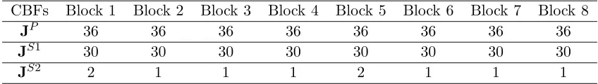
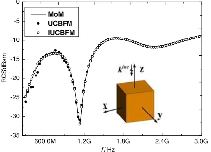
are then fed into the SVD procedure separately. The numbers of JP, JS1, and JS2 retained on each block after SVD are shown in detail in Table 1. A total of 67 IUCBFs (average value) are retained on each block. The bi-static RCSs inθθpolarization calculated by using UCBFM, IUCBFM, and MoM at 600 MHz are shown in Fig. 2. The results calculated by using IUCBFM are more accurate than those calculated by using UCBFM. The broadband RCS (101 frequency sampling points) obtained by using UCBFM and IUCBFM over a frequency range of 0.3 GHz to 3 GHz are shown in Fig. 3. The results at the lower frequency points calculated by using IUCBFM are more accurate than those calculated by using UCBFM.
Table 1. Number of CBFs retained on each block after the SVD of IUCBFM.
CBFs Block 1 Block 2 Block 3 Block 4 Block 5 Block 6 Block 7 Block 8
JP 36 36 36 36 36 36 36 36
JS1 30 30 30 30 30 30 30 30
JS2 2 1 1 1 2 1 1 1
0 100 200 300 400 500 600 700 800 0 100 200 300 400 500 600 700 800 (800, 4.86) Err (%)
Number of the PWs
IUCBFM UCBFM
(384, 4.94)
Figure 1. Error convergence of the current versus the number of PWs.
0 30 60 90 120 150 180
-18 -17 -16 -15 -14 RC S/dBsm θ MoM UCBFM IUCBFM
/( ) ( o φ = 0 )o
Figure 2. Bi-static RCS of the PEC cube at 600 MHz.
600.0M 1.2G 1.8G 2.4G 3.0G
-35 -30 -25 -20 -15 -10 -5 0 RCS /d Bsm
f/ Hz MoM
UCBFM IUCBFM
Figure 3. Broadband RCS of the PEC cube.
600.0M 1.2G 1.8G 2.4G 3.0G
-40 -35 -30 -25 -20 -15 -10 -5 0 5 10 RCS /dBs m
f/ Hz MoM
UCBFM IUCBFM
Figure 4. Broadband RCS of composite PEC conductor.
in all directions and is excited by a spectrum of PWs with Nθ = Nφ = 20 for 800 CBFs. A total of 123 UCBFs are retained on each block after SVD. In IUCBFM, each block is excited by using multiple PWs withNθ=Nφ= 8, and 112 IUCBFs are retained on each block after SVD. The broadband RCS (101 frequency sampling points) obtained by using UCBFM and IUCBFM are shown in Fig. 4. The results at lower frequency points calculated by using IUCBFM are more accurate than those calculated by using UCBFM.
Third, a 252.3744 mm PEC NASA almond with a length of 25 cm over a frequency range of 0.1 GHz to 3 GHz is considered. The geometry is divided into 2684 triangular patches with an average length of
λ/10 at 3 GHz, and this situation leads to 4026 unknowns. The geometry is sub-divided into 4 blocks in the axis x direction. In UCBFM, we construct the UCBFs by using a spectrum of PWs incident from 0◦ ≤θ <180◦ and 0◦≤φ <360◦, withNθ =Nφ= 20. A total of 121 UCBFs (average value) are retained on each block after SVD. In IUCBFM, we construct the IUCBFs at the highest frequency by using a spectrum of PWs incident from 0◦ ≤θ <180◦ and 0◦≤φ <360◦ withNθ=Nφ= 8. A total of 110 IUCBFs (average value) are retained on each block after SVD. The broadband RCS (51 frequency sampling points) calculated by using UCBFM and IUCBFM are shown in Fig. 5. The results at the lower frequency points calculated by using IUCBFM agree more with the MoM than those calculated by using UCBFM.
leading to 15920 unknowns. The structure is divided into 10 blocks; each block is extended by Δ = 0.15λ in all directions. In IUCBFM, each block is excited by using multiple PWs withNθ =Nφ= 8, and 132 IUCBFs are retained on each block after SVD. The broadband RCS (101 frequency sampling points) obtained by using the commercial FEKO and IUCBFM are shown in Fig. 6. It can be seen that the results calculated by IUCBFM agree well with those of FEKO.
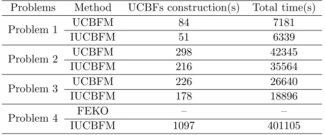
The CPU time of the above four test examples using UCBFM and ICBFM are summarized in Table 2. Compared with the UCBFM, the total time and UCBFs construction time are both reduced when using the IUCBFM. However, we should be noted that when the electrically large problem with more blocks is analyzed, the CPU time will be large. The reason for this is that UCBFM (IUCBFM) needs to reconstruct the reduced matrix at each frequency point. So, it is desirable to use sweep frequency algorithms to further improve the efficiency of UCBFM (IUCBFM).
0.0 500.0M 1.0G 1.5G 2.0G 2.5G 3.0G -60
-45 -30 -15 0
RCS/d
Bsm
f / Hz
MoM UCBFM IUCBFM
Figure 5. Broadband RCS of the NASA PEC almond.
1G 2G 3G 4G 5G 6G
-16 -14 -12 -10 -8
RCS/dBsm
f / Hz
FEKO IUCBFM
Figure 6. Broadband RCS of the PEC cone.
Table 2. CPU time of four problems.
Problems Method UCBFs construction(s) Total time(s)
Problem 1 UCBFM 84 7181
IUCBFM 51 6339
Problem 2 UCBFM 298 42345
IUCBFM 216 35564
Problem 3 UCBFM 226 26640
IUCBFM 178 18896
Problem 4 FEKO – –
IUCBFM 1097 401105
6. CONCLUSION
ACKNOWLEDGMENT
This work was supported by the National Natural Science Foundation of China under Grant No. 61401003, the Specialized Research Fund for the Doctoral Program of Higher Education of China under Grant No. 20123401110006.
REFERENCES
1. Harrington, R. F., Field Computation by Method of Moments, IEEE PRESS, NewYork, 1992. 2. Newman, E. H., “Generation of wide band from the method of moments by interpolating the
impedance matrix,”IEEE Trans. Antennas Propag., Vol. 36, No. 12, 1820–1824, 1988.
3. Burke, G. J., E. K. Miller, S. Chakrabarthi, and K. Demarest, “Using modelbased parameter estimation to increase the efficiency of computing electromagnetic transfer functions”IEEE Trans.
Magn., Vol. 25, No. 4, 2807–2809, 1988.
4. Reddy, C. J., M. D. Deshpande, and C. R. Cockrell, “Fast RCS computation over a frequency band using method of moments in conjunction with asymptotic waveform evaluation technique,” IEEE
Trans. Antennas Propag., Vol. 46, No. 8, 1229–1233, 1998.
5. Zhang, J. P. and J. M. Jin, “Preliminary study of AWE method for FEM analysis of scattering problems,” Microwave Opt. Techno. Lett., Vol. 7, No. 1, 7–12, 1998.
6. Sun, Y. F., Y. Du, and Y. Sao, “Fast computation of wideband RCS using characteristic basis function method and asymptotic waveform evaluation technique”Journal of Electronics (In China), Vol. 27, No. 4, 463–467, 2010.
7. Kucharski, A. A., “Wideband characteristic basis functions in radiation problems,” Radioengineer-ing, Vol. 21, No. 2, 590–596, 2012.
8. Prakash, V. V. S. and R. Mittra, “Characteristic basis function method: A new technique for efficient solution of method of moments matrix equations,” Microw. Opt. Technol. Lett., Vol. 36, No. 2, 95–100, 2003.
9. Degiorgi, M., G. Tiberi, and A. Monorchio, “An SVD-based method for analyzing electromagnetic scattering from plates and faceted bodies using physical optics bases,” IEEE Antennas and
Propagation Society International Symposium, 147–150, Jul. 2005.
10. Zhang, J. P. and J. M. Jin, “Preliminary study of AWE method for FEM analysis of scattering problems,” Microw. Opt. Technol. Lett., Vol. 17, No. 1, 7–12, 1998.
11. Degiorgi, M., G. Tiberi, and A. Monorchio, “Solution of wide band scattering problems using the characteristic basis function method,” IET Microwaves Antennas and Propagation, Vol. 6, No. 1, 60–66, 2012.
12. Degiorgi, M., G. Tiberi, and A. Monorchio, “Wideband scattering through the use of the universal characteristic basis functions(UCBFs),” IEEE Int. Symp. on Antennas and Propagation and
CNCUSNC/URSI Radio Science Meeting, 11–17, Jul. 2010.
13. Zhang, M. Y., Y. F. Sun, and Z. G. Wang, “Solutions of broadband RCS using the characteristic basis function method,” IEEE MTTS International Wireless Symposium, 1–4, Mar. 2015.
14. Tsang, L., C. E. Mandt, and D. H. Ding, “Monte Carlo simulations of the extinction rate of dense media with randomly distributed dielectric spheres based on solution of Maxwell’s equations,”
Optics Letters, Vol. 17, No. 5, 314–316, 1992.
15. Wang, Z. G., Y. F. Sun, and G. H. Wang, “Analysis of electromagnetic scattering from perfect electric conducting targets using improved characteristic basis function method and fast dipole method,”Journal of Electromagnetic Waves and Applications, Vol. 28, No. 7, 893–902, 2014. 16. Sun, Y. F., C. H. Chan, R. Mittra, and L. Tsang, “Characteristic basis function method for solving