Constructing parse forests that include exactly the
n
-best PCFG trees
Pierre Boullier1, Alexis Nasr2and Benoˆıt Sagot1 1. Alpage, INRIA Paris-Rocquencourt & Universit´e Paris 7
Domaine de Voluceau — Rocquencourt, BP 105 — 78153 Le Chesnay Cedex, France {Pierre.Boullier,Benoit.Sagot}@inria.fr
2. LIF, Univ. de la M´editerrann´ee
163, avenue de Luminy - Case 901 — 13288 Marseille Cedex 9, France [email protected]
Abstract
This paper describes and compares two al-gorithms that take as input a shared PCFG parse forest and produce shared forests that contain exactly thenmost likely trees of the initial forest. Such forests are suitable for subsequent processing, such as (some types of) reranking or LFG f-structure computation, that can be per-formed ontop of a shared forest, but that may have a high (e.g., exponential) com-plexity w.r.t. the number of trees contained in the forest. We evaluate the perfor-mances of both algorithms on real-scale NLP forests generated with a PCFG ex-tracted from the Penn Treebank.
1 Introduction
The output of a CFG parser based on dynamic programming, such as an Earley parser (Earley, 1970), is a compact representation of all syntac-tic parses of the parsed sentence, called a shared parse forest (Lang, 1974; Lang, 1994). It can rep-resent an exponential number of parses (with re-spect to the length of the sentence) in a cubic size structure. This forest can be used for further pro-cessing, as reranking (Huang, 2008) or machine translation (Mi et al., 2008).
When a CFG is associated with probabilistic in-formation, as in a Probabilistic CFG (PCFG), it can be interesting to process only thenmost likely trees of the forest. Standard state-of-the-art algo-rithms that extract the n best parses (Huang and Chiang, 2005) produce a collection of trees, los-ing the factorization that has been achieved by the parser, and reproduce some identical sub-trees in several parses.
This situation is not satisfactory since post-parsing processes, such as reranking algorithms or attribute computation, cannot take advantage
of this lost factorization and may reproduce some identical work on common sub-trees, with a com-putational cost that can be exponentally high.
One way to solve the problem is to prune the forest by eliminating sub-forests that do not con-tribute to any of the nmost likely trees. But this over-generates: the pruned forest contains more than the nmost likely trees. This is particularly costly for post-parsing processes that may require in the worst cases an exponential execution time w.r.t. the number of trees in the forest, such as LFG f-structures construction or some advanced reranking techniques. The experiments detailed in the last part of this paper show that the over-generation factor of pruned sub-forest is more or less constant (see 6): after pruning the forest so as to keep the nbest trees, the resulting forest con-tains approximately 103ntrees. At least for some post-parsing processes, this overhead is highly problematic. For example, although LFG parsing can be achieved by computing LFG f-structures on top of a c-structure parse forest with a reason-able efficiency (Boullier and Sagot, 2005), it is clear that a103factor drastically affects the overall speed of the LFG parser.
Therefore, simply pruning the forest is not an adequate solution. However, it will prove useful for comparison purposes.
The new direction that we explore in this pa-per is the production of shared forests that con-tain exactly thenmost likely trees, avoiding both the explicit construction of n different trees and the over-generation of pruning techniques. This can be seen as a transduction which is applied on a forest and produces another forest. The trans-duction applies some local transformations on the structure of the forest, developing some parts of the forest when necessary.
The structure of this paper is the following. Sec-tion 2 defines the basic objects we will be dealing with. Section 3 describes how to prune a shared
forest, and introduces two approaches for build-ing shared forests that contain exactly thenmost likely parses. Section 4 describes experiments that were carried out on the Penn Treebank and sec-tion 5 concludes the paper.
2 Preliminaries
2.1 Instantiated grammars
LetG=hN,T,P, Sibe a context-free grammar (CFG), defined in the usual way (Aho and Ullman, 1972). Throughout this paper, we suppose that we manipulate only non-cyclic CFGs,1 but they may (and usually do) include ε-productions. Given a production p ∈ P, we note lhs(p) its left-hand side, rhs(p)its right-hand side and |p|the length ofrhs(p). Moreover, we noterhsk(p), with1 ≤
k ≤ |p|, the kth symbol of rhs(p). We call
A-production any A-production p ∈ P ofGsuch that
lhs(p) =A.
A complete derivation of a sentence w = t1. . . t|w|(∀i≤ |w|, ti ∈ T) w.r.t.Gis of the form
S ⇒∗
G,w αAβ G,w⇒ αX
1X2. . . Xrβ ⇒∗
G,ww. By
def-inition, A → X1X2. . . Xr is a production of G.
Each of A, X1, X2, . . . , Xr spans a unique oc-currence of a substring ti+1. . . tj ofw, that can
be identified by the corresponding range, noted i..j. A complete derivation represents a parse tree whose yield is w, in which each symbol X of rangei..jroots a subtree whose yield isti+1. . . tj
(i.e., a derivation of the formX ⇒∗
G,wti+1. . . tj).
Let us define thew-instantiation operation (or instantiation). It can be applied to symbols and productions of G, and to G itself, w.r.t. a string w. It corresponds to the well-known intersection of G with the linear automaton that corresponds to the stringw. We shall go into further detail for terminology, notation and illustration purposes.
An instantiated non terminal symbol is a triple notedAi..j whereA ∈ N and0 ≤ i ≤ j ≤ |w|.
Similarly, an instantiated terminal symbol is a triple notedTi..j whereT ∈ T and 0 ≤i ≤j =
i+ 1 ≤ |w|. An instantiated symbol, terminal or non terminal, is noted Xi..j. For any instantiated
symbolXi..j,i(resp. j) is called its lower bound
1
Actually, cyclic CFG can be treated as well, but not cyclic parse forests. Therefore, if using a cyclic CFG which, on a particular sentence, builds a cyclic parse forest, cycles have to be removed before the algorithms descibed in the next sections are applied. This is the case in the SYNTAXsystem (see below).
(resp. upper bound), and can be extracted by the operatorlb()(resp. ub()).
An instantiated production (or instantiated rule) is a context-free production Ai..j →
Xi11..j1Xi22..j2. . . Xirr..jrwhose left-hand side is an instantiated non terminal symbol and whose right-hand side is a (possibly empty) sequence of in-stantiated (terminal or non terminal) symbols, pro-vided the followings conditions hold:
1. the indexes involved are such thati=i1,j=
jr, and∀lsuch that1≤l < r,jl=il+1;
2. the corresponding non-instantiated produc-tion A → X1X2. . . Xr is a production of G.
Iflhs(p) =Ai..j, we setlb(p) =iandub(p) =j.
In a complete derivation S ⇒∗
G,w αAβ G,w⇒
αX1X2. . . Xrβ ⇒∗
G,ww, any symbolXthat spans
the range i..j can be replaced by the instantiated symbols Xi..j. For example, the axiom S can be
replaced by the instantiated axiom S0..|w| in the
head of the derivation. If applied to the whole derivation, this operation creates an instantiated derivation, whose rewriting operations define a particular set of instantiated productions. Given Gandw, the set of all instantiated productions in-volved in at least one complete derivation ofwis unique, and noted Pw. An instantiated derivation
represents an instantiated parse tree, i.e., a parse tree whose node labels are instantiated symbols. In an instantiated parse tree, each node label is unique, and therefore we shall not distinguish be-tween a node in an instantiated parse tree and its label (i.e., an instantiated symbol).
Then, the w-instantiated grammar Gw for G
andwis a CFGhNw,Tw,Pw, S0..|w|isuch that:
1. Pw is defined as explained above;
2. Nw is a set of instantiated non terminal
sym-bols;
3. Twis a set of instantiated terminal symbols.
It follows from the definition ofPwthat
(instan-tiated) symbols of Gw have the following
prop-erties: Ai..j ∈ Nw ⇔ A ⇒∗
G,w ti+1. . . tj, and
Ti..j∈ Tw⇔T =tj.
Thew-instantiated CFGGwrepresents all parse
w.r.t. G.2 In fact, L(G
w) = {w} and the set
of parses of wwith respect to Gw is isomorphic
to the set of parses of w with respect to G, the isomorphism being the w-instantiation operation. The size of a forest is defined as the size of the grammar that represents it, i.e., as the number of symbol occurrences in this grammar, which is de-fined as the number of productions plus the sum of the lengths of all right-hand sides.
Example 1: First running example.
Let us illustrate these definitions by an example. Given the sentencew=the boy saw a man with a telescope and the grammarG(that the reader has in mind), the instantiated productions ofGware:
Det0..1→the0..1 N1..2 →boy1..2
NP0..2 →Det0..1N1..2 V2..3 →saw2..3
Det3..4→a3..4 N4..5 →man4..5
NP3..5 →Det3..4N4..5 Prep5..6 →with5..6
Det6..7→a6..7 N7..8 →telescope7..8
NP6..8 →Det6..7N7..8 PP5..8 →Prep5..6NP6..8
NP3..8 →NP3..5PP5..8 VP2..8 →V2..3NP3..8
VP2..5 →V2..3NP3..5 VP2..8 →VP2..5PP5..8
S0..8 →NP0..2VP2..8
They represent the parse forest ofwaccording to G. This parse forest contains two trees, since there is one ambiguity: VP2..8 can be rewritten in two
different ways.
The instantiated grammar Gw can be
repre-sented as an hypergraph (as in (Klein and Man-ning, 2001) or (Huang and Chiang, 2005)) where the instantiated symbols ofGw correspond to the
vertices of the hypergraph and the instantiated pro-ductions to the hyperarcs.
We define the extension of an instantiated sym-bolXi..j, notedE(Xi..j), as the set of instantiated
parse trees that haveXi..jas a root. The set of all
parse trees ofww.r.t.Gis thereforeE(S0..|w|). In the same way, we define the extension of an in-stantiated production Xi..j → α to be the subset
ofE(Xi..j) that corresponds to derivations of the
formXi..j ⇒
G,wα
∗ ⇒
G,w ti+1. . . tj (i.e., trees rooted
inXi..jand where the daughters of the nodeXi..j
are the symbols ofα).
2.2 Forest traversals
Let us suppose that we deal with non-cyclic forests, i.e., we only consider forests that are
rep-2
In particular, ifGis a binary grammar, itsw-instantation (i.e., the parse forest ofw) has a sizeO(|w|3), whereas it rep-resents a potentially exponential number of parse trees w.r.t |w|since we manipulate only non-cyclic grammars.
resented by a non-recursive instantiated CFG. In this case, we can define two different kinds of for-est traversals.
A bottom-up traversal of a forest is a traversal with the following constraint: anAi..j-production
is visited if and only if all its instantiated right-hand side symbols have already been visited; the instantiated symbol Ai..j is visited once all Ai..j
-productions have been visited. The bottom-up visit starts by visiting all instantiated productions with right-hand sides that are empty or contain only (instantiated) terminal symbols.
A top-down traversal of a forest is a traversal with the following constraint: a nodeAi..j is
vis-ited if and only if all the instantiated productions in which it occurs in right-hand side have already been visited; once an instantiated productionAi..j
has been visited, all itsAi..j-productions are
vis-ited as well. Of course the top-down visit starts by the visit of the axiomS0..|w|.
2.3 Ranked instantiated grammar
When an instantiated grammar Gw = hNw,Tw,Pw, S0..|w|i is built on a PCFG,
ev-ery parse tree in E(S0..|w|) has a probability that is computed in the usual way (Booth, 1969). We might be interested in extracting the kth most
likely tree of the forest represented byGw,3
with-out unfolding the forest, i.e., withwith-out enumerating trees. In order to do so, we need to add some extra structure to the instantiated grammar. The augmented instantiated grammar will be called a ranked instantiated grammar.
This extra structure takes the form ofn-best ta-bles that are associated with each instantiated non terminal symbol (Huang and Chiang, 2005), thus leading to ranked instantiated non terminal sym-bols, or simply instantiated symbols when the con-text is non ambiguous. A ranked instantiated non terminal symbol is writtenhAi..j,T(Ai..j)i, where
T(Ai..j)is then-best table associated with the
in-stantiated symbolAi..j.
T(Ai..j) is a table of at most n entries. The
k-th entry of the table, noted e, describes how to build the k-th most likely tree ofE(Ai..j). This tree will be called thek-th extention ofAi..j, noted Ek(Ai..j). More precisely,eindicates the
instanti-atedAi..j-productionpsuch thatEk(Ai..j)∈ E(p).
It indicates furthermore which trees of the
exten-3In this paper, we shall use thekthmost likely tree and the
sions ofp’s right-hand side symbols must be com-bined together in order to buildEk(Ai..j).
We also define the m, n-extension of Ai..j as
follows: Em,n(Ai..j) =∪m≤k≤nEk(Ai..j).
Example 2: n-best tables for the first running example.
Let us illustrate this idea on our first running ex-ample. Recall that in Example 1, the symbol VP2..8
can be rewritten using the two following produc-tions :
VP2..8 → V2..3 NP3..8
VP2..8 → VP2..5 PP5..8
T(VP2..8)has the following form:
1 P1 VP2..8→V2..3NP3..8 h1,1i 1
2 P2 VP2..8→VP2..5 PP5..8 h1,1i 1
This table indicates that the most likely tree associated with VP2..8 (line one) has probability
P1 and is built using the production VP2..8 →
V2..3 NP3..8 by combining the most likely tree of E(V2..3)(indicated by the first1inh1,1i) with the
most likely tree ofE(NP3..8)(indicated by the
sec-ond 1 in h1,1i). It also indicates that the most likely tree of E(VP2..8) is the most likely tree of E(VP2..8 → V2..3 NP3..8) (indicated by the
pres-ence of 1 in the last column of entry 1) and the second most likely tree of E(VP2..8) is the most
likely tree ofE(VP2..8 → VP2..5 PP5..8). This last
integer is called the local rank of the entry.
More formally, the entryT(Ai..j)[k]is defined
as a 4-tuple hPk, pk, ~vk, lki where k is the rank
of the entry, Pk is the probability of the tree
Ek(Ai..j), pk is the instantiated production such
that Ek(Ai..j) ∈ E(pk), v~k is a tuple of|rhs(pk)|
integers andlkis the local rank.
The tree Ek(Ai..j) is rooted by Ai..j, and its
daughters root N = |rhs(pk)| subtrees that are Ev~k[1](rhs1(pk)), . . . ,Ev~k[N](rhsN(pk)).
Given an instantiated symbol Ai..j and an
in-stantitated production p ∈ P(Ai..j), we define
the n-best table of p to be the table composed of the entrieshPk, pk, ~vk, lkiofT(Ai..j)such that
pk =p.
Example 3: Second running example.
The following is a standard PCFG (probabili-ties are shown next to the corresponding clauses).
S→A B 1
A→A1 0.7 A1→a 1 A→A2 0.3 A2→a 1 B→B1 0.6 B1→b 1 B→B2 0.4 B2→b 1
The instantiation of the underlying (non-probabilistic) CFG grammar by the input text w=a b is the following.
S1..3→A1..2B2..3
A1..2→A11..2 A11..2→a1..2
A1..2→A21..2 A21..2→a1..2
B2..3→B12..3 B12..3→b2..3
B2..3→B22..3 B22..3→b2..3
This grammar represents a parse forest that con-tains four different trees, since on the one hand one can reach (parse) the instantiated terminal symbol a1..2throughA1orA2, and on the other hand one
can reach (parse) the instantiated terminal sym-bolb1..2 throughB1orB2. Therefore, when
dis-cussing this example in the remainder of the paper, each of these four trees will be named accordingly: the tree obtained by reachingathroughAiand b through Bj (i and j are 1 or 2) shall be called Ti,j.
The corresponding n-best tables are trivial (only one line) for all instantiated symbols but A1..2, B2..3 and S1..3. That of A1..2 is the
follow-ing 2-line table.
1 0.7 A→A1 h1i 1 2 0.3 A→A2 h1i 1
The n-best table for B2..3 is similar. The n-best
table for S1..3is:
1 0.42 S1..3 →A1..2B2..3 h1,1i 1
2 0.28 S1..3 →A1..2B2..3 h1,2i 2
3 0.18 S1..3 →A1..2B2..3 h2,1i 3
4 0.12 S1..3 →A1..2B2..3 h2,2i 4
Thanks to the algorithm sketched in section 2.4, these tables allow to compute the following obvi-ous result: the best tree is T1,1, the second-best
tree isT1,2, the third-best tree isT2,1and the worst
tree isT2,2.
Ifn = 3, the pruned forest over-generates: all instantiated productions take part in at least one of the three best trees, and therefore the pruned forest is the full forest itself, which contains four trees.
We shall use this example later on so as to il-lustrate both methods we introduce for building forests that contain exactly thenbest trees, with-out overgenerating.
2.4 Extracting thekth-best tree
is a re-formulation of a procedure originally pro-posed by (Jim´enez and Marzal, 2000). Contrar-ily to (Huang and Chiang, 2005), we shall sketch this algorithm with the terminology introduced above (whereas the authors use the notion of hy-pergraph). The algorithm relies on then-best ta-bles described above: extracting the kth-best tree
consists in extending then-best tables as much as necessary by computing all lines in eachn-best ta-ble up to those that concern thekth-best tree.4
The algorithm can be divided in two sub-algorithms: (1) a bottom-up traversal of the for-est for extracting the bfor-est tree; (2) a top-down traversal for extracting the kth-best tree provided
the(k−1)th
-best has been already extracted. The extraction of the best tree can be seen as a bottom-up traversal that initializes the n-best ta-bles: when visiting a nodeAi..j, the best
probabil-ity of eachAi..j-production is computed by using
the tables associated with each of their right-hand side symbols. The best of these probabilities gives the first line of then-best table forAi..j(the result
for other productions are stored for possible later use). Once the traversal is completed (the instanti-ated axiom has been reached), the best tree can be easily output by following recursively where the first line of the axiom’sn-best table leads to.
Let us now assume we have extracted allk′-best trees, 1 ≤ k′ < k, for a givenk ≤ n. We want to extract thekth-best tree. We achieve this
recur-sively by a top-down traversal of the forest. In or-der to start the construction of thekth-best tree, we
need to know the following:
• which instantiated productionpmust be used for rewriting the instantiated axiom,
• for each ofp’s right-hand side symbolsAi..j,
which subtree rooted in Ai..j must be used;
this subtree is identified by its local rank kAi..j, i.e., the rank of its probability among all subtrees rooted inAi..j.
This information is given by thekthline of the
n-best table associated with the instantiated axiom. If this kth line has not been filled yet, it is
com-puted recursively.5 Once thekth line of then-best
4In the remainder of this paper, we shall use “extracting thekth-best tree” as a shortcut for “extending then-best
ta-bles up to what is necessary to extract thekth-best tree” (i.e., we do not necessarily really build or print thekth-best tree).
5
Because thek−1th-best tree has been computed, thisn -best table is filled exactly up to linek−1. Thekthline is then
table is known, i.e., pand all kAi..j’s are known, the rankkis added top’s so-called rankset, noted ρ(p). Then, the top-down traversal extracts recur-sively for eachAi..jthe appropriate subtree as
de-fined by kAi..j. After having extracted the n-th best tree, we know that a given productionpis in-cluded in thekth-best tree,1≤k≤n, if and only
ifk∈ρ(p).
3 Computing sub-forests that only contain thenbest trees
Given a ranked instantiated grammarGw, we are
interested in building a new instantiated grammar which contains exactly the nmost likely trees of
E(Gw). In this section, we introduce two
algo-rithms that compute such a grammar (or forest). Both methods rely on the construction of new symbols, obtained by decorating instantiated sym-bols ofGw.
An empirical comparison of the two methods is described in section 4. In order to evaluate the size of the new constructed grammars (forests), we consider as a lower bound the so-called pruned forest, which is the smallest sub-grammar of the initial instantiated grammar that includes the n best trees. It is built simply by pruning produc-tions with an empty rankset: no new symbols are created, original instantiated symbols are kept. Therefore, it is a lower bound in terms of size. However, the pruned forest usually overgenerates, as illustrated by Example 3.
3.1 The ranksets method
The algorithm described in this section builds an instantiated grammarGn
w by decorating the
sym-bols of Gw. The new (decorated) symbols have
the form Aρi..j where ρ is a set of integers called a rankset. An integer r is a rank iff we have
1≤r≤n.
The starting point of this algorithm is set of n-best tables, built as explained in section 2.4, with-out explicitely unfolding the forest.
computed as follows: while constructing thek′th-best trees for eachk′between1andk−1, we have identified many pos-sible rewritings of the instantiated axiom, i.e., many (produc-tion, right-hand side local ranks) pairs; we know the proba-bility of all these rewritings, although only some of them con-situte a line of the instantiated axiom’sn-best table; we now identify new rewritings, starting from known rewritings and incrementing only one of their local ranks; we compute (re-cursively) the probability of these newly identified rewritings; the rewriting that has the best probability among all those that are not yet a line of then-best table is then added: it is itskth
A preliminary top-down step uses thesen-best tables for building a parse forest whose non-terminal symbols (apart from the axiom) have the form Aρi..j where ρ is a singleton {r}: the
sub-forest rooted inA{i..jr} contains only one tree, that of local rank r. Only the axiom is not decorated, and remains unique. Terminal symbols are not af-fected either.
At this point, the purpose of the algorithm is to merge productions with identical right-hand sides, whenever possible. This is achieved in a bottom-up fashion as follows. Consider two symbolsAρ1
i..j
and Aρ2
i..j, which differ only by their underlying
ranksets. These symbols correspond to two dif-ferent production sets, namely the set of allAρ1
i..j
-productions (resp. Aρ2
i..j-productions). Each of
these production sets define a set of right-hand sides. If these two right-hand side sets are iden-tical we say thatAρ1
i..jand A
ρ2
i..jare equivalent. In
that case introduce the rankset ρ = ρ1 ∪ρ2 and
create a new non-terminal symbolAρi..j. We now simply replace all occurrences of Aρ1
i..j and A
ρ2
i..j
in left- and right-hand sides by Aρi..j. Of course (newly) identical productions are erased. After such a transformation, the newly created symbol may appear in the right-hand side of productions that now only differ by their left-hand sides; the factorization spreads to this symbol in a bottom-up way. Therefore, we perform this transforma-tion until no new pair of equivalent symbols is found, starting from terminal leaves and percolat-ing bottom-up as far as possible.
Example 4: Applying the ranksets method to the second running example.
Let us come back to the grammar of Example 3, and the same input text w = a b as before. As in Example 3, we consider the case when we are interested in then= 3best trees.
Starting from the instantiated grammar and the n-best tables given in Example 3, the preliminary top-down step builds the following forest (for clar-ity, ranksets have not been shown on symbols that root sub-forests containing only one tree):
S1..3→A{11..}2B{ 1} 2..3
S1..3→A{1}1..2B{2}2..3
S1..3→A{2}1..2B{1}2..3
A{11..}2→A11..2 A11..2→a1..2
A{12..}2→A21..2 A21..2→a1..2
B{21..}3→B12..3 B12..3→b2..3
B{22..}3→B22..3 B22..3→b2..3
In this example, the bottom-up step doesn’t fac-torize out any other symbols, and this is therefore the final output of the ranksets method. It con-tains 2 more productions and 3 more symbols than the pruned forest (which is the same as the origi-nal forest), but it contains exactly the 3 best trees, contrarily to the pruned forest.
3.2 The rectangles method
In this section only, we assume that the grammar Gis binary (and therefore the forest, i.e., the gram-mar Gw, is binary). Standard binarization
algo-rithms can be found in the litterature (Aho and Ull-man, 1972).
The algorithm described in this section per-forms, as the preceding one, a decoration of the symbols of Gw. The new (decorated) symbols
have the form Ax,yi..j, where x and y denote ranks such that 1 ≤ x ≤ y ≤ n. The semantics of the decoration is closely related to the x, y extention ofAi..j, introduced in 2.3:
E(Ax,yi..j) =Ex,y(Ai..j)
It corresponds to ranksets (in the sense of the previous section) that are intervals: Ax,yi..j is
equiv-alent to the previous section’sA{i..jx,x+1,...,y−1,y}. In other words, the sub-forest rooted withAx,yi..j con-tains exactly the trees of the initial forest, rooted withAi..j, which rank range fromxtoy.
The algorithm performs a top-down traversal of the initial instantiated grammarGw. This
traver-sal also takes as input two parametersxand y. It starts with the symbolS0..|w|and parameters1and n. At the end of the traversal, a new decorated for-est is built which contains exactly n most likely the parses. During the traversal, every instantiated symbolAi..j will give birth to decorated
visiting an instantiated symbol or an instantiated production.
3.2.1 Visiting an instantiated symbol
When visiting an instantiated symbol Ai..j with
parameters x and y, a new decorated instan-tiated symbol Ax,yi,j is created and the traver-sal continues on the instantiated productions of P(Ai..j) with parameters that have to be
com-puted. These parameters depend on how the el-ements ofEx,y(Ai..j)are “distributed” among the sets E(p)with p ∈ P(Ai..j). In other words, we
The idea can be easily illustrated on an exam-ple. Suppose we are visiting the instantiated sym-bolAi..j with parameters 5and10. Suppose also
that Ai..j can be rewritten using the two
instanti-ated productions p1 and p2. Suppose finally that
the5to10entries ofT(Ai..j)are as follows6: 5th most likely analysis of
E(Ai..j)is the4th most
likely analysis of E(p1) and E6(Ai..j) = E2(p2)
and so on. From this table we can deduce that:
E5,10(Ai..j) =E4,6(p1)∪ E2,4(p2)
The traversal therefore continues onp1 and p2
with parameters4,6and2,4.
3.2.2 Visiting an instantiated production When visiting an instantiated production pof the formAi..j → Bi..l Cl..j with parametersx andy,
a collection ofqinstantiated productionsprof the
form Ax,yi..j → Bx1r,x2r
i..l C
y1
r,y2r
l..j , with 1 ≤ r ≤ q,
are built, where the parameters x1
r, x2r, yr1, y2r and
qhave to be computed.
Once the parameters q and x1r, x2r, y1r, yr2 with
1 ≤ r ≤ q, have been computed, the traversal continues independently on Bi..l with parameters
x1randx2rand onCl..j with parametersy1randyr2.
6Only the relevant part of the table have been kept in the figure.
The computation of the parameters x1r, x2r, y1r andyr2for1≤r≤q, is the most complex part of the algorithm, it relies on the three notions of rect-angles, q-partitions and n-best matrices, which are defined below.
Given a 4-tuple of parameters x1r, x2r, y1r, y2r, a rectangle is simply a pairing of the form
hhx1r, x2ri,hyr1, yr2ii. A rectangle can be interpreted as a couple of rank ranges : hx1
r, y1riandhx2r, yr2i.
It denotes the cartesian productx1
r, x2r
be a collection ofq rectangles. It will be called a q-partition of the instantiated production piff the following is true:
To put it differently, this definition means that
hhx11, x21i,hy11, y12ii, . . . ,hhx1q, x2qi,hy1q, y2qii is aq partition of p if any tree of E(Bx1r,x2r
i..l ) combined
with any tree ofE(Cy1r,y2r
l..j )is a tree ofEx,y(p)and,
conversely, any tree ofEx,y(p)is the combination
of a tree ofE(Bx1r,x2r
i..l )and a tree ofE(C
y1
r,yr2
l..j ).
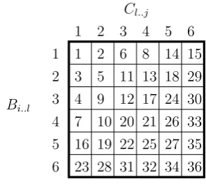
The n-best matrix associated with an instanti-ated productionp, introduced in (Huang and Chi-ang, 2005), is merely a two dimensional represen-tation of then-best table ofp. Such a matrix, rep-resents how the n most likely trees of E(p) are built. An example of an n-best matrix is repre-sented in figure 1. This matrix says that the first most likely tree of p is built by combining the tree E1(Bi..l) with the treeE1(Cl..j) (there is a1
in the cell of coordinate h1,1i). The second most likely tree is built by combining the treeE1(Bi..l)
andE2(Cl..j)(there is a2in the cell of coordinate
M(i, y)< M(x, y)∀i1≤i < x M(x, j) < M(x, y)∀j1≤j < y
Given ann-best matrixM of dimensions d = X·Y and two integersxandysuch that1≤x < y≤d,M can be decomposed into three regions:
• the lower region, composed of the cells which contain ranksiwith1≤i < x
• the intermediate region, composed of the cells which contain ranksiwithx≤i≤y
• the upper region, composed of the cells which contain ranksisuch thaty < i≤d.
The three regions of the matrix of figure 1, for x = 4andy = 27have been delimited with bold
Figure 2: Decomposition of ann-best matrix into a lower, an intermediate and an upper region with parameters4and27.
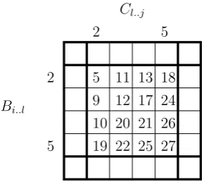
It can be seen that a rectangle, as introduced earlier, defines a sub-matrix of then-best matrix. For example the rectangle hh2,5i,h2,5ii defines the sub-matrix which north west corner isM(2,2) and south east corner isM(5,5), as represented in figure 3.
When visiting an instantiated productionp, hav-ingM as ann-best matrix, with the two parame-ters x and y, the intermediate region of M, with respect toxand y, contains, by definition, all the ranks that we are interested in (the ranks rang-ing from x to y). This region can be partitioned into a collection of disjoint rectangular regions. Each such partition therefore defines a collection of rectangles or aq-partition.
The computation of the parameters x1
r, yr1, x2r
and y2r for an instantiated production p therefore boils down to the computation of a partition of the intermediate region of then-best matrix ofp.
9
Figure 3: The sub-matrix corresponding to the rectanglehh2,5i,h2,5ii
We have represented schematically, in figure 4, two 4-partitions and a 3-partition of the interme-diate region of the matrix of figure 2. The left-most (resp. rightleft-most) partition will be called the vertical (resp. horizontal) partition. The middle partition will be called an optimal partition, it de-composes the intermediate region into a minimal number of sub-matrices.
Figure 4: Three partitions of ann-best matrix
The three partitions of figure 4 will give birth to the following instantiated productions:
a simple heuristic has been used which computes horizontal and vertical partitions and keeps the partition with the lower number of parts.
The size of the new forest is clearly linked to the partitions that are computed: a partition with a lower number of parts will give birth to a lower number of decorated instantiated productions and therefore a smaller forest. But this optimization is local, it does not take into account the fact that an instantiated symbol may be shared in the initial forest. During the computation of the new forest, an instantiated production p can therefore be vis-ited several times, with different parameters. Sev-eral partitions ofpwill therefore be computed. If a rectangle is shared by several partitions, this will tend to decrease the size of the new forest. The global optimal must therefore take into account all the partitions of an instantiated production that are computed during the construction of the new for-est.
Example 5: Applying the rectangles method to the second running example.
We now illustrate more concretely the rectan-gles method on our second running example intro-duced in Example 3. Let us recall that we are in-terested in then= 3best trees, the original forest containing 4 trees.
As said above, this method starts on the instan-tiated axiom S1..3. Since it is the left-hand side
of only one production, this production is visited with parameters1,3. Moreover, itsn-best table is the same as that of S1..3, given in Example 3. We
show here the corresponding n-best matrix, with the empty lower region, the intermediate region (cells corresponding to ranks 1 to 3) and the upper region:
As can be seen on that matrix, there are two op-timal 2-partitions, namely the horizontal and the vertical partitions, illustrated as follows:
II I II I
Let us arbitrarily chose the vertical partition. It gives birth to twoS1..3-productions, namely:
S1,3
Since this is the only non-trivial step while apply-ing the rectangles algorithm to this example, we can now give its final result, in which the axiom’s (unnecessary) decorations have been removed:
S1..3→A11,..22B{
Compared to the forest built by the ranksets algo-rithm, this forest has one less production and one less non-terminal symbol. It has only one more production than the over-generating pruned for-est.
4 Experiments on the Penn Treebank
The methods described in section 3 have been tested on a PCFGGextracted from the Penn Tree-bank (Marcus et al., 1993). Ghas been extracted naively: the trees have been decomposed into bi-nary context free rules, and the probability of ev-ery rule has been estimated by its relative fre-quency (number of occurrences of the rule divided by the number of occurrences of its left hand side). Rules occurring less than 3 times and rules with probabilities lower than3×10−4have been
elim-inated. The grammar produced contains 932 non terminals and3,439rules.7
The parsing has been realized using the SYN
-TAXsystem which implements, and optimizes, the Earley algorithm (Boullier, 2003).
The evaluation has been conducted on the1,845 sentences of section 1, which constitute our test set. For every sentence and for increasing values ofn, ann-best sub-forest has been built using the rankset and the rectangles method.
The performances of the algorithms have been measured by the average compression rate they
7
0e+00 1e+05 2e+05 3e+05 4e+05 5e+05 6e+05 7e+05 8e+05 9e+05
0 100 200 300 400 500 600 700 800 900 1000
avg. nb of trees in the pruned forest
n
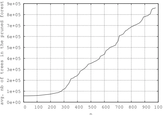
Figure 5: Overgeneration of the prunedn-best forest
1 10 100 1000
1 10 100 1000
compression rate
n pruned forest
rectangles ranksets
Figure 6: Average compression rates
achieve for different values of n. The compres-sion rate is obtained by dividing the size of the n-best sub-forest of a sentence, as defined in sec-tion 2, by the size of the (unfolded) n-best forest. The latter is the sum of the sizes of all trees in the forest, where every tree is seen as an instantiated grammar, its size is therefore the size of the corre-sponding instantiated grammar.
The size of then-best forest constitutes a natu-ral upper bound for the representation of then-best trees. Unfortunately, we have no natural lower bound for the size of such an object. Neverthe-less, we have computed the compression rates of the prunedn-best forest and used it as an imperfect lower bound. As already mentioned, its imper-fection comes from the fact that a pruned n-best
forest contains more trees than the n best ones. This overgeneration appears clearly in Figure 5 which shows, for increasing values of n, the av-erage number of trees in then-best pruned forest for all sentences in our test set.
Figure 6 shows the average compression rates achieved by the three methods (forest pruning, rectangles and ranksets) on the test set for increas-ing values ofn. As predicted, the performances lie between1(no compression) and the compression of then-best pruned forest. The rectangle method outperforms the ranksets algorithm for every value ofn.
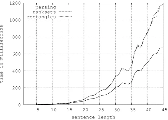
0 200 400 600 800 1000 1200
5 10 15 20 25 30 35 40 45
time in milliseconds
sentence length parsing
ranksets rectangles
Figure 7: Processing time
time for sentences of a given length, as well as the average time necessary for building the 100-best forest using the two aforementioned algorithms. This time includes the parsing time i.e. it is the time necessary for parsing a sentence and build-ing the100-best forest. As shown by the figure, the time complexities of the two methods are very close.
5 Conclusion and perspectives
This work presented two methods to build n-best sub-forests. The so called rectangle meth-ods showed to be the most promising, for it al-lows to build efficient sub-forests with little time overhead. Future work will focus on computing optimized partitions of then-best matrices, a cru-cial part of the rectangle method, and adapting the method to arbitrary (non binary) CFG. Another line of research will concentrate on performing re-ranking of then-best trees directly on the sub-forest.
Acknowledgments
This research is supported by the French National Research Agency (ANR) in the context of the SEQUOIA project (ANR-08-EMER-013).
References
Alfred V. Aho and Jeffrey D. Ullman. 1972. The Theory of Parsing, Translation, and Compiling,
vol-ume 1. Prentice-Hall, Englewood Cliffs, NJ.
Taylor L. Booth. 1969. Probabilistic representation of formal languages. In Tenth Annual Symposium on
Switching and Automata Theory, pages 74–81.
Pierre Boullier and Philippe Deschamp. 1988. Le syst`eme SYNTAXTM - manuel d’utilisation. http://syntax.gforge.inria.fr/syntax3.8-manual.pdf.
Pierre Boullier and Benot Sagot. 2005. Efficient and robust LFG parsing: SXLFG. In Proceedings of IWPT’05, Vancouver, Canada.
Pierre Boullier. 2003. Guided Earley parsing. In
Pro-ceedings of IWPT’03, pages 43–54.
Jay Earley. 1970. An efficient context-free parsing algorithm. Communication of the ACM, 13(2):94– 102.
Liang Huang and David Chiang. 2005. Better k-best parsing. In Proceedings of IWPT’05, pages 53–64.
Liang Huang. 2008. Forest reranking: Discriminative parsing with non-local features. In Proceedings of
ACL’08, pages 586–594.
V´ıctor M. Jim´enez and Andr´es Marzal. 2000. Com-putation of the n best parse trees for weighted and stochastic context-free grammars. In Proceedings
of the Joint IAPR International Workshops on Ad-vances in Pattern Recognition, pages 183–192,
Lon-don, United Kingdom. Springer-Verlag.
Dan Klein and Christopher D. Manning. 2001. Parsing and hypergraphs. In Proceedings of IWPT’01.
Bernard Lang. 1974. Deterministic techniques for ef-ficient non-deterministic parsers. In J. Loeckx, ed-itor, Proceedings of the Second Colloquium on
Au-tomata, Languages and Programming, volume 14 of Lecture Notes in Computer Science, pages 255–269.
Bernard Lang. 1994. Recognition can be harder then parsing. Computational Intelligence, 10:486–494.
Mitchell P. Marcus, Beatrice Santorini, and Mary Ann Marcinkiewicz. 1993. Building a large annotated corpus of English: The Penn treebank.
Computa-tional Linguistics, 19(2):313–330, June.