A Thesis Submitted for the Degree of PhD at the University of Warwick
http://go.warwick.ac.uk/wrap/49186
This thesis is made available online and is protected by original copyright. Please scroll down to view the document itself.
by
Shavak Sinanan
Thesis
Submitted to The University of Warwick
for the degree of
Doctor of Philosophy
Mathematics Institute
List of Tables vii
List of Algorithms viii
Listings ix
Acknowledgements x
Declaration xiii
Abstract xiv
Notation xv
1 Introduction 1
1.1 The Class of Polycyclic-by-Finite Groups . . . 1
1.2 Overview of Project . . . 2
1.2.1 Objectives . . . 2
1.2.2 Results . . . 3
1.2.3 Notes and Assumptions . . . 5
2 Background Material 6 2.1 Permutation Groups . . . 6
2.1.1 Definitions and Notation . . . 7
2.1.2 Computation of Orbits and Stabilisers . . . 8
2.1.3 Bases and Strong Generating Sets . . . 11
2.2 Polycyclic Groups . . . 17
2.2.1 Finite Soluble Groups . . . 19
2.2.2 Infinite Polycyclic Groups . . . 21
2.3 Representation Theory and Extensions . . . 22
2.3.1 The Terminology of Representation Theory . . . 23
2.3.2 Semidirect Products, Complements, Derivations and First Co-homology Groups . . . 24
2.3.3 Extensions of Modules and The Second Cohomology Group . 26 3 Multiplication 29 3.1 Representation of Elements . . . 30
3.1.1 The Normal Form . . . 30
3.1.2 The Multiplication Problem . . . 31
3.2 The Multiplication Algorithm . . . 32
3.2.1 Strategy . . . 32
3.2.2 Data . . . 33
3.2.3 The Algorithm . . . 37
3.3 Applications . . . 44
3.3.1 Transversal Images . . . 45
3.3.2 Element Inversion . . . 45
3.3.3 Orders of Elements . . . 46
3.3.4 Transfer to the Category of Polycyclic Groups . . . 46
4 Subgroups 50 4.1 The Subgroup Generation Problem . . . 51
4.2 Construction . . . 52
4.2.2 Data . . . 64
4.2.3 Membership Testing . . . 66
4.3 Applications . . . 67
4.3.1 The Soluble Radical . . . 67
4.3.2 Sylow Subgroups . . . 68
5 Conjugacy 70 5.1 The Centre . . . 71
5.2 The Conjugacy Problem . . . 75
5.2.1 Centralisers . . . 75
5.2.2 Conjugacy Testing . . . 80
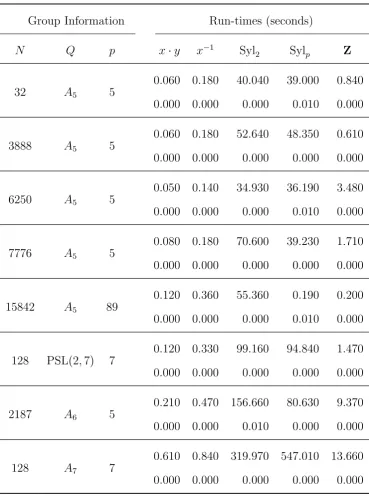
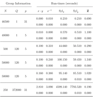
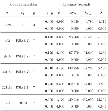
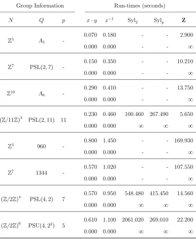
6 Conclusion 83 6.1 Examples and Run-times . . . 83
6.2 Implementation . . . 101
6.2.1 List of Functions . . . 101
6.2.2 Technical Considerations . . . 102
6.2.3 Native Support . . . 103
6.3 Future Work . . . 104
A Package Documentation 106 A.1 Introduction . . . 106
A.2 Getting Started . . . 106
A.3 Creation of a Group . . . 107
A.3.1 Construction Functions . . . 107
A.4 Basic Group Properties . . . 107
A.4.1 Infrastructure . . . 107
A.4.2 Numerical Invariants . . . 108
A.5 Elements . . . 108
A.5.1 Definition of Elements . . . 109
A.5.2 Arithmetic Operations on Elements . . . 109
A.5.3 Properties of Elements . . . 110
A.5.4 Predicates for Elements . . . 110
A.5.5 Set Operations . . . 111
A.6 Subgroups . . . 111
A.6.1 Definition of Subgroups by Generators . . . 112
A.6.2 Membership and Coercion . . . 112
A.6.3 Standard Subgroup Constructions . . . 112
A.6.4 Sylow Subgroups . . . 113
A.6.5 Centralisers . . . 113
A.7 Normal Subgroups and Subgroup Series . . . 113
A.7.1 Normal Structure . . . 113
A.7.2 Characteristic Subgroups . . . 113
A.7.3 Subgroup Series . . . 114
A.8 Conjugacy . . . 114
A.9 Transfer Between Group Categories . . . 114
A.9.1 Transfer to GrpPC or GrpGPC . . . 114
B Program Listing 116
6.1 Run-times for perfect groups . . . 95
6.2 Run-times for subgroups of AGLp3,5q. . . 96
6.3 Run-times for subgroups of AGLp4,3q. . . 97
6.4 Run-times for reducible matrix groups . . . 98
6.5 Run-times for module extensions . . . 99
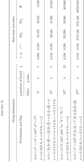
6.6 Run-times for finitely presented groups that map onto A5 . . . 100
3.1 Element Multiplication . . . 42 4.1 Sifting . . . 55 4.2 Standard version of the extended Schreier–Sims algorithm . . . 59 4.3 Normal closure version of the extended Schreier–Sims algorithm . . . 63 4.4 Base-preserving version of the extended Schreier–Sims algorithm . . . 65 5.1 Finding the centre . . . 74 5.2 Finding centralisers . . . 79 5.3 Testing Element Conjugacy . . . 82
B.1 grputils.m . . . 116
B.2 permsv.m . . . 117
B.3 recfrmtdef.m . . . 122
B.4 permdata.m . . . 124
B.5 pcbfconstruct.m . . . 130
B.6 pcbfarithmetic.m . . . 159
B.7 pcbfcattrans.m . . . 173
B.8 pcbfschreiersims.m . . . 180
B.9 pcbfsubgroup.m . . . 197
B.10 pcbfderived.m . . . 213
B.11 pcbfsylow.m . . . 218
B.12 pcbfcentre.m . . . 221
B.13 pcbfcentraliser.m . . . 225
B.14 pcbfconjugacy.m . . . 229
B.15 pcbfmain.m . . . 233
First and foremost I would like to express my deepest gratitude to my supervisor, Prof. Derek Holt, who has, at all times, been a source of inspiration and encourage-ment. Derek has been an excellent supervisor, and is an outstanding mathematician. His keen insights and sharp observations have always kept me interested and mo-tivated, and I owe every ounce of mathematical knowledge and skill that I have acquired over the last four years to him.
A key ingredient to success is a productive, challenging yet comfortable environ-ment, and I am fortunate to have found that and so much more in, where I now call my mathematical home, the Warwick Mathematics Institute. The support provided by the Institute is all that one could hope for as a graduate student, and I wish to sincerely thank the staff for the magnificent job that they have done, and continue to do, in managing us mathematicians. Special mention must be made of the cur-rent and former Postgraduate Coordinators, Carole Fisher and Carol Wright, for whose patience and understanding over the last four years I am eternally grateful. I would also like to acknowledge the University of Warwick for the financial support that I have received via the Warwick Postgraduate Scholarship and the Chancellor’s International Scholarship during my time as a doctoral candidate.
I must also express my gratitude to Prof. John Cannon of the Computational Algebra Group at the University of Sydney, for providing me with the opportunity to visit Sydney to collaborate directly with the Magma developers, and for his keen interest in my work.
earlier academic development, in particular I would like to mention Prof. Michael Vaughan-Lee of Christ Church College, Oxford, and Prof. E. J. Farrell of the Uni-versity of the West Indies, St. Augustine.
As I near the end of my time at Warwick, I think about the reasons why I am where I am now, and there are just two: Avory and Ousha. To my parents: your unwavering support at all stages of my life means more to me than you shall ever know, and you will always be the reason why I am where I am.
A famous quote of William Butler Yeats goes: “Think where man’s glory most begins and ends, and say my glory was I had such friends.” To those most important to me:
Rajiv ‘Fliz’ Sinanan — “You’re the best man I know.” Rishi ‘Ding’ Ramsumair — C c a l 3. SBW. Blauuw.
Travers ‘JT’ Sinanan — “Be resourceful man. Bring me some champagne and oysters.”
Kerwin ‘The Prophet’ Cumberbatch — Salaam brother Numsi. Avinash ‘T.C.’ Ramdass — The real man in short pants. Shivana ‘Tea Poog’ Maharaj — For F.R.I.E.N.D.S and crˆepes. Mandana ‘Mana Joon’ Namdar — For halloumi cheese distractions! Tasneem ‘Joggers’ Sharafally — Gorillas, Shirts and Permitted. Andrew ‘Koopa Troopa’ Ferguson — Red shell first, cigar later. Shivani ‘Nanny Goat’ Jacelon — You’re ugly.
Sasha ‘The Popo’ Nath — For Jay Sean and Apple Sourz bonding. Machel Pantin — B +O + B + Any punch button.
Anja Dass — Wha’s the scene horse?
Megan ‘Chinchilla’ Lee Yuen — For Chinese delights. Clint ‘Tuffzool’ Sieunarine — My brother of the sword. Michael Dor´e — Time for an I.M.O. Q6?
one has ever deserved.
The author declares that the material contained in this thesis is entirely his own work. As is standard practice, the subject matter developed builds on existing theory, and clear citations and references are provided where necessary.
Although material contained herein may be submitted for publication at a later date, the author has not published any work which forms part of this thesis.
No part of this thesis has been submitted, for the purposes of a degree or other-wise, to any other university or educational institution.
A set of fundamental algorithms for computing with polycyclic-by-finite groups is presented here. Polycyclic-by-finite groups arise naturally in a number of contexts; for example, as automorphism groups of large finite soluble groups, as quotients of finitely presented groups, and as extensions of modules by groups.
No existing mode of representation is suitable for these groups, since they will typically not have a convenient faithful permutation representation.
A mixed mode is used to represent elements of such a group; utilising a polycyclic presentation or a power-conjugate presentation for the elements of the normal subgroup, and a permutation representation for the elements of the quotient.
Z the set of integers, t. . . ,1,0,1, . . .u Z the set of positive integers, t1,2, . . .u Z the set of negative integers, t. . . ,2,1u Zn, Z{nZ the set of integers modulo n
N the set of natural numbers, t0,1, . . .u
Fpn the finite field of order pn where p is prime andn PZ GLpd, Rq the group of invertible dd matrices over a ring,R
SLpd, Rq the group of dd matrices with determinant 1 over a ring, R
PGLpd, qq the projective general linear group of degreed over the field, Fq, q a prime power
PSLpd, qq the projective special linear group of degreed over the field, Fq, q a prime power
GUpd, q2q the general unitary group of degree d over the field,
Fq2, q a
prime power
SUpd, q2q the special unitary group of degree d over the field,
Fq2, q a
prime power
PGUpd, q2q the projective general unitary group of degree d over the
field, Fq2, q a prime power
PSUpd, q2q the projective special unitary group of degreedover the field, Fq2, q a prime power
AGLpd, qq the group corresponding to the action of GLpd,Fqq on the affine points of thed-dimensional vector space over the field, Fq, q a prime power
[3. . .8] the array, [3, 4, 5, 6, 7, 8] [11. . .1 by 3] the array, [11, 8, 5, 2, 1]
Introduction
This chapter aims to acquaint the reader with the topic and scope of the research undertaken towards the completion of this thesis. Firstly, the class of polycyclic-by-finite groups is discussed briefly, after which the objectives and results of the project are outlined.
1.1
The Class of Polycyclic-by-Finite Groups
Let P and Q be properties of groups. A group is said to be poly-P if it admits a finite subnormal series such that every factor group has property P. A group, G, is a P-by-Q group if it has a normal subgroup, N, such that N has property P, and G{N has property, Q.
Thus, a group ispolycyclic-by-finiteif it has a normal polycyclic subgroup of finite index. That is, if it has normal subgroup of finite index that admits a subnormal series with cyclic factors.
Segal (1983) proves that the property “polycyclic-by-finite” is equivalent to the properties:
(i) poly-(cyclic or finite),
(ii) (poly-C8)-by-finite,
where C8 is the property of being infinite cyclic.
By a well-known theorem of P. Hall, every polycyclic-by-finite group is finitely presented — and in fact, polycyclic-by-finite groups form the largest known section-closed class of finitely presented groups. It is this fact that makes polycyclic-by-finite groups natural objects of study from the algorithmic standpoint. For an excellent theoretical account of the algorithmic decision theory of polycyclic-by-finite groups, the reader is referred to (Baumslag et al., 1991).
In contrast to the paper of Baumslag et al. (1991), this thesis explores the com-putational properties of polycyclic-by-finite groups from a practical perspective, at-tempting to produce algorithms which are conducive to computer implementation.
In this context, the algorithms developed are targeted not only at infinite polycyclic-by-finite groups, but, in fact, primarily at finite insoluble groups with a large soluble normal subgroup, as such groups do not often have a convenient permutation rep-resentation. These groups, although trivially polycyclic-by-finite, may be viewed as polycyclic-by-finite with non-trivial polycyclic normal subgroup, leading to a com-putationally effective representation. Groups of this type arise naturally in many applications such as automorphism groups of large finite soluble groups, as quotients of finitely presented groups, and as extensions of modules by groups.
1.2
Overview of Project
The objectives and outcome of the research governing this thesis are outlined in this section.
1.2.1
Objectives
the computer. Fundamental algorithms for a class of groups include algorithms to perform the tasks of multiplication, element inversion and subgroup generation.
The material developed also aims to use the fundamental algorithms developed to perform more advanced structural computations in polycyclic-by-finite groups such as finding Sylow subgroups (in the finite case), computing centralisers and testing element conjugacy.
Focus was initially restricted to finite insoluble groups, as many of the interesting examples of polycyclic-by-finite groups that arise in practice are in fact finite (see Section 1.1). However, taking into account the recent developments and ongoing research in the area of computing with infinite polycyclic groups (see Eick, 2001), it was deemed prudent to allow for the possibility of infinite groups, and the parameters of the problem were broadened accordingly.
1.2.2
Results
This subsection contains a synopsis of the results emerging from this thesis.
Theoretical
The main body of the thesis begins by defining a normal form for the elements of a polycyclic-by-finite group, after which, a data structure which facilitates multiplica-tion of elements is introduced. This material forms the content of Chapter 3, which culminates with a detailed description of the multiplication algorithm.
A selection of advanced structural computations in polycyclic-by-finite groups is discussed in Chapter 5. Specifically, algorithms to compute the centre of the group and the centraliser of an element are presented, along with a constructive method to test element conjugacy. Substantial use of linear algebra and representation theory is made here.
Practical
In keeping with the “machine implementable” ethos of this course of research, every function described in thesis has been fully implemented using the Magma Computa-tional Algebra System1. This suite of functions forms a major portion of a complete
package for computing with polycyclic-by-finite groups in Magma. The implemen-tation was done in parallel with the development of the algorithms, and forms a significant part of the project.
An up-to-date version of the source code (written in the Magma language) fulfill-ing the implementation may be found on the compact disc accompanyfulfill-ing this thesis. The reader should consult the documentation provided Appendix A for directions on how to load and use the package. Some example computations are given in Sec-tion 6.1 of Chapter 6. Although extensive testing has been done, the implementaSec-tion is still in developmental stage and, in rare circumstances, bugs may arise, especially when attempting to compute with infinite polycyclic-by-finite groups. Source code listings are given in Appendix B.
1Magma is a large, well-supported software package designed for computations in algebra, number theory, algebraic geometry and algebraic combinatorics. See
1.2.3
Notes and Assumptions
Existing Computational Representations
At points in the thesis, the reader may encounter the phrase “without performing any element arithmetic in E”, where E is a polycyclic-by-finite group. This simply means that, while there exists some (possibly inefficient) representation forE on the computer, this representation is not used to perform element arithmetic. Indeed, the first and most important goal of the theory is to set up machinery so that elements of E can be manipulated by performing operations only within the normal polycyclic subgroup and the associated finite quotient, without appealing to any existing representation of E.
On a related point, while, for a given polycyclic-by-finite group, E, there may be many different decompositions ofE as an extension of a polycyclic group by a finite group, the algorithms presented in this thesis are targeted at those decompositions in which the finite quotient is relatively small and therefore admits a permutation representation of manageable degree. Thus, it shall hereinafter be assumed that the polycyclic-by-finite groups in this thesis can be so decomposed.
Complexity
Background Material
This chapter contains a summary of the required background material, and intro-duces notation that is used throughout the rest of the thesis.
2.1
Permutation Groups
Permutation group algorithms are among the best developed parts of computational group theory. The base and strong generating set data structure and the Schreier– Sims algorithm introduced by Sims (1970, 1971) form the backbone of this area, and the resulting methods enable detailed structural computations to be carried out routinely in permutation groups of degree up to about 107.
As discussed in Chapter 1, the chosen representation for polycyclic-by-finite groups involves viewing the finite quotients primarily as permutation groups. Thus, the algorithms developed here for polycyclic-by-finite groups rely on the existing and well established methods for manipulating finite groups of permutations; the fundamental concepts of which are presented in this section. For a detailed account of the material discussed here, the reader is referred to (Holt et al., 2005, Chap. 4) and (Seress, 2003).
2.1.1
Definitions and Notation
In the context of permutation groups, the notation used is similar to that of Seress (2003) and Holt et al. (2005). The required definitions are reproduced concisely here.
The cycle notation shall be used for permutations, with the identity permutation denoted by pq. The group of all permutations of an n-element set, Ω, is denoted by SympΩq, or Sn if only the size of Ω is relevant. The image of α P Ω under the permutation g P SympΩq is written as αg. The alternating group on Ω is denoted by AltpΩq (or An in the case of a generic n-element set). The support of g P SympΩq, denoted by supppgq, consists of those elements of Ω that are actually displaced by g, and the degree of g, degpgq, is defined to be the size of this set, i.e. supppgq tω P Ω | ωg ωu, degpgq |supppgq|. The set of fixed points of g is defined as fixpgq Ωzsupppgq.
A group, G, is said to act on a set, ∆, if there exists a homomorphism (called an action),ϕ: GÑSymp∆q, and the degree of ϕis defined to be |∆| (if G¤Symp∆q, then one speaks of the degree ofG). The action, ϕ, is faithful if its kernel, kerϕ, is the singleton containing the identity. The image, ϕpGq, is denoted by G∆. In the special case where G ¤ SympΩq, ∆ Ω is fixed by G, and ϕ is the restriction of permutations to ∆, G∆ is also denoted by G|
∆.
Let G ¤SympΩq. The orbit of ω P Ω under G is the set of images, ωG tωg | g P Gu. For ∆ Ω and g P G, ∆g tδg | δ P ∆u. The group, G, is said to be transitive on Ω if it has only one orbit, and Gisk-transitive (k ¤n) if the action of Ginduced on the set of orderedk-tuples of distinct elements of Ω is transitive. The largest such k is called the degree of transitivity of G.
a partition of Ω, which is called a block system, and an action of G is induced on the block system. A block is called minimal if it has more than one element and its proper subsets of size at least 2 are not blocks. A block is called maximal if the only block properly containing it is Ω. A block system is maximal if it consists of minimal blocks, whereas a block system isminimal if it consists of maximal blocks. The action of G on a minimal block system is primitive.
The pointwise and setwise stabilisers of ∆ Ω are denoted by Gp∆q and G∆
respectively. i.e. Gp∆q tg P G| p@δP ∆qpδg δqu, G∆ tg PG |∆g ∆u. If ∆
has only one or two elements, then the set braces and parentheses are often dropped from the notation of the pointwise stabiliser; in particularGδ denotes the stabiliser of δ P Ω. If ∆ pδ1, . . . , δmq is a sequence of elements of Ω, then G∆ denotes the
pointwise stabiliser of that sequence.
The group,G, is said to besemiregular ifGδ 1 for allδ PΩ, andGisregular if it is transitive and semiregular. The group, G, is a Frobenius groupif it is transitive, not regular, but for which Gα,β 1 for distinct α, β PΩ.
Ifg P SympΩqthen a bijectionφ: ΩÑ∆ naturally defines a permutation ¯φpgq P Symp∆q by the rule φpωqφ¯pgq φpωgq for all ω P Ω. The groups, G ¤SympΩq and H ¤ Symp∆q, are permutation isomorphic, written H G, if there is a bijection, φ: ΩÑ∆, such that ¯φpGq tφ¯pgq |g PGu H.
2.1.2
Computation of Orbits and Stabilisers
In algorithms involving permutation groups, calculations of point orbits and transver-sals of the associated stabilisers are performed frequently.
The Basic Orbit Algorithm
breadth-first-search tree rooted at α in the directed graph, DpΩ,ÝÑEq, with vertex set Ω and edge set ÑÝE tÝÝÝÑpβ, γq | β, γ P Ω^ pDx P X YX1qpβx γqu. Assuming that the images, βx, can be computed, and that points of Ω can be compared, a standard breadth-first-search method may be employed to find this vertex set along with a transversal of Gα inG.
The algorithm starts with L0 tαuand computes the sets, Li, according to the recursive definition
Li tγ PΩ| pDβ PLi1qp
ÝÝÝÑ
pβ, γq P ÝÑEquz¤ j i
Lj,
terminating when Lm H for some m. The finiteness of Ω guarantees that the algorithm does in fact terminate. The Li are called the levels of the breadth-first-search tree.
The set, ∆ j m
Lj, is the required orbit; the containment ∆ αG clearly holds, and the reverse inclusion follows from the fact that, by construction, ∆x ∆ for all x P X, hence ∆g ∆ for all g P G. A transversal of G
α in G is found by keeping a record, at each level, the permutations of XYX1 that are used to compute the points that lie in the subsequent level.
Assuming that the tasks of finding an image,βx, and testing element membership in subsets of Ω can both be performed in constant time, the orbit computation method presented here has time complexity Op|∆||X|q.
Schreier Vectors
Computing and storing a stabiliser transversal explicitly may require Θpn2qmemory. This approach becomes impractical when dealing with permutation groups of large degree. The Schreier vector data structure offers an improvement on this space complexity.
Ω, and letαPΩ. ASchreier vector (orSchreier tree) forαrelative toXis a directed labelled tree, T, with all edges directed to the root, α, and edge labels taken from the set, XYX1. The vertices of T are the points of the orbit, αG, and the edge labels are such that ifÝÝÝÑpγ, δqis an edge with label x then γx δ.
LetGbe as described in Definition 2.1, let|Ω|nand letX tx1, . . . , xru. Let T be a Schreier vector forα relative toX. Ifγ is a vertex ofT then the sequence of edge labels along the unique path fromγ toαis a word in the elements of XYX1
which, when viewed as a product of permutations, moves γ to α. Thus, Schreier vectors define inverses of a set of coset representatives for Gα inG.
The Schreier vector data structure is usually implemented using two arrays of length equal to the size of the orbit in question. For the group, G, and the point, α, the first array, ∆, holds the elements of αG, with ∆r1s α. The second, v, is an integer array whose entries satisfy:
(i) vr1s 0.
(ii) Forj 2, . . . ,|αG|, let e
j be the edge of T with first component ∆rjs, then
vrjs
$ ' ' & ' ' %
i if ej has label xi,
i if ej has label xi1.
2.1.3
Bases and Strong Generating Sets
The notion of a base and strong generating set of a permutation group is fundamental in the theory. The resulting data structure allows for efficient manipulation of permutation groups.
Basic Definitions
Let Ω t1, . . . , nu and G ¤ SympΩq. A sequence, B pβ1, . . . , βlq, of elements belonging to Ω is called a base for G if the only element of G to fix B pointwise is the identity. The sequence B defines a stabiliser subgroup chain,
GGr1s ¥Gr2s ¥ ¥Grls ¥Grl 1s 1, (2.1)
where Gris Gpβ1,...,βi1q (i ¡ 1) is the pointwise stabiliser of tβ1, . . . , βi1u. The
base, B, is called non-redundant if Gri 1s Gris for all i 1, . . . , l. The orbits, βiG
ris
, are called the basic orbits or fundamental orbits of G (relative to B).
By repeated applications of Lagrange’s Theorem and the Orbit–Stabiliser The-orem, one obtains
|G|
l
¹
i1
Gris: Gri 1s l
¹
i1
|βiGris|. (2.2) Now, for eachi, clearly|βiGris|¤n. Moreover, ifB is non-redundant then|βiGris|¥2. These inequalities, combined with Equation (2.2) immediately yield
2|B|¤|G|¤n|B|, or
log2|G|
log2n ¤|B|¤log2|G|.
chapters.
A strong generating set forGrelative toB is a generating set,S, for Gwith the property that
xSXGrisy Gris (2.3)
for i1, . . . , l 1.
The base image of an element g P Gis the sequence Bg pβ1g, . . . , βlgq.
Observation 2.2. The base image ofg uniquely determines the element,g. To see this, suppose that Bg Bh for some h PG. Then Bgh1
B whence gh1 1 by
the definition of a base.
The Sifting Procedure
Given a base for a permutation group, one may define a normal form for group elements relative to this base.
Proposition 2.3. Let Ui be a right transversal of Gri 1s in Gris for i 1, . . . , l. Then, every element g PG may be expressed uniquely as
g ulul1 u1
where ui PUi.
Proof. Induction on the length of a base may be used to prove the existence of the asserted decomposition. The case l 1 is trivial, for the required decomposition is simply the element itself.
Assume that the decomposition exists for bases of length l1, and let g P G. The Orbit–Stabiliser Theorem provides an element, u1 P U1, such that β1g β
u1
1 .
The element, gu11, belongs to the group Gr2s which has base,pβ
has decomposition ulul1 u2, where ui PUi. This gives
g ulul1 u1
as required.
To prove uniqueness, assume that ulul1 u1 and u1lu1l1 u11 are different
decompositions of an element, g P G. Let j be the smallest index such that uj u1j. Then, by the Orbit–Stabiliser Theorem, β
uj j β
u1j
j , whence ulul1 u1
and u1lu1l1 u11 give rise to different base images, contradicting Observation 2.2. It follows that ui u1i for each i.
By Proposition 2.3, the transversals, Ui, provide a convenient normal form for elements of g.
The decomposition in the statement of the proposition can be done algorith-mically as follows. Given g P G, find the coset representative, u1 P U1, such that
β1g βu1
1 and compute g2 gu11 P Gr2s. Then find u2 P U2 such that β2g2 β
u2
2
and compute g3 g2u21. Iterate l times to obtain the required factorisation. This
procedure is called sifting or stripping. Sifting involves constructing exactly one transversal element for each base point, and thus requires Opnlog2|G|q multiplica-tions in the permutation group.
Sifting can also be used to test membership in G. Given h P SympΩq, one attempts to factorh as a product of coset representatives,ui. If the factorisation is successful then h P G. Two things may go awry; it is possible that for some i ¤l, the ratio hi hu11u
1 2 u
1
i1 computed by the sifting procedure carries βi out of the orbit βGris
i , orhl 1 hu11u 1 2 u
1
The Schreier–Sims Algorithm
The Schreier–Sims algorithm is used to construct a base and strong generating set for a given permutation group. The method is based on the following lemmas, taken from (Seress, 2003, Chap. 4).
Lemma 2.4 (Schreier). Let H ¤G xSy and let R be a right transversal of H in G with 1PR. For g PG, denote the unique element of HgXR byg. Then the set,
T trsprsq1 |rPR, sPSu,
generates H.
Proof. By definition, the elements ofT are inH, so it suffices to show that T YT1
generates H. Note that T1 trsprsq1 |r PR, sPS1u.
Let hPH be arbitrary. SinceH ¤G, h can be written in the formhs1 sk for some non-negative integer, k, where si P SYS1 for each i. Define a sequence h0, h1, . . . , hk of group elements such that
hj t1 tjrj 1sj 1 sk (2.4)
with ti P T YT1 for each i ¤ j, rj 1 P R, and hj h. Let h0 1s1 sk. Recursively, ifhj is already defined, then lettj 1 rj 1sj 1prj 1sj 1q1 and rj 2
rj 1sj 1. Clearly, hj 1 hj h, and hj 1 has the form of Equation (2.4) as
required.
Thus, hhk t1 tkrk 1. SincehPH and t1 tk P xTy ¤H, it follows that rk 1 PHXR t1u, whence hP xTy. Thus H ¤ xTy.
Lemma 2.5 (Sims, 1970). Let G ¤ SympΩq and tβ1, . . . , βlu Ω. For each j in t1, . . . , l 1u, let Sj Gpβ1,...,βj1q such that xSjy ¥ xSj 1y holds for j ¤ l. If
G xS1y, Sl 1 H, and
xSjyβj xSj 1y (2.5)
holds for each j, then B pβ1, . . . , βlq is a base for G and S
l
j1Sj is a strong generating set for G relative to B.
Proof. Induction on l is used here. The case l 1 is trivial, for 1j1Sj clearly fulfils the requirements of a strong generating set (relative to the base containing the single point β1) for the group,xS1y.
Assume that the result holds for bases of length l1. Then, in particular,S
l
j2Sj is a strong generating set for xS2y relative to the base B pβ2, . . . , βlq. Let Gris Gpβ1,...,βi1q for i 2, . . . , l 1. To prove the lemma, it is required to
verify that Equation (2.3) holds for each i. Setting j 1 in Equation (2.5) yields
Gβ1 xS1yβ1 xS2y,
which implies the containment,
Gβ1 ¤ xSXGβ1y.
The reverse inclusion is obvious, thus
xSXGr2sy Gr2s,
and Equation (2.3) is satisfied for i2.
For i ¡ 2, the inductive hypothesis implies that S XGpβ1,...,βi1q generates xS2ypβ1,...,βi1q, and soGr
is ¥ xSXG
pGβ1qpβ1,...,βi1q Gr
is. Therefore,
xSXGrisy Gris
for each i, as required.
Given a permutation group, G xTy, acting on a set, Ω, a base and strong generating set can be constructed in the following way. A data structure containing a list, B pβ1, . . . , βkq, of already known elements of a non-redundant base is maintained, along with an approximation, Si, for a generator set of the stabiliser, Gpβ1,...,βi1q, for eachiP t1, . . . , ku. Throughout execution, theSisatisfy the property
that, for all i, xSiy ¥ xSi 1y. The data structure is said to beup-to-date below level
j if Equation (2.5) holds for each i in the range j i¤k.
In the case where the data structure is up-to-date below level j, a transversal, Rj, of xSjyβj in xSjy is computed. Then a check is made to determine whether Equation (2.5) is satisfied for ij. By Lemma 2.4, this can be done by sifting the Schreier generators obtained from Rj and Sj in the group, xSj 1y. (In this group,
membership testing is possible, since Lemma 2.5 implies that kij 1Si is a strong generating set for xSj 1y.) If all Schreier generators are in xSj 1y then the data
structure is up-to-date below level j1; otherwise a non-trivial siftee, h, at level t for some t in the range, j 1¤t ¤k 1, is added to St, and the data structure is now up-to-date below level t. If t k 1, a new base point, βk 1, is chosen from
suppphq.
The algorithm initialises B to contain a single point, β1 P Ω, that is moved by
at least one generator inT and setsS1 toT. At that moment, the data structure is
up-to-date below level 1; the algorithm terminates when the data structure becomes up-to-date below level 0. Lemma 2.5 immediately implies correctness.
2003, Chap. 4).
Theorem 2.6. Given a finite permutation group G xXy acting on a set of car-dinality n, a base and strong generating set for G can be computed by deterministic algorithms inOppnlog2|G|q3 |X|n3log
2|G|qtime usingOpnplog2|G|q2 |X|nq
mem-ory.
2.2
Polycyclic Groups
A group, G, is said to be polycyclic if it has a descending chain of subgroups
GG1 Gr Gr 1 1,
in which Gi{Gi 1 is cyclic for i 1,2, . . . , r. Such a chain of subgroups is called a
polycyclic series.
If Gi{Gi 1 xxiGi 1y for each i, then G xx1, . . . , xry. Thus, every poly-cyclic group is finitely generated. The sequence, px1, . . . , xrq, is called a polycyclic generating sequence for G.
Subgroups and quotients of polycyclic groups are themselves polycyclic, for if H ¤Gand N G, then
H HXG1 HXGr HXGr 1 1
and
G{N G1N{N GrN{N Gr 1N{N 1,
are polycyclic series for H and G{N respectively,
Lemma 2.7. An abelian group is polycyclic if and only if it is finitely generated.
Proof. One direction is clear, for every polycyclic group is finitely generated, and so, in particular, every abelian polycyclic group is finitely generated.
Conversely, suppose that A xa1, . . . , ary is abelian. Then
A xa1, . . . , ary xa1, . . . , ar1y xa1, a2y xa1y 1
is a series with cyclic factors, showing A to be polycyclic.
Lemma 2.8. The polycyclic groups are exactly the soluble groups for which every subgroup is finitely generated.
Proof. Suppose thatGis polycyclic. Then, it follows immediately from the definition of a polycyclic group thatGhas a subnormal series with abelian factors, and is hence soluble. If H ¤G, then H is polycyclic and hence finitely generated.
Conversely, suppose thatGis a soluble group for which every subgroup is finitely generated. Let
GG1 Gr Gr 1 1,
be a soluble series for G. By hypothesis, the abelian factors, Gi{Gi 1, are finitely
generated, and hence polycyclic by Lemma 2.7. Thus, the soluble series above may be refined to obtain a polycyclic series for G, by inserting isomorphic copies of a polycyclic series for each factor, Gi{Gi 1.
In contrast to Lemma 2.7, not every finitely generated soluble group is polycyclic. A counterexample is constructed here. Take
A 8
¹
i8
xaiy
x be the automorphism of A defined by
axi ai 1 p8 i 8q.
Then x has infinite order and generates a group, xxy Z, of automorphisms of A. Now form the semidirect product (see Definition 2.10),
GA xxy.
Then G is soluble, and Gis generated by two elements, namely a0 and x. ButG is
not polycyclic as the subgroup, A, of G is not finitely generated. The group, G, is the so-called wreath product,
G xa0yoxxy ZoZ.
Every polycyclic group admits a specific type of finite presentation that allows for efficient structural computation within the group. Finite presentations for polycyclic groups are discussed in the subsections below. Segal (1983) provides an excellent treatise on the beautiful theory of polycyclic groups.
2.2.1
Finite Soluble Groups
Thus, every finite soluble group has a subnormal series with cyclic factors. Such a series gives rise to various finite presentations reflecting the polycyclic structure of the group. These presentations are useful because the Word Problem in such presentations can be solved in an algorithmic fashion.
Let G be a finite soluble group. A presentation forG of the form,
xa1, . . . , ar |a pj
j wj,j for 1¤j ¤r, aai
j wi,j for 1¤i j ¤ry,
where
(i) pj is the least prime such that a pj
j P xaj 1, . . . , ary for j r, and aprr is the identity, and
(ii) wi,j is a word in the generatorsai 1, . . . , ar,
shall be called a power-conjugate presentation for G. The generators of G corre-sponding to a1, . . . , ar in this presentation are known as a power-conjugate generat-ing sequence for G. The relations of the first type are called power relations, while those of the second type are calledconjugate relations.
LetGi xai, . . . , aryfor eachi¤r, and defineGr 1 to be the trivial group. The
presentation above is said to be consistent if |Gi{Gi 1|pi for each i. In this case, every element of G can be written uniquely in the normal form aα1
1 aαrr, where 0¤αi pi for i1, . . . , r.
compute the normal word which is equal to the product of two given normal words, thus implementing the group multiplication.
Power-conjugate presentations are an effective way of representing finite soluble groups, and, over the past two decades, a considerable body of efficient algorithms has been developed for computing with soluble groups defined in terms of conjugate presentations. For a survey of the algorithms currently in use for power-conjugate presentations, the reader is referred to (Holt et al., 2005, Chap. 8), and, for a discussion of computation in soluble permutation groups, see (Seress, 2003, Chap. 7).
2.2.2
Infinite Polycyclic Groups
A generalisation of the power-conjugate presentation is used to represent infinite polycyclic groups.
Let G be a polycyclic group. A presentation forG of the form,
xa1, . . . , ar |aimi wi,i for iP I, aai
j wi,j for 1¤i j ¤r, aa
1
i
j wi,j for 1¤i j ¤r, iRIy,
where
(i) I t1, . . . , ru,
(ii) mi ¡1 foriP I, and
(iii) wi,j is of the formwi,j a
pi,j,|i| 1q
|i| 1 a
pi,j,rq
r , with 0¤pi, j, kq mk if k PI.
relations of the first type are called power relations, while those of the second and third types are called conjugate relations.
LetGi xai, . . . , aryfor eachi¤r, and defineGr 1 to be the trivial group. The
presentation above is said to be consistent if the quotient, Gi{Gi 1, has order mi whenever i PI, and is infinite whenever iRI. In this case, every element of G can be written uniquely in the normal form aα1
1 aαrr, where 0¤αi mi for iPI. It is straightforward to show that every polycyclic group possesses a consistent polycyclic presentation, and conversely, that every polycyclic presentation defines a polycyclic group. Given a consistent polycyclic presentation for a group, there exists a version of the collection algorithm, which, when given an arbitrary word over the polycyclic generating sequence, determines the corresponding normal word. In particular, as in the case of power-conjugate presentations, collection can be used to compute the normal word which is equal to the product of two given normal words, thus implementing the group multiplication.
Computing with infinite polycyclic groups are a comparatively new topic in com-putational group theory and the number of available algorithms is much smaller than in the case of finite polycyclic groups. For an accessible introduction to the algorith-mic theory of polycyclic groups, the reader is referred to (Sims, 1994, Chap. 9). A practical account of computing with polycyclic groups can be found in (Eick, 2001).
2.3
Representation Theory and Extensions
description of the theory of extensions and cohomology, the reader is referred to Chapter 7 of (Rotman, 1995).
Computation with group representations is a significant subtopic within compu-tational group theory. Some of the methods in this area, particularly those related to group representation theory for its own sake, involve advanced theory. Even for computations that are concerned only with the group-theoretical structure of finite groups, some of the more sophisticated algorithms require some familiarity with representation theory.
The basic reason for this is that if a finite group, G, has normal subgroups, N M, for which M{N is an elementary abelian p-group for some prime, p, then the conjugation action of G on M gives rise to a representation of G{M over the field of orderp, and properties of that representation translate into group-theoretical properties of G. For example, the representation is irreducible if and only if M{N is a chief factor of G.
2.3.1
The Terminology of Representation Theory
Let K be a commutative ring with unity, and let G be a finite group. The group ring, KG, ofG over K is defined to be the ring of finite formal sums,
# ¸
gPG
rgg |rg P K
+
,
with the obvious addition and multiplication inherited from that of G. In fact KG is an associative algebra with unity, and thus it is a ring with unity and a module over K. The group ring,KG, is also known as the group algebra of G overK.
that pm gq g1 m for m P M, g P G, one observes that multiplication by a
group element g P G defines an automorphism of M as a K-module. Therefore there is an associated action ϕ: G Ñ AutKpMq, and group action notation, mg, shall sometimes be used as alternative to mg. Conversely, if M is a K-module, then any action ϕ: GÑAutKpMq can be used to make M into a KG-module.
It shall always be assumed that M is finitely generated and free as a K-module, and so, after fixing on a free basis of M, one may identify M with Kd for some d. Then, using the same free basis of M, AutKpMq may be identified with the group GLpd, Kq. So the action homomorphism, ϕ, is ϕ: G Ñ GLpd, Kq, which is the standard definition of a representation of Gof degree d over K.
According to basic results from representation theory, two KG-modules are isomorphic if and only if the associated representations, ϕ1, ϕ2, are equivalent,
which means that they have the same degree and there exists α P GLpd, Kq with αϕ2pgq ϕ1pgq α for all g PG.
2.3.2
Semidirect Products, Complements, Derivations and
First Cohomology Groups
Recall the following definitions.
Definition 2.9. An extension, G, of a group, N, is called asplit extension if there is a subgroup,C, ofGwith N C GandNXC1. HereC is called acomplement of N inG.
Definition 2.10. Let G and M be groups, and suppose that there is a given
ho-momorphism, ϕ: G Ñ AutpMq. For g P G, m P M, abbreviate mϕpgq to mg. The semidirect product of M by G using ϕ, denoted by GM or GϕM, is the set, GM, endowed with the multiplication, pg1, m1qpg2, m2q pg1g2, mg12m2q, for
Proposition 2.11. Any split extension, E, of a group, M, by a group, G, is iso-morphic to the semidirect productGϕM, where the action,ϕ, ofGonM is defined by the conjugation action of a complement of M in E on M.
Proof. Observe that the semidirect product,GM, is an extension ofM byG, using the maps, M ÑGM and GM ÑG, defined by m ÞÑ p1G, mq and pg, mq ÞÑg respectively. It is a split extension, with complement, tpg,1Mq |g PGu G.
Now, if a group, E, has a normal subgroup,M, with a complement,G then any ePE can be written uniquely as egm whereg P G,m PM, and
g1m1g2m2 g1g2mg12m2
for g1, g2 PG, m1, m2 P M.
Denote the conjugation action of G on M by ϕ: G Ñ AutpMq. Then E is isomorphic to GϕM via the map gmÞÑ pg, mq.
In general, different complements could give rise to different actions,ϕ. However, if M is abelian, then the actions coming from different complements are the same. It shall be assumed for the remainder of this subsection that M is abelian, and additive notation shall be employed where appropriate. It shall also be assumed that M is a K-module for some commutative ring K with unity. There is no loss of generality here, because any abelian group can be regarded as a Z-module in the obvious manner. In the case where M is an elementary abelian p-group for some prime, p,K is taken to be the field Fp.
As discussed in Subsection 2.3.1, an action, ϕ: G ÑAutKpMq, of G on the K-module,M, corresponds to endowingM with the structure of aKG-module, and so one may speak about the semidirect productGM GϕM of the KG-module, M, with G. The multiplication rule in GM, using additive notation in M, is
A left transversal in GM of the subgroup ˆM tp1G, mq |m PMuisomorphic to M has the form Tδ tpg, δpgqq |g P Gu, for a mapδ: GÑM. The transversal, Tδ, is a complement of ˆM inGM if and only ifpg, δpgqqph, δphqq pgh, δpghqqfor allg, hP Gor, equivalently,
δpghq δpgqh δphq @g, hPG. (2.6)
If M is a KG-module, then a map δ: GÑM is called aderivation or a crossed homomorphism or a 1-cocycle if Equation (2.6) holds. Observe that setting h1G in Equation (2.6) yields δp1Gq 0M for any derivation, δ.
The set, tδ: G Ñ Mu, of derivations is denoted by Z1pG, Mq. By using the obvious pointwise addition and scalar multiplication, Z1pG, Mqcan be made into a
K-module. The set,Tδ, is a complement of ˆM inGM if and only ifδPZ1pG, Mq. Notice that for a fixed m P M, tpg,0Mqp1G,mq pg, m mgq | g P Gu is a complement of ˆMinGM, and sog ÞÑmmgis a derivation. Such a map is called a principal derivation or 1-coboundary. The set of all principal derivations is denoted by B1pG, Mq and forms a K-submodule of Z1pG, Mq. The quotient K-module, H1pG, Mq Z1pG, Mq{B1pG, Mq, is called thefirst cohomology group ofG,M and the associated action. By construction,H1pG, Mqis in one-one correspondence with
the set of conjugacy classes of complements of ˆM in GM.
2.3.3
Extensions of Modules and The Second Cohomology
Group
module over a commutative ringK with unity, and the conjugation actions ofg PG define K-automorphisms of M, then M becomes a KG-module. In particular, this is true with K Fp in the case when M is an elementary abelian p-group for some prime, p.
Definition 2.12. Let G be a group and M a KG-module for some commutative
ring, K. A KG-module extension of M by G is defined to be a group extension, E, of M by G in which the given KG-module, M, is the same as the KG-module defined by conjugation within E.
Given E as above, the set, tˆg | g P Gu, forms a transversal of M in G. For g, h P G, one has ˆgˆh xghτpg, hq, for some function, τ: GG Ñ M, where the associative law in E implies that, for allg, h, k PG,
τpg, hkq τph, kq τpg, hqk τpgh, kq.
A function τ: GGÑM satisfying this identity is called a 2-cocycle, and the additive group of such functions forms aK-module and is denoted by Z2pG, Mq.
Conversely, it is straightforward to check that, for any τ PZ2pG, Mq, the group E tpg, mq |g P G, mPMuwith multiplication defined by
pg1, m1qpg2, m2q pg1g2, τpg1, g2q mg12 m2q
is a KG-module extension of M by G that defines the 2-cocycle τ on choosing ˆ
g pg,0q.
TwoKG-module extensions,E1 andE2of aKG-module,M, byGare said to be
equivalent if there is an isomorphism from E1 toE2 that maps the copy ofM inE1
to the copy of M in E2, and induces the identity map on both M and on G. From
the above discussion, it is not difficult to show that the extensions,E1 and E2 with
respective 2-cocycles, τ1 andτ2 are equivalent if and only if τ1τ2 PB2pG, Mqand,
in particular, an extension splits if and only if its corresponding 2-cocycle belongs to B2pG, Mq.
The quotient K-module, H2pG, Mq Z2pG, Mq{B2pG, Mq, is called the second
cohomology group ofG, M and the associated action. It follows from the discussion above that H2pG, Mq is in one-one correspondence with the equivalence classes of
Multiplication
Multiplication is the most fundamental operation that one can perform within a group. In order to design a multiplication algorithm which produces consistent results, a normal form for group elements must be defined.
This chapter contains a detailed description of the multiplication algorithm de-veloped for the class of polycyclic-by-finite groups.
Firstly, the proposed normal form for elements of polycyclic-by-finite groups is introduced. After a brief analysis of the technicalities involved in designing a feasi-ble multiplication method, the data structure used to represent polycyclic-by-finite groups is presented, followed by the multiplication algorithm itself. The chapter con-cludes with a survey of useful functions that follow as straightforward applications of the multiplication method.
The definition of the normal form, and the subsequent theory developed, relies on the presupposition that it is computationally feasible to represent the finite quotient of the polycyclic-by-finite group in question faithfully by a group of permutations or matrices. Specifically, a base and strong generating set data structure for the quotient is required. Thus, it shall hereinafter be assumed that, in all cases, such a representation exists and, for the sake of clarity, the finite quotient shall be viewed as a permutation group.
3.1
Representation of Elements
The preliminary aspects of computing with polycyclic-by-finite groups are discussed in this section.
3.1.1
The Normal Form
The first stage in representing polycyclic-by-finite groups on the computer involves defining a suitable normal form for elements of such groups. The design of such a normal form can be based on the structure of the group as an extension of a polycyclic group by a finite group, and should facilitate effective manipulation of elements. In particular, it must be possible to multiply elements written in normal form efficiently.
Let E be a polycyclic-by-finite group, let N E be polycyclic of finite index in E and denote the quotient E{N by G. An element e P E can be uniquely represented as an ordered pair pg, nq where g P G and n P N, and conversely each such ordered pair determines an element of E. A base and strong generating set data structure for the permutation group G, combined with a power-conjugate or polycyclic presentation for N, automatically induce a normal form for elements of E written in this manner.
The ordered pair normal form is observed to be an efficacious way of storing elements of a polycyclic-by-finite group, for its components are elements of a finite permutation group and a polycyclic group respectively — groups for which there are well-developed, optimised algorithms available, thereby fully exploiting the structure of the group in question.
property. The transparent nature of the representation aids in the design of poten-tially complex algorithms whose operation centres around structural computation.
3.1.2
The Multiplication Problem
Let E, N and G be as in Subsection 3.1.1, let ρ: E ÑG be the natural map, and fix a left transversal, L, of N inE with 1E P L. For each g P G, denote the unique element of ρ1pgq XL byg.
Let ePE and suppose that ρpeq g. Thenegn, where n PN is uniquely de-termined by the left transversal,L, and, as in Subsection 3.1.1,ecan be represented by the ordered pair pg, nq.
Consider multiplying two such elements, e1 g1n1 and e2 g2n2:
e1e2 pg1n1q pg2n2q g1g2 n
g2
1 n2.
The first component in the ordered pair representation of the product e1e2 is
g ρpe1e2q g1g2. The second component (relative to the transversal, L) is thus
pg1g2q1e1e2 pg1g2q1g1g2n
g2
1 n2 npe1,e2qPN,
and the product e1 e2 is represented by the ordered pair pg, npe1,e2qq.
The computation above illustrates the difficulty in formulating a feasible mul-tiplication algorithm for elements of E written as ordered pairs. For any pair e1,
e2 of elements of E, such an algorithm must be able to compute the corresponding
npe1,e2q P N without performing any element arithmetic in E. This is achieved by
3.2
The Multiplication Algorithm
This section contains a detailed description of the multiplication method.
3.2.1
Strategy
The approach used to solve the multiplication problem is described here.
Keeping the notation of Subsection 3.1.2, letS tx1, . . . , xmube a non-redundant strong generating set relative to a base, B pβ1, . . . , βlq, for the finite group, G. For each i, denote thei-th basic stabiliser relative to B byGris and denote thei-th basic orbit relative to B by ∆i tδi,1, . . . , δi,diu, where δi,1 βi. Additionally, let Si SXGris txi1, . . . , xisiuand denote by S
1
i the set,tx
1
i1 , . . . , x
1
isiu.
For each i, let Ui be a right transversal of Gri 1s in Gris. Then, as described in Subsection 2.1.3, each element of G can be represented uniquely as a product of transversal elements ulul1 u1 where ui PUi.
Fix i and let u P Ui be the permutation taking βi to δi,j P ∆i. Take x P Si, and let h, h1 be the permutations in Ui which map βi to βiux δi,jx , βux
1
i δx 1
i,j
respectively. Then
uxy1y2 ykh, (3.1a) ux1 z1z2 zk1 h1, (3.1b)
where y1, . . . , yk, z1, . . . , zk1 are elements of Si 1YSi11. The words, y1y2 yk and z1z2 zk1, are called the tails of u relative to x and x1 respectively.
element of gXLby g. Then Equations (3.1) become
uxy1y2 ykhn, (3.2a) ux1 z
1z2 zk1 h1n1, (3.2b)
respectively, for some n, n1 P N. The elements n and n1 are called the heads of u relative to x and x1 respectively and the Equations (3.2) are called the shift equations.
The shift equations suggest a scheme by which elements of E may be multiplied. Suppose that the elements, ui (where ui P Ui for each i), and the tails, y1y2 yk, z1z2 zk1, can be computed consistently. Furthermore, suppose that the conju-gate of each element of the normal subgroup, N, by elements, x and x1 (where
x P S), can be calculated without performing any element arithmetic in E. Then the shift equations can be utilised to design an iterative function which performs multiplications of the form:
pulul1 u1n1q pxn2q
where n1, n2 P N, conjugating within N whenever necessary. This method can be
extended to handle element multiplications in full generality.
The tasks of conjugation in N and calculation of the elements, ui P L, are performed via a precomputed data set, the specification of which forms the content of the next subsection.
3.2.2
Data
polycyclic-by-finite group. A technical description of the contents of this data set is given in this subsection.
The Finite Quotient
The first segment of required data is computed wholly within the finite quotient G of the given polycyclic-by-finite group. For each iP t1, . . . ,|B|u and each δi,j P∆i, the tails of u, the permutation in Ui mapping βi toδi,j, relative to each xP Si and x1 PS1
i are calculated and stored.
In the implementation, a fixed Schreier vector data structure is used to encode the transversal elements, ui PUi, as words over SYS1. Since this data structure remains unchanged, a given permutation inGcan be written as a word overSYS1 consistently by using the set of stored Schreier vectors to expressing said permutation in normal form ulul1 u1 (where ui P Ui), storing each ui as an integer sequence representing a word over SYS1.
Tails are computed for each i P t1, . . . ,|B|u and each element in ∆i, for each applicable strong generator. It follows from the inequalities,
|B|¤log2|G|,
|∆i|¤n and
|Si|¤|S|,
that the number of tails is Op|S|nlog2|G|q. The calculation of each tail requires one application of the sifting procedure, which has time complexity Opnlog2|G|q (see Subsection 2.1.3). Hence, the time complexity of computing all tails isOp|S|pnlog2|G|q2q.
associated with storing all tail elements is identical to its time complexity, namely Op|S|pnlog2|G|q2q.
All algorithms presented in this chapter, and indeed in the rest of the thesis, assume the existence of a method which operates as outlined to write permutations of G as words over S YS1, and the tails of each u, relative to each x, x1 are computed in a consistent manner using this method. This uniformity is critical when passing from the quotient, G, to the polycyclic-by-finite group, E.
The Polycyclic-by-Finite Group
Three distinct sectors of data are computed by performing element arithmetic within the polycyclic-by-finite group in question, using its existing representation.
Firstly, the heads of the shift equations are computed and recorded. In order to do so consistently, an explicit definition of the transversal, L, is required. The construction is as follows. For each x P S, the element x P L is fixed by choosing exactly one member of each corresponding preimage set ρ1pxq. The set
S tx|xPSu
is held in memory and is used to define the inverse image set
S1 tx1 |xPSu
by the equation:
x1
$ ' ' & ' ' %
x if x2 1,
x1 otherwise.
The remaining elements of L are calculated when required using the sets S and S1, as prescribed by the Schreier vector data structure held in memory. Given a
permutation g PG, the transversal element g P L is computed by first expressing g as a word overSYS1 (via the Schreier vector data structure), and then multiplying
through this word, substituting recorded values from the sets S and S1.
As discussed above, the Schreier vector data structure furnishes one with a method by which a permutation in G can be consistently represented as word over S YS1. This ensures that the method proposed here for computing transversal
elements, in turn, produces consistent results.
For eachu, xpair as above,n and n1 of Equations 3.2 are then calculated in the obvious manner:
nh1yk1yk11 y11ux, (3.3a)
n1 h11zk11zk111 z11ux1. (3.3b)
The products above are evaluated using the existing representation for E.
Each tail is of length Opnlog2|G|q. Thus, the calculation of the heads, n andn1, above require Opnlog2|G|q multiplications using the existing representation of E; for all of theOp|S|nlog2|G|qtails, the total time cost is thereforeOp|S|pnlog2|G|q2q.
This step of data collection stores one element of the polycyclic group, N, for each of the Op|S|nlog2|G|q tails. Assuming that an element of N requires Oprq storage, the memory cost here isOp|S|rnlog2|G|q.
The second portion of data computed within the polycyclic-by-finite group relates to conjugation of elements of the normal subgroup N by elements of E. During its operation, the multiplication algorithm frequently calls for conjugations of the form nw, where n P N and w is a word over S YS1. Thus, it is necessary that such
group E. To enable such functionality, the conjugates
ax, ax1 PN
are computed and stored for each polycyclic generator, a, of the stored polycyclic presentation for N, and each x P S. This information is sufficient to devise a straightforward iterative procedure which calculates conjugates, nw, without per-forming element arithmetic in E. During this step, Opr|S|q multiplications are performed using the existing representation of E, where r is the size of the stored polycyclic generating sequence forN. AssumingOprqstorage for each of theOpr|S|q
elements of N, the total memory requirement is Opr2|S|q.
Finally, sets, ˆS and ˆS1, representing the elements of S and S1 respectively in
normal form are stored. In this case, these are:
ˆ
S tpy,1Nq:y PSu, (3.4a) ˆ
S1 tpy,1Nq:y PS1u. (3.4b)
Computing an element of ˆS or ˆS1 requires one application of the sifting procedure, which has time complexityOpnlog2|G|q, so the time complexity associated with this step of data collection is Op|S|nlog2|G|q.
The first component of the normal form for an element ofEconsists of|B|integer sequences, each of length less than n, and thus requires Opnlog2|G|q storage. The second component of the normal form is an element of N, for which it is assumed thatOprqstorage is necessary. Thus, ˆSand ˆS1 requireOp|S|pr nlog
2|G|qqstorage.
3.2.3
The Algorithm
Sub-section 3.1.1, computes the normal form of their product without performing any extemporaneous element arithmetic in E.
Let e1 and e2 be two elements of E with normal form representations, pg1, n1q
and pg2, n2q, respectively. Keeping the notation of Subsection 3.2.1, write e1 as
pulul1 u1q n1
where ui PUi for each i, and n1 PN. Let e2 g2n2 where n2 PN, g2 PL.
The multiplication algorithm initially expresses g2 as a word over SYS1, say
w q1q2 qσ where qj P SYS1 for each j. The desired product may then be written as
e1e2 pulul1 u1q n1 pq1q2 qσq n2
The algorithm proceeds to rearrange the terms of the product by conjugating the element n1 by the word w. As discussed in Subsection 3.2.2, this conjugation is
performed using a precomputed data set, with no element arithmetic carried out in E. The product then becomes
e1e2 pulul1 u1q q1q2 qσn1q1q2qσn2 (3.5)
ulul1 u2 u1q1 q2 qσnw1n2. (3.6)
Note 3.1. Initially, the leftmost sequence of transversal elements, ui, in the expres-sion for the product (under-bracketed in Equation (3.5)) has l terms.
The under-bracketed segment of Equation (3.6) can be recognised as the left-hand side of a shift equation, say
for some nPN,h1 PU1 and whereyj PS2YS21 for eachj. Via direct substitution,
the Equation (3.7) can be used to “shift” the transversal element,q1, pastu1without
performing any element arithmetic in the group E. The algorithm executes this shifting procedure as illustrated below.
e1 e2 ulul1 u2 loomoonu1q1 replace byy1y2yκh1n3
q2 qσnw1n2
ulul1 u2 py1y2 yκh1n3q q2q3 qσnw1n2
ulul1 u2 y1y2 yκh1q2 q3 qσnq1 1w
3 n
w
1n2
(3.8)
The final rearrangement in Equation (3.8) is the result of conjugating n3 by
q2q3 qσ q11w.
The under-bracketed segment of the product in Equation (3.8) can again be recog-nised as the left-hand side of a shift equation. The algorithm repeats the procedure above to shift q2 past h1.
Observation 3.2. Each time a shift is made, the word over SYS1 immediately
to the left of the sequence of normal subgroup elements in the expression for the product is reduced by exactly one symbol.
In light of Observation 3.2, the algorithm is able to continue iterating through the word, w, shifting at every step, arriving at the following equation:
e1e2 ulul1 u2y1y2 yζu11nσ 2nqσσ 1 n
q11w
3 nw1n2
ulul1 u2y1y2 yζu11n1,
(3.9)
for some u11 PU1, n3, . . . , nσ 2 PN; where yj PS2YS21 for each j and
n1 nσ 2nqσσ 1 n
q11w
3 n
w
At this stage, the algorithm has decreased the under-bracketed sequence of transversal elements, ui, in Equation (3.5) by one term, as indicated in Equa-tion (3.9), thus reducing the problem to a smaller case. The algorithm restarts its inner loop to process the word, y1y2 yζ, by, as before, recognising u2 y1 as
the left-hand side of a shift equation.
Observation 3.3. Each time a word over S YS1 is processed fully as described
above, the leftmost sequence of transversal elements, ui, in the expression for the product is decreased by exactly one term.
The word-processing procedure is repeated for each ui yielding an expression of the form
u1lu1l1 u11n2
where u1i PUi for each i, for the product.
Remark 3.4. Whenever a shift is made at level i (with respect to the base and
strong generating set hierarchy), the elements of SYS1 that are placed to the left
of the new element, hi (where hi P Ui), belong to Si 1 YSi11. In particular, since
Sl 1 H, no non-trivial elements of SYS1 are placed to the left of any possible
hl wherehlPUl.
The multiplication method is presented in Algorithm 3.1. The function takes as input two elements, pg1, n1q, pg2, n2q, written in normal form, of a
polycyclic-by-finite group, E, and operates as described above to compute the normal form for the product pg1, n1q pg2, n2q.
and strong generating set relative to which the data is computed are denoted by S tx1, . . . , xmuand B pβ1, . . . , βlq respectively, and the left transversal of N in E byL.
The algorithm also assumes the existence of a function Length which, when
supplied with an array (or sequence), returns the number of non-null entries of that array (or sequence).
The central step in measuring the run-time ofMultiplyis counting the number of times that Lines 16–21 are executed. To calculate this, one must establish a bound forLength(rightword), for each of thel iterations of the outer loop. Such a bound
is derived in the proof of Theorem 3.5. The most expensive computations within Lines 16–21 occur in Line 18 and in Line 20. Line 18 consists of an application of a straightforward iterative procedure to compute the conjugate of an element of N by an element of SYS1 using the precomputed data set (see Subsection 3.2.2).
Line 20 is a standard Schreier vector computation in G, whose time complexity is discussed in Subsection 2.1.2. The operations of Line 18 and Line 20 dominate the memory retrievals and variable reassignment in Lines 16–21, and so, in Theorem 3.5, the time complexity ofMultiplyis stated in terms of the number of multiplications
that must be performed within the finite quotient, and conjugations of elements of the normal polycyclic subgroup by preimages of strong generators (and inverses).
Theorem 3.5. The multiplication algorithm terminates with the correct value for the desired product, and requires Opnpnlog2|G|qlog2|G|q multiplications using the
permu-tation represenpermu-tation of the finite quotient, G, and Oppnlog2|G|qlog2|G|q conjugations
of elements of the normal polycyclic subgroup by strong generator preimages, where n is the degree of the permutation representation of G.
Proof. Termination is guaranteed by Observations 3.2 and 3.3 combined with Re-mark 3.4, while Equations (3.5)–(3.9) imply correctness.