Tuning of Controller for Electro-Hydraulic System
Using Particle Swarm Optimization (PSO)
Sachin Kumar Mishra
1, Prof. Kuldeep Kumar Swarnkar
2Electrical Engineering Department1, 2, MITS, Gwaliore1, 2
Email: [email protected], [email protected]2
Abstract- The electro-hydraulic servo system (EHSS) is the most needed system in the industries. All the
industries required to control the fluid flow for stop wastage of fluid. For control the EHSS controllers are used. In this paper, we are using the Proportional (P) controller, Proportional Integral (PI) controller and Proportional Integral Derivative (PID) Controller to control the EHSS. The parameter tuning of controllers to get desired output response is one of the difficult task. To tune the parameters of controller we are using nature inspired optimization technique which is Particle Swarm Optimization (PSO). This paper gives the comparative study of different controllers to control EHSS.
Index Terms- EHSS, controllers, parameter tuning, PSO
1. INTRODUCTION
Electro-hydraulic servo systems are widely used in many industrial applications because of their high power to weight ratio, high payload capability, and high stiffness, and at the same time, achieve fast responses and high degree of both accuracy and performance [1,2]. The behavior of these systems is very time varying because of phenomena such as time varying servo valve flow pressure characteristics, imbalance in trapped fluid volumes and related constraint which cause difficulties in the control of such systems.
Control techniques used to resolve the time varying behavior of hydraulic systems attached with adaptive control, sliding mode control and feedback linearity. Adaptive control techniques are state by researchers by assuming that the system model is linear in nature. The controllers have the capability to struggle with small variations in system parameters in the manner that valve flow coefficients, the fluid bulk modulus, and flexible loading. Yet it is not fixed that the linear adaptive controllers will remain stable when large changes in the system parameters occurs [3]. Controllers are developed for electro hydraulic servo systems. These controllers are prosperous to large parameter changes, but discrete control signal fire system variables and reduce performance of the system. This problem can be resolve by improving the continuity in edged layer adjoining the sliding manifold [4, 5]. The time varying behavior of the system causes by valve flow properties and actuator time variations taken into tab in uses of the feedback linearity technique [6]. The disadvantage of the linearity control law is that it works on deletion of the time varying quantity.
Ayman A. Aly [7] gives the time varying mathematical model which permits exploring of the characteristic of an electro hydraulic position control
servo system. Angled displacement of motor shaft due to step input obtained by applying velocity feedback control strategy. To improve the time varying response characteristics and based on the mathematical model driven, the execution of self tuning fuzzy logic controller (STFLC) technique was look over for arranging the servo motor system as a time varying plant [8]. Practicability and robustness of such application was assured. Still it is very difficult to build an organised standard design method for fuzzy logic control system like P, PI and PID controller.
Till now many different techniques are proposed to achieve the optimum control parameters for controllers. Many new techniques developed for tuning controllers. They are not slow in hunting to accomplish the arrive methods based on the evolution principle.
The block diagram for tuning of controller with unit feedback for electro hydraulic servo system using soft computing shown in figure 1 [9].
Fig. 1 Block diagram of intelligent controller.
Output for P controller
Output for PI controller
Y(t) = KP e(t) + KI∫ e(t) dt (2)
Equation (1.1) shows the output of Intelligent PID controller.
(3)
Where, error signal represented by e(t) and KP, KI, and KD shows proportional constant, integral constant and derivative constant respectively.
2. ELECTRO-HYDRAULIC SYSTEM
The electro hydraulic position control system consists of a pressure sure compensated vane pump, a two-stage servo valve (Moog Model 761 [10]) a servo amplifier and a fixed displacement hydraulic motor with an inertial load attached to the motor shaft, Figure 2. A shaft encoder is attached to the motor shaft for position measurement. This type of hydraulic system is typically applied to mixer drives, centrifuge drives and machine tool drives where accurate control with fast response times is required and large changes in load can be expected. The control signal is the voltage to the servo amplifier, the resulting servo amplifier current actuating the servo valve.
The dynamic model is developed under the following assumptions:
1) The supply pressure is constant. 2) Servo valve orifices are symmetrical.
3) Valve flow is modeled by turbulent flow through sharp-edged orifices.
4) Motor external leakage is negligible.
The nonlinear dynamic equations describing the system may then be written in a compact state-space form, the control input being the voltage to the amplifier.
Mathematical models of the EH valve can be constructed at various levels of detail depending on the purpose of the model. The models may represent the nonlinear square root relation between pressure and flow, or may be linearized about an operating position. When designing the valve itself, a more detailed model is typically required than when modeling the system controlled by a well designed valve. The model of the dynamics of the electromagnetic behavior is typically ignored or aggregated into the overall valve behavior [11]. Figure 2 shows the schematic diagram of Moog position control two stage electro-hydraulic valve. This figure gives actual schematic diagram of electro-hydraulic valve. This shows that there are two system are used
(2.1) Hydraulic system (2.2) Electrical system
2.1 Hydraulic system
This system contains the flow of fluid in the pipe and fluid flow is control by the help of two stage valve.
2.2 Electrical system
[image:2.595.308.517.219.457.2]This system contains the control of the valve to control the flow of fluid. This valve is controlled by the help of motor. The motor is controlled by the voltage control technique.
Fig. 2. Diagram of MOOG poition control valve [11].
2.3 Transfer function model of
electro-hydraulic servo valve
Appropriate transfer functions for standard Moog servo valves are given below. These expressions are linear, empirical relationships which approximate the response of actual servo valves when operating without saturation. The time constants, natural frequencies, and damping ratios cited are representative; however, the response of individual servo valve designs may vary quite widely from those listed. Nevertheless, these representations are very useful for analytical studies and can reasonably form the basis for detailed system design.
Internal loop gain of the servo valve is determined by the following parameters.
KV =
The hydraulic amplifier flow gain, K2, can be related to nozzle parameters by the following:
Fig. 3. Block diagram of Electro-hydraulic servo valve system
Where
C0 = nozzle orifice coefficient dn = nozzle diameter
= nozzle pressure drop Torque of motor is K1 Armature flapper is
Electro-hydraulic amplifier is K2
Spool is mathematically represented by
The spool flow gain is K3
And the feedback gain is represented by Kw
So on simplifying the figure 5.3 we can find the transfer function of the electro-hydraulic servo valve system
=
Above equation shows the transfer function of the electro-hydraulic servo valve system. The standard values of the variables are changes according to the plant. In this dissertation we take the plant values which are standardized on the experience bases of manufacturer [12]. The detailed parameters are given in appendix A.
So the transfer function of the problem is
=
3. TUNING OF CONTROLLERS
The popularity of controllers in industry stems from their applicability and due to their functional simplicity and reliability performance in a wide variety of operating scenarios. Moreover, there is a wide conceptual under-standing of the effect of the
terms involved amongst non-specialist plant operators.
The term for P controller, PI controller and PID controller are given in equation 1, equation 2 and equation 3 respectively.
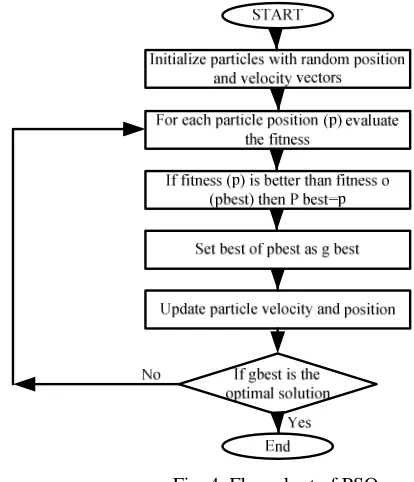
There are so many researchers who developed the techniques to tune the parameters of controllers. In this paper we are using PSO technique to optimize the parameters of controller. The flow chart of PSO is given below.
Fig. 4. Flow chart of PSO
Tuning of the parameters takes place to tune the parameters of controllers and the tuning gives the parameters of the controllers given in the table 1.
Table 1. Optimized value of parameters of P, PI and PID controller
Controller
Optimized parameters
KP KI KD
P 0.24 - -
PI 0.26 0.30 -
PID 0.1158 0.2956 0.1145
[image:3.595.315.522.223.464.2]
4. SIMULATION AND RESULTS
Fig. 5. SIMULINK model of Electro-hydraulic servo control system
The model of EHSS is simulated with the help of MATLAB/SIMULINK. The simulink model of the system is given in figure 5. Step signal is used as the reference signal. The optimized values of the parameters are simulated with the help of simulink model.
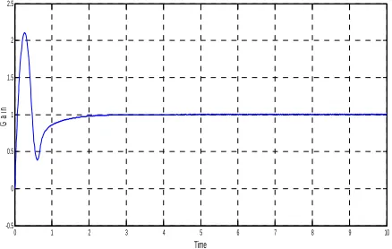
The response curve of system for P, PI and PID controllers are given below
0 1 2 3 4 5 6 7 8 9 10
-0.5 0 0.5 1 1.5 2 2.5 3
Time
G
a
[image:4.595.42.285.114.205.2]in
Fig. 6. Response curve of system using P controller
0 1 2 3 4 5 6 7 8 9 10
-0.5 0 0.5 1 1.5 2 2.5
Time
G
a
in
[image:4.595.301.564.321.385.2]Fig. 7 Response curve of system using PI controller
Fig. 8. Response of the system using PID controller
Table 2. Settling time and peak amplitude of different controllers using PSO.
Controller Parameters of controller Settling Time (sec) Peak Gain
P 1.1 2.65
PI 2.5 2.1
PID 4.8 1.35
The table 2 gives the settling time and peak amplitude gain of different controllers. Settling time of P controller and PI controller is lesser than PID controller but the peak gain of the P controller and PI controller is more than the PID controller. This gain is too high which is not be acceptable. This much of high gain will damage the component used in the system. So by using P controller and PI controller the system will not perform good. A compromising value of settling time and peak gain is required which will not affect stability. So here we can see that in the case of PID controller the settling time is of compromising value and the peak gain is also not very high.
5.CONCLUSION
[image:4.595.58.286.345.475.2] [image:4.595.77.296.522.661.2]REFERENCES
[1] Noah Manring, “Hydraulic Control Systems”, John Wiley & Sons Inc, New york, 2005.
[2] John watton, “Fundamental of Fluid Power Control”, Prentice Hall, New Jersey, 2009.
[3] Jianyong Yao, Zongxia Jiao, Bin Yao, “High bandwidth aduptive robust control for hydraulic rotary actuator”, International conference on Fluid Power Mechatronics (ICFPM), pp. 81-85, Augest 2011.
[4] Ayman A. Aly, “Velocity feedback control of a mechatronics system”, I. J. Intelligent Systems and Applications, vol. 8, pp. 40-46, July 2013.
[5] R. F. Fung and R. T. Yang, “Application of variable structure controller in position control of a nonlinear electrohydraulic servo system”, Computers & Structures, vol. 66, no. 4, pp. 365-372, 1998.
[6] Mark Karpenko, Nariman Sepehri, “On quantitative feedback design for robust position control of hydraulic actuators”, control Engineering Practice, vol. 18, pp. 289-299, Issue 3, March 2010.
[7] A. A. Aly, “Modeling and control of an electro-hydraulic servo motor applying velocity feedback control strategy”, International Mechanical Engineering Conference, IMEC2004, Kuwait, 2004.
[8] Hideki Yanada, Kazumasa Furuta, “Adaptive control of an electrohydraulic servo system utilizing online estimate of its natural frequency”, Mechatronics, vol. 17, issue 6, pp. 337-343, April 2007.
[9] Mehdi Nasri, Hossein Nezamabadi-pour and Malihe Maghfoori "A PSO based optimum design of PID controller for a linear brushless DC motor", World Academy of Science, Engineering and Technology 26 2007.
[10]C. Coon, “Theoretical Consideration of Retarded Control,” Transactions of the ASME, Vol. 75, 1952, pp. 827-834.
[11]H. E. Merrit, “Hydraulic Control Systems”, John Wiley & Sons Inc, New York, 1967.
![Fig. 2. Diagram of MOOG poition control valve [11].](https://thumb-us.123doks.com/thumbv2/123dok_us/745656.1085226/2.595.308.517.219.457/fig-diagram-moog-poition-control-valve.webp)