1 Abstract— The quantum Rayleigh spontaneous emission replaces entangled photons with independent ones in homogeneous dielectric media where single photons cannot propagate in a straight line. Single and independent groups of photons, described by the original bare states of Jaynes-Cummings model, deliver the correct expectation values for the number of photons carried by a photonic wavefront, its complex optical field, and phase quadratures. The intrinsic longitudinal field profile associated with a photonic wavefront is derived for any instantaneous number of photons. These photonic properties enable a step-by-step analysis of various beam splitters and interferometric filters. As a result, generalized expressions are derived for the correlation functions characterizing counting of coincident numbers of photons for fourth-order interference, whether classical or quantum optical, without entangled photons.
Index Terms— Quantum Rayleigh emissions, photonic beam splitters and filters, photon coincidence counting, HOM dip with no entangled photons.
I. INTRODUCTION
ECENT developments in the integration of photonic devices for quantum information processing [1-2] are characterized by their capability to generate two-photon destructive interference for temporally overlapping indistinguishable photons, which is commonly known as the Hong-Ou-Mandel dip [3]. The reduction in the counting rate of coincident detection of photons at two spatially separated photodetectors is explained by opposite sign amplitudes for the probabilities of detecting each photon pair after having been reflected or transmitted by a beam splitter. Yet, with only one pair of photons present in the experimental setup, at any given time, the two types of detection cannot take place simultaneously.
In a 1999 review paper [3], Mandel wrote: “…about the quantum state of a system: in an experiment the state reflects not what is actually known about the system, but rather what is knowable, in principle, with the help of auxiliary measurements that do not disturb the original experiment. By focusing on what is knowable in principle, and treating what is known as largely irrelevant, one completely avoids the anthropomorphism and any reference to consciousness that some physicists have tried to inject into quantum mechanics.“ [1, p. S279]. But on the next page of [3, Sect. VI] the following statement appears: “Let us consider the quantum state ∣ Ψ 〉 of the photon pair emerging from the beam splitter (BS). With two photons impinging on
A. Vatarescu is with Fibre-Optic Transmission of Canberra, 32 Batman Street, Canberra, ACT Australia. ( e-mail: [email protected]).
the BS from opposite sides there are really only three possibilities for the light leaving BS: (a) one photon emerges from each of the outputs 1 and 2; (b) two photons emerge from output 1 and none emerges from output 2; (c) two photons emerge from output 2 and none emerges from output 1. The quantum state of the beam-splitter output is actually a linear superposition of all three possibilities in the form ∣Ψ〉= ( |R |2 –
| T | 2 ) ∣ 1 〉
1∣ 1 〉2 + √2 i (| R T |2 [ ∣ 2 〉 1∣ 0 〉2 + ∣ 0 〉 1∣ 2 〉2 ]
where R and T are the complex beam-splitter reflectivity and transmissivity.” But, the possibility of other physical processes is ignored.
The assumptions made in relation to an optical beam splitter – operating in the quantum regime – would have the total number of photons entering the beam splitter input ports equal the number of photons emerging from the two output ports, leading to a unitary transformation for the input-output relation [4] of the field operators and a ± π/2 phase difference between the coefficients R and T.
However, in line with the concept of knowable elements of the experimental configuration suggested by Mandel [3], the quantum Rayleigh conversion of photons [5-7] may give rise to additional output states: ∣0〉 1∣0〉2, ∣1〉 1∣0〉2 , and ∣ 0 〉 1∣ 1 〉2
as photons are absorbed and spontaneously re-emitted, randomly, and, most likely, not in the direction of interest [5-7]. The Hamiltonian of interaction between the electric dipoles and the optical field is [5]:
𝐻̂ = 𝜅 ( 𝑑̂†∙ 𝑎̂ + 𝑑̂ ∙ 𝑎̂†) (1)
where 𝑑̂ is the electric dipole operator raising the atomic electron from one level to the next, and 𝑎̂ is the photon annihilation operator, with 𝑎̂† its conjugate operator, the photon creation operator. The optically linear susceptibility χ(1) is
included in the spatial coupling coefficient κ.
The absorption of one photon through quantum Rayleigh conversion leads to the disappearance of an entangled state, that is: 𝑎̂1( ∣ 0 〉 1∣ 0 〉 2 + ∣ 1 〉 1∣ 1 〉 2) = ∣ 0 〉 1∣ 1 〉 2 which is a product state. A similar annihilation occurs for the second photon. Alternatively, the dipole-field interaction of absorption projects the state onto the zero-photon state: 1〈 0 ∣𝑎̂1∣1〉 1∣1〉 2
= ∣ 1 〉 2 , resulting in one single photon surviving as soon as
the entangled pair was created in a parametric spontaneously down-converted emission in an optically nonlinear crystal. Additionally, unless two state functions or relevant operators overlap in the space-time of their configuration, i. e. f 1(r, t) ≠
0 and f 2 (r, t) ≠ 0, their product will be zero [5].
The Quantum Regime Operation of Beam
Splitters and Interference Filters
Andre Vatarescu
In a nonlinear crystal pumped, e.g., with a continuous wave (cw) and for frequency down-converted photons of ω s + ω i =
ωp , the gain providing medium generating the spontaneous
emission, will also amplify the initially single photons, particularly so in the direction of wavevector matching conditions. As a result, the commonly assumed one single photon output does not, in reality, physically happen. At least several photons will be associated with each individual and discrete electronic “click”.
Based on the analysis of [5], with the Fresnel formulas for the optical reflection and transmission coefficients corresponding to probability amplitudes of the two events, the photonic conservation would apply only to one interface between two dielectric media. As additional internal reflections inside the glass plate of a beam splitter would take place, the assumption of photon number conservation is questionable. Furthermore, because of the quantum Rayleigh conversion or coupling of photons occurring inside a dielectric medium [8], one single photon can only be re-emitted spontaneously in a random direction, preventing a straight line propagation. Only a group of photons propagating together can maintain their direction of propagation and characteristics through stimulated emission induced by the other photons which are not temporarily absorbed and re-emitted.
We can apply the Fresnel formulas if a pure state vector, or wavefunction, can be identified for the optical field – measured instantaneously [9-10] – of the time-varying photonic wavefront, i.e., its amplitude in terms of the flux of photons and its phase. Such a function is developed in Section II below, taking the form of | Ψn〉 = ( | n 〉 + | n −1〉) / √ 2 and delivering,
classically compatible, c - number values for observable expectation values [11].
A pure state delivers one single measurement [9], [12] whereas a mixed state describes the statistical distribution of an ensemble of measurements [12]. A photonic wavefront carries a number of photons across a plane hosting dipoles and its duration will be determined by the response time of the photon-dipole interaction [9].
The physical process of quantum Rayleigh conversion of photons (QRCP) is associated with the real part of the first-order optical susceptibility and involves a group of electric dipoles interacting simultaneously with two photonic wavefronts carrying an arbitrary number of photons across a plane over a short time ∆ t → 0. The excited dipoles will emit either spontaneously or stimulatedly, depending on the circumstances. The spontaneous emission will affect the operation of dielectric interface-based beam splitters, while the stimulated emission will be active in a fiber-optic beam splitter configured as an optical directional coupler.
A mixed state of one-photon excitation as presented in [13, p. 8] is impractical for the description of the QRCP because the photon wave packet |1⟩j ,σ describes an output-measured spatial-
and temporal-localized packet. “An example is the deterministic generation of a single photon from an atom in a cavity-QED system. If the packet is dispersed spectrally by a prism and detected by an array of photon counters, only one counter will click, although which one clicks will be random. Such a state is expressed as |1⟩j, σ =∫ 𝑑3𝑘 𝑈𝑗
(𝜎)
(k)|1⟩k,σ /(2 𝜋)−3
where |1 ⟩j ,σ is a state with a single excitation having particular
monochromatic wave vector-polarization state labeled by the pair (k, σ). We see that the function 𝑈𝑗(𝜎)(k) fully specifies the state.” [13, p. 8] This state is of no utility for evaluating the optical field involved in a dipole-photon interaction as the expectation values vanish, i.e., j ,σ⟨ 1 |â|1 ⟩j ,σ = 0. For the
single-photon wave packet, only one radiation mode is taking part in the detection or photon coupling processes. Yet, an intrinsic photonic field distribution is carried by each interacting photon without any dependence on the measured statistical distribution of the ensemble of the mixed state.
The interactions associated with quantum Rayleigh conversions of photons require a wavefunction capable of delivering transient or instantaneous expectation values for a pure state. This is presented in Section II, and followed by the description of the intrinsic photonic field profile in Section III. These elements will underpin the analysis of various types of beam splitters, and interference filters in Section IV. Physical aspects of the dynamic and coherent number states are discussed in Section V along with the irrelevance of photonic entanglement to explain previously published experimental results.
II. PHOTONIC WAVEFRONT EXPECTATION VALUES AND DYNAMIC MOTION
As the number of photons and related field amplitude and phase carried by a photonic wavefront may change as a result of the QRCP, the equations of motions for the corresponding expectation values will be evaluated with the Ehrenfest’s theorem [14-15]. To this end, a pure quantum state is needed, capable of delivering correct values for the instantaneous number of photons, the optical field amplitude and its longitudinal profile and the phase quadratures.
Photons and their instantaneous properties are detected and measured as a sequence of wavefront number states | n 〉 [9]
which make up a pure quantum state vector | Ψ ( r, t ) 〉 = ∑ n c n ( r, t ) | n 〉 regardless of the overall distribution to
which the photons belong [9-10]. The quantum probability of occupation of an eigenstate is given by the normalized distribution of photons – crossing a surface at location r –with
the time-varying coefficients | cn | 2 satisfying the condition
∑n| cn |2 = 1, and orthogonality 〈 n | m〉 = δ n m . The detection
of photons occurs as a result of their optical field exchanging energy with electrons of the atomic structure of the detector, similarly to the Jaynes - Cummings model [4], [14] for the quantized dipole-photon exchange of energy. The detection, or any other interaction process, collapses the photonic quantum state into an instantaneous eigenvalue of a number operator [15] regardless of the ensemble distribution to which it belongs, e.g., a coherent state or an arbitrary distribution.
A. Optical fields of dynamic and coherent number states
Based on the formalism presented in [5], [16], the magnitude of the Poynting vector, i.e. the flux of energy E ( or number of photons /s ) carried by an optical wavefront of frequency ω and crossing a plane surface at position z is given in terms of the electromagnetic field magnitudes E and B , or corresponding operators, by the equalities: E = ω ε E 2+ c2 ω B 2 = 0.5 ħ ∙ ω (a a* + a* a ) (2)
3 with a = ( ε / ħ ) ½ ( E + i c B ) and its complex conjugate a* .
From this relation one defines the annihilation and creation operators as:
â =( ε / ħ ) ½ (Eˆ +
i
c
Bˆ) (3a) â †= ( ε / ħ )
½(
Eˆ–
i
c
Bˆ) (3b)
with ε and ℏ indicating the permittivity of the medium and the reduced Planck constant, respectively. The free-space Hamiltonian
f
Hˆ is explicitly written as [5]:
𝐻̂𝑓 = ħ ∙ ω 𝑁̂𝑐 (4a)
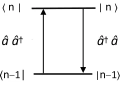
𝑁̂𝑐 = 0.5 ( ↠â + â ↠) (4b)
where 𝑁̂𝑐 is a complete number operator and its eigenstates are the number states | n 〉. The field operators â and its adjoint ↠connect
〈
n
||
n
〉â â
†â
†â
〈
n
−1
|
|
n
−1
〉Fig. 1. An illustration of the dynamic and coherent two-component number states.
We note that: 〈n | ↠= √n〈n−1| , and 〈n−1| â = √n〈n | .
two consecutive number states, and consequently, a superposition of | n −1〉 and | n 〉 should give rise to a non-zero optical field for the following state vector:
| Ψ n (t) 〉 = c 1 (t) | n 〉 + c 2 (t) | n− 1〉 (5a)
| Ψ n〉 = 2 – 1/2 ( | n 〉 + | n− 1〉 ) (5b)
with the normalization of | c 1 | 2 + | c 2 | 2 = 1 .
Analogously to the derivation [4] of coherent states of light | α 〉, the non-Hermiticity of the photon annihilation and creation operators allows for complex classical numbers ( c –numbers) to be delivered when these operators act on number states. Applying â and ↠to | n 〉 returns a complex c – number
s n = | s n | exp (− i φ n ) (6)
which will become the complex amplitude of the state, so that:
â | n 〉 = s n | n −1 〉 (7a)
↠| n− 1〉 = s *n | n 〉 (7b)
Recalling that â and â†are adjoint operators of each other, they
interchange roles when acting on the Hermitian conjugate ( or bra) wave functions:
〈 n −1| â = s n 〈 n | (8a)
〈 n | ↠= s *n 〈 n − 1 | (8b)
The condition of the number states being eigenstates of the number operator 𝑁̂ = ↠â requires that | s n | 2 = n .
This symmetric Hamiltonian of (4) suggests the two-component state vector of (5) as depicted in Fig. 1, and it carries out two simultaneous operations, one as a two-step number operator
〈 n | ↠â | n 〉= 〈 n | ↠| n − 1 〉 s n = 〈 n | n 〉 s n s*n (9)
and the second operation – illustrated in Fig. 1 – as a one-step transition operator between two consecutive number states, each operator acting on the state vector next to it (or the left-hand operators acting on the Hermitian conjugate wave functions 〈 n | , the result being:
〈 n | ↠∙ â | n〉 = s *n 〈 n −1 | n −1〉 s n = | s n | 2 = n (10a)
〈 n −1| â ∙ ↠| n −1〉 = s *n 〈 n | n 〉 s n = | s n | 2 = n (10b)
We point out that for │ Ψn〉 from (5b) one obtains
〈 Ψn │ ↠â │ Ψn〉 = 0.5 ( n + n − 1 ) = n – ½ and
〈 Ψn │ â ↠│ Ψn〉 = 0.5 ( n + n + 1 ) = n + ½ , leading to
〈 Ψn │ 𝑁̂𝑐│ Ψn〉 = 0.5 x 2 n = n ( 11)
which is the number of photon carried by the wavefront flux. In the Heisenberg picture, the propagating photon field operators take the form [5]:
â (ω , t, z) = â (ω) f (x , y, z )
e
−i ( ω t − β z )(12a)
↠(ω, t, z) = ↠(ω) f (x , y, z )e
i ( ω t − β z )(12b)
where the spatial distribution is a solution of the Helmholtz wave equation [5] . The observable quantity of the expectation value of the quadrature field operator 𝑄̂ = â + ↠is found by combining (5b) ,(6), (7), (8) and (12) to yield:
〈 Ψn ( t )│
â
│Ψn ( t ) 〉 = 0.5e
−i ( ω t + φ (0) ) n 1 / 2e
− i φ n(13a)
〈 Ψn │( â + ↠)│ Ψn〉 = n ½ cos (ω t − β z − φ n ) (13b)
reproducing the c - number 〈𝑄̂〉corresponding to the “classical” optical field with a time-varying number of photons n (t) and related phase φ n (t) .
The correct expectation values can also be found for the quadrature operators [17], i.e., 𝐶̂ = 𝑎 ̂ 𝑁̂−1/2 + 𝑁̂−1/2 𝑎̂† and 𝑆̂ = 𝑖 (𝑎 ̂ 𝑁̂−1/2 − 𝑁̂−1/2 𝑎̂† ) :
〈 Ψn │𝐶̂𝑗│ Ψn〉 = cos (ω t + φ j ) (14a)
〈 Ψn │𝑆̂𝑗 │Ψn 〉 = sin (ω t + φ j ) (14b)
B. The equations of motion of the optically linear parametric
interactions.
the simultaneous presence of another beam of photons of the same frequency. This effect is described by the Ehrenfest theorem [15]:
𝑖 ℏ 𝜕
𝜕𝑡 〈 Ψ𝑛 (𝑡)| 𝑎̂ | Ψ𝑛 (𝑡)〉 =
= 〈 Ψ𝑛 (𝑡)| [ 𝑎̂ , 𝐻̂𝑖𝑛𝑡 ] | Ψ𝑛 (𝑡)〉 (15) indicating that the expectation value of the optical field is modified by its commutator with the Hamiltonian of interaction 𝐻̂𝑖𝑛𝑡 .
Having identified a quantum wave function capable of delivering the instantaneous magnitude and phase of an optical field, we can now apply the formalism of [18-19] to the propagation along an optical waveguide directional coupler by employing the following composite photonic quantum state function │Φ〉 for two optical waves identified by their waveguide, their Hamiltonian of interaction and the equation of motion derived from (15):
│Φ 〉 = │Ψn, 1〉 │Ψn, 2〉 (16)
𝐻̂𝑖𝑛𝑡 = ℏ 𝜔 𝜒(1) (𝑎̂2
†
𝑎̂1+ 𝑎̂2 𝑎̂1 †
) (17)
𝜕
𝜕 𝑡〈 Φ | 𝑎̂1 | Φ〉 = −𝑖ω𝜒
(1) 〈 Φ | 𝑎̂
2 | Φ〉 (18) where χ(1) is the real part of the first-order susceptibility of the
dielectric medium. This interaction will modify the complex field amplitude sn , j (j = 1 , 2) of two co-propagating and
overlapping optical beams of the same frequency, identifiable by their respective optical waveguides (j = 1 , 2) . From. (13) we have for the expectation values of the optical fields
〈 Φ │ â j│ Φ 〉 = 0.5
e
−i ( ω t + φj (0) ) s n, j (19)After converting to number of photons, i.e., | sn , j | 2 = N j
and corresponding phases φ j , the equation of motion (18)
provides the rates of change of N j and φ j as follows
[18-19]: 𝜕
𝜕 𝑧 𝑁1= 𝑔1 𝑁1 (20a)
𝑔
1= − 𝜅 (
𝑁2 𝑁1)
1/2
𝑠𝑖𝑛 𝜃
21(20b)
𝜕
𝜕 𝑧
𝜃
21= (𝛽
2− 𝛽
1)
+
𝜅 [(
𝑁1𝑁2
)
1/2
− (
𝑁2𝑁1
)
1/2
] 𝑐𝑜𝑠 𝜃
21(20c)
𝜕
𝜕 𝑧
𝜑
1=
𝜅 (
𝑁2 𝑁1)
1/2
𝑐𝑜𝑠 𝜃
21(20d)
𝜅 =
𝑘02 𝑛
∫ ∫ 𝑑𝑥 𝑑𝑦 𝜒
(1)𝑓
1
𝑓
2𝒆
𝟏∙ 𝒆
𝟐(20e)
where the gain coefficient
𝑔
includes an overall coupling coefficient κ defined in [8] which depends on the polarization states e1 and e2 of the photons. The phase difference betweenthe two waves is θ 2 1 = ( β 2 − β 1 ) z + φ 2 − φ 1 , β being
the propagation constant and z / t = v p is the phase velocity. In (20e)
k o and n specify the free-space wavevector and the effective refractive
index, respectively. It should be noted that equations (20) describe the physically meaningful process of quantum Rayleigh conversion of photons [8]. The coupling coefficient of Eq. (20e) indicates that the entire local value of the optically linear susceptibility χ (1)
is involved
in the coupling process in the dielectric medium at any point where the two spatial distributions f1 and f2 overlap, each having units of m –1,
and the squares f 2 are normalized to a dimensionless unit over the
cross-section area. This is in contrast to the physically impossible coupling between two optical waveguides apparently induced by a perturbation of the dielectric constant in the cladding – see reference [8] for details.
Two dynamic number states of (16) co-propagating through a dielectric medium will couple photons from one state to the other depending on the relative phase between the two waves. This process, repeatedly, will eliminate optical waves whose phases diverge substantially from the phase of the surviving wave which will dominate the output of a lasing cavity.
Two groups of photons propagating simultaneously across the same dielectric medium would exchange photons, parametrically, with each other through the real part of the susceptibility – see (20) above – which is indicative of a beam splitter composed of a fiber-optic directional coupler [1-2].
C. Interference patterns between the fields of dynamic and
coherent number states
Another useful effect is the interference between two waves reaching a photodetector. In the context of this analysis, one obtains that, in so far as localized detection of photons of two dynamic and coherent number states is concerned, the photocurrent I p h generated by the
interference output of a balanced homodyne detector is calculated by combining the expectation values of the quadrature field operators given in (13) to obtain:
〈 I p h ( t ) 〉= K ( 〈 Q 1〉+ 〈 Q 2〉 ) 2 =
= K [ Ν 1 cos 2 (ξ1 ) + Ν 2 cos 2 (ξ2 ) +
+ 2 ( Ν 1 Ν 2 ) 1/ 2 cos (ξ1 ) cos (ξ2 ) ] (21)
with the constant of proportionality K corresponding to the quantum efficiency of photon – to – electron conversion. The phases are defined by ξ j = ω j t − β j z − φ j . This approach of making use of initially
evaluated expectation values links the quantum regime to the classical one [20]. After time-averaging over a large number of optical frequency periods, namely, with the averaging time interval T satisfying 2 π / ω j << T << 2 π / | ω 1 - ω 2 ) | we find that 〈cos 2 (ξ) 〉 = 1/ 2 and 〈cos (ξ1 + ξ2 )〉 = 0, as well as 〈sin ξ〉= 0, to retrieve the
conventional interference pattern: 〈 I p h ( t ) 〉= ( K / 2) [ Ν 1 + Ν 2 +
+ 2 ( Ν 1 Ν 2 ) 1/ 2 cos (ξ1 − ξ2 ) ] (22)
5 power and any related phase. The question of measured variances induced by system fluctuations will be addressed in Section V below.
III. INTRINSIC FIELD PROFILE OF A PHOTONIC WAVEFRONT We can calculate the intrinsic longitudinal field profile of a group of photons, or its coherence length, by using the wave function │Ψn 〉
from (5b). Two equations can be identified for the expectation values of â, or the corresponding c - numbers, by combining (3) and (13a), leading to:
〈 Ψn│ â │Ψ n 〉 = b 〈 𝛦̂ 〉 + i s 〈 𝛣̂ 〉 (23a)
〈 Ψn │ â │ Ψn 〉 = q
e
−i ω t(23b)
where q = 0.5 √ n , b = (ε / ℏ ) 1 / 2 and, s = (ε c / ℏ ) 1 / 2 . We point
out that both quadratures of the field are represented in the phasor notation of (23). Eq. (23a) is obtained from (3) and can be expressed in terms of the c – numbers E = 〈 𝛦̂ 〉 and B = 〈 𝛣̂ 〉. Recalling the relations [16] between the vector potential A ( z , t ) and the fields as:
E =− ∂ A / ∂ t and B = xA (24) in the Cartesian frame of coordinates ( x , y , z ), the vectors have the
notation, in the plane wave approximation: A = ( A , 0 , 0 ) ; E = ( E , 0 , 0 ) ; B = ( 0 , B , 0 ) and the wave vector is
k = ( i k x
, i k
y, β ) for a beam propagating in the z – direction in an
optical waveguide. The complex amplitude of the vector potential is represented by
A
( z, t ) =A
p ( z ) f (x , y)e
−i ( ω t − β z ) (25)
where the lateral profile of the guided mode is given by f ( x , y) and the propagation constant by β = 2 π n eff / λ . The second term of the
curl operation x f (x , y) x = ( ∂ f / ∂ z
)
y − ( ∂ f / ∂y
)
zdoes
not lead to wave propagation and does not affect measurements in a plane perpendicular to the z - coordinate. The second term will therefore be set aside in the remainder of this analytic derivation.
Relating
Α
pto a moving source of photons would suggest a
relative distance ζ = z − z o with z o being the temporal location of
the photons and the localization given by a Dirac delta function δ ( z− z o ) , resulting in this differential equation after substituting
(24) and (25) into (23) multiplied by the propagation phase exp i (β z ) of the annihilation operator :
𝜕
𝜕 𝑧𝐴𝑝 + 𝜎𝐴𝑝 = 𝛾 𝛿( 𝑧 − 𝑧𝑜) (26) where σ = b ω / s + i β = ( ω / c ) ( 1 + i n eff ) , and γ =−i q / s
= i 0.5 (n ℏ / ε ) 1/2 . Setting A
p ( z ) = g ( z ) e –σ z and
inserting into the differential equation (26) leads to:
∫
d g = = γ∫
e
σ z δ ( z − zo ) d z . With g
= γ
e
σ z o,
and for reasonsof physical symmetry, the longitudinal distribution of
the magnitude
of the vector potential associated with photons of a wavefront isfound to be:
A p( z ) = γ e– σ | z − zo | (27)
The vector potential’s decay constant is inversely proportional to the wavelength λ through Re σ = 2 π / λ . Thus, the local optical field includes contributions from photons in the vicinity of z o , as
illustrated in Fig. 2. The longitudinal optical field profile g f of
one photon of wavelength λ , crossing point zo , is obtained from
(27) to be:
g f ( z = c t ) = exp
(– 2 π | z
− zo| / λ ) (28)which has the form of a Wigner spectral component S (ω, t), that is, a time-varying spectral component [21] – as opposed to a time-constant amplitude and phase of a Fourier spectrum – crossing a surface perpendicular to the wavevector of propagation. The exponential decay of the spatio-temporal profile is identical to that obtained by Fourier transforming a fully populated transmission line of an interference filter [10].
Fig. 2 Partially overlapping photon
fields.
The coupling coefficient of (20e) will be modified below so as to take into account the longitudinal profile of the optical field given in (28) – which is, in fact, its intrinsic physical coherence length – for the operation, as a beam splitter, by an optical fiber directional coupler.
IV. THE BEAM SPLITTERS AND INTERFERENCE FILTERS The quantum regime of photonic interference would involve only one photon per radiation mode [3]. Yet, as pointed out in the Introduction, one single photon propagating by itself, in a dielectric medium, will not follow a straight line inside a dielectric medium because of the quantum Rayleigh spontaneous emission [5-7]. Only a group of monochromatic photons propagating together can maintain a straight line of propagation as a photon absorbed by an electric dipole will be immediately recaptured through stimulated emission by the other photons in the group.
The appearance of temporarily discrete groups of photons in the process of parametric down-conversion is due to the unavoidable amplification of spontaneously emitted photons, particularly so, in the phase-matching direction. Such optical signals are best described by means of the mixed time-frequency (or Wigner-type) spectrum [21], with the time-frequency amplitude itself being a function of time, i. e. , S (ω , t ) specifying, in other words, a time-varying number of monochromatic photons being carried simultaneously by a photonic wavefront.
by a photonic wavefront and its associated complex amplitude in (13). Equally, the optical field profile of a group of photons is shown in (27) to be independent of the type of source that emitted them, cf. [13]
Given a photonic optical field, the Fresnel coefficients of reflection and transmission can be interpreted as probability amplitudes for the respective effects at a dielectric boundary [5]. At least three types of beam splitters can be identified: the glass plate of Fig. 3, the cubic prism of Fig 4, and the optical waveguide directional coupler composed of optical fibers [1-2]. Their operations involve the quantum Rayleigh spontaneous and stimulated emissions.
A. The Glass Plate Beam Splitters and the HOM dip
For a plate beam splitter sketched in Fig. 3, the primary reflected and transmitted optical fields will lead to the transformation:
â†c = − r 01 â†a + t01 t10
â†b (29a)
â†d = t01 t10
â†a + t01r10t10 â†b (29b) where the subscripts of the reflection r and transmission coefficients t indicate the boundary interface, with the first subscript corresponding to the incoming direction of the photons.
To illustrate an application of this approach, two groups of photons generated as the signal (s) and idler (i) waves in a parametric down-conversion of a cw optical pump are impinging, from opposite sides, on a glass plate operating as an optical beam splitter which is placed in the xy plane. With the upper boundary used as the synchronization place for the two
groups, i.e. τ = 0, the output field operators are:
𝑎̂𝑐= − 𝑟𝑠 𝑎̂𝑠 + 𝑡𝑖 𝑎̂𝑖and, 𝑎̂𝑑= 𝑡𝑠𝑎̂𝑠 + 𝑟𝑖 𝑎̂𝑖 , with reflection (r) and transmission (t) coefficients identified by the type of photons. The relative phases of these photonic wave fronts are:
a
c
n
o
n
1n
1 >n
0n
ob d
Fig. 3. A typical glass plate beam splitter. Photons arrive simultaneously at the upper dielectric boundary.
θ s r (τ) = −ω τ + φ s (t)−π (30a) θ i t (τ)
=
φ i(t)+γ (30b) θ s t (τ) = φ s (t) +γ
(30c) θ i r (τ)
=
ω τ + φ i ( t) +2γ (30d)
where the random phases of the spontaneously emitted photons are denoted by φ (t)and γ is the phase added during one transit
propagation between the boundaries of the BS and a (−π) phase shift is due to the upwards reflection. Moving the BS in the
z-direction will bring about a time delay ±τ between the two wavefronts reaching the same photodetector. The number of photons N j (t) detected by photodetector j =1; 2 is evaluated
from the interference pattern of the instantaneously measured flux of photons presented above in (22):
N j ( t ) = K [ Ns j ( t ) + Ni j ( t ) +
+ 2 [Ns j (t) Nij (t)] 1/2 cos[(θ (t ) s j − θ ( t ) i j )] (31)
where the phases are given by (30a-d), e. g., θ (t) s1 = θ s r (τ)
and θ ( t ) i 1 =θ i t (t , τ). The correlation function
C12 (τ) = 〈 N1 ( t
)
N 2( t + τ ) 〉 (32)of coincidence counting of photons for the transient interference patterns of the two separate photodetector intensities, over the coincidence time interval T (a few ns) is derived to be:
C12 (τ) = No1 No 2 [ 1 + σ 1 σ 2 Γ1 Γ2 cos Θ ] (33 )
where σ j = 2 ( Njs N j i ) 1/2
/ (N
js + N j i ) for photodetectorj = 1 or 2, and the overlap integral
Γj (τ) = 0 g f (t) g f ( t +τj ) d t
/
0 g f 2 (t) dtis normalized. With the phase difference Θ for the intensity correlation given by
Θ = [θ s r − θ i t ] − θ s t −θ i r] = (ωi −ωs)
τ
− π ()there are two statistical possibilities for the random phases φ s
andφ i of the spontaneously emitted photons. These two
random phases can interchange values without affecting the result, and the cosine term 0.5 cos Θ should be counted twice when calculating, “classically”, the correlation function C12 (τ).
From (34), Θ = −π for τ = 0, and with equal numbers of photons in the interfering waves, so that, σ 1 = σ 2 = 1, we find
from (33) a vanishing correlation C12 (0) = 0 , which
corresponds to the Hong–Ou–Mandel dip [22-23].
Therefore, there is no need for entangled photons to explain the coincidence counting of photons by two separate photodetectors. The only requirement is that the two groups of photons are split between the two detectors and are synchronized at a chosen interface.
Other combinations of the relative phases Θ are possible by setting up a Mach-Zehnder interferometer configuration with two identical 50:50 beam splitters, placing one at the input and the other at the output of the interferometer [24]. Basically, there are four waves or groups of photons reaching each of the two photodetectors. We will denote them as s1 for the unmodulated signal wave and s2 for the modulated signal wave, and as i1 for the unmodulated idler wave and i2 for the modulated idler wave.
Next we choose, for degenerate frequencies of the signal and idler waves, the interference term cos (−ω τ + φ s1− φ s2 )
from one of the detectors and the cos (−ω τ + φ i1− φ i 2 ) term
7 phases of weak waves, with the coherent phase of the pump photons given by φ p. All this leads to the average value of the
fourth-order numerical interference:
〈cos (
−
ω τ + φ s1−
φ s2) cos (−
ω τ + φ i1−
φ i 2 ) 〉 == cos (
−
2 ω τ )(35) which oscillates with the pump frequency [24]. Similar expectation values may be derived for any combination of any two interference patterns, one from each photodetector, e.g. [24-26]. It is noteworthy that the phases of the spontaneously emitted photons do not appear in the conventional quantum descriptions of two-photon beats, e.g. [22-26].
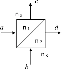
B. The Cubic Prism Beam Splitter
For a cubic beam splitter made up of two butting prisms of different refractive indexes as sketched in Fig. 4, the field transformation becomes:
â
†c=
−
t
01r
12t
10â
†a +t
01t
12t
10â
† b (36a)â
†d=
t
01t
12t
20â
†a +t
02r
21t
20â
† b (36b)The subscript 0 indicates free space, and subscripts 1 and 2 refer to the refractive index of each of the two prisms.
In the case of the cubic prism BS, any two external surfaces can form a resonant cavity through reflection or transmission at the diagonal interface. The output states will be affected by photons temporarily trapped inside the BS, leading to the possibility of additional quantum states, as well as quantum Rayleigh coupling of photons – see (20) .
c
n
o
a
n
1d
n
2
n
ob
Fig. 4. A typical cubic prism beam splitter. Photons
arrive simultaneously at the diagonal boundary interface
. n
2 >n
1 >n
0C. The Fiber-optic Beam Splitter
The longitudinal optical field profile of a group of monochromatic photons was derived in (28) and has the form of a Wigner spectral component S (ω, t ), that is, a time-varying spectral component [21] – as opposed to a time-constant amplitude and phase of a Fourier spectrum – crossing a surface perpendicular to the wavevector of propagation.
For the optical directional coupler, the evolution of the photons is governed by Eqs. (20) with the possibility of one waveguide capturing most of the photons resulting in an asymmetric output. The coupling coefficient κ will have to take into consideration the temporarily discrete nature of the groups
of photons by including the longitudinal field profile g f (z) next
to the transverse spatial field f, that is:
𝜅 =
𝑘
02 𝑛
Γ
12(𝑧
𝑜) ∬ 𝑑𝑥 𝑑𝑦 𝜒
(1)𝑓
1
𝑓
2𝒆
𝟏∙ 𝒆
𝟐(37) Γ12 (
z
o) =∫
dz g f (z – z o 1) g f (z – z o 2)This spatio-temporal overlap is characteristic of the quantum regime of discrete groups of photons. The phase-dependent coupling of photons of (20) is critical in the operation of the optical fiber beam splitters by creating, with the adjustable phase difference, an asymmetric output [25-26].
Future integration of photonic components will replace the optical fiber splitter with integrated waveguides.
D. The Interference Filter
Experimental configurations for two-photon quantum beats, e.g. [22-26], employ interference filters in order to control the coherence length of the photon.
The extent of the correlation fringes is determined by the coherence length of the photons, which can be shaped by an interference filter, apparently operating on the output spectral distribution Φ (ω 1 , ω 2) of the ensemble of photons generated
by an active source over a long time, such as the spontaneous parametric down-conversion mechanism [23].
However, from a physical perspective, a Fourier transform – or a superposition of spectral components – necessitates the simultaneous presence of the entire range of spectral components. But this is not the case when only one photon, at any given time, crosses an interference filter. A single monochromatic photon propagating through a Fabry-Perot type filter, or a Bragg refractive index grating in a fiber, will be delayed randomly by repeated internal reflections and will acquire an integer multiple of a bias phase or time-delay. The higher the internal reflectivity of the cavity, the longer some photons may bounce back and forth inside the cavity resulting in a “longer photon” output, which is interpreted as a longer coherence length. Such optical signals are best described by means of the mixed time-frequency (or Wigner-type) spectrum, e.g. [21] with the frequency amplitude itself being a function of time S (ω, t) specifying, in other words, a time-varying number of monochromatic photons being carried by varying photonic wavefronts. The time-stretching of the photonic group will be equivalent to pulse expansion for a narrower Fourier spectrum.
Thus, a group of photons entering, simultaneously, a resonant cavity of an interference filter, will exit at different times as the higher the internal reflectivity, the longer the time that some photons will bounce back and forth inside the cavity. This process will cause the initially bunched photons to spread out in time and give rise to a longer coherence length for photon coincidence counting as in [27]. The wavefunction describing this output would take the form:
∣ Φout ( r , t ) 〉 = Σ m c n ( r, t) f n ( r ) δ ( t − t m ) | Ψn (ω) 〉 (38) where the times t m specify the existence of a group of n photons
monochromatic and time-dependent –see (5) above, whereas the overall mixed state of the ensemble is multi-chromatic and time-independent (e.g. the bi-photon wavefunction).
The temporal profile of the optical field carried by a photon or any instantaneous photonic wavefront should be determined from a pure quantum state wavefunction because it should be unaffected by the spectral distribution of an ensemble of measurements. However, for interference to take place, at least two coefficients c n have to be non-zero.
V. PHYSICAL ASPECTS OF DYNAMIC NUMBER STATES The possibility of measuring expectation values in the context of the dynamic and coherent states of (5) raises the question of the Heisenberg uncertainty principle [15] which has to do with the joint statistical distribution of the measured values of two variables corresponding to repeated measurements of identically prepared systems [9-10], and applies to the
simultaneous measurements of two dynamic variables whose
quantum operators do not commute in a given set of state wave functions, the variables being incompatible observables [15].
The principle of uncertainty does not preclude the existence of well-defined numerical values for either variable [15]. Limited information about one variable is associated with a variance in the measured values, with more information being available about the other variable. Measurements yield precise instantaneous values – within the constraints of the equipment – by collapsing the system’s wave function into a specific value [15]. A quantum "spread" implies that measurements on identically prepared systems do not return identical results because of system-related fluctuations such as spontaneous emission, time-varying losses, temperature variations, etc.
One should not confuse prediction with measurements. It is the measured values that come into play when plotting the joint distribution of two observable, physical variables. A measurement of only one variable will still have its own variance of values but it is not subject to the Heisenberg uncertainty principle, because the physical system is not disturbed by the measurement of another variable. One can easily measure a well-defined eigenvalue of an operator [15] at a given time.
REFERENCES
[1] C. Agnesi, B. Da Lio, D. Cozzolino, L. Cardi, B. Ben Bakir, K. Hassan, A. Della Frera, A. Ruggeri, A. Giudice, G. Vallone, P. Villoresi, A. Tosi, K. Rottwitt, Y. Ding, and D. Bacco,” Hong–Ou–Mandel interference between independent III–V on silicon waveguide integrated lasers“,Opt.
Lett. Vol. 44, no. 2, pp. 271-274, 2019.
[2] H. Semenenko, P.Sibson, M. G. Thompson, and C. Erven, “Interference between independent photonic integrated devices for quantum key distribution “, Opt. Lett., vol. 44, no. 2, pp.275-278, 2019.
[3] L. Mandel, “Quantum effects in one-photon and two-photon interference,” Rev. Mod. Phys., vol. 71, pp.. S274-S282, 1999. [4] C. Garrison and R.Y. Chiao, Quantum Optics, Oxford University Press,
2008.
[5] R. J. Glauber and M. Lewenstein, “Quantum optics of dielectric media,”
Phys. Rev. A, vol. 43, pp. 467- 491, 1991.
[6] W. H. Louisell, Quantum Statistical Properties of Radiation, John Wiley & Sons, 1973.
[7] D. Marcuse, Principles of Quantum Electronics, Academic Press, 1980. [8] A. Vatarescu , “Photonic coupling between quadrature states of light in a
homogeneous and optically linear dielectric medium,” J. Opt. Soc. Am.
B, vol. 31, pp.1741–1745, 2014.
[9] G. Breitenbach, S. Schiller, and J. Mlynek, “Measurement of the quantum states of squeezed light," Nature, vol. 387, pp. 471-475, 1997. [10] A. I. Lvovsky and M. G. Raymer, “Continuous-variable optical
quantum-state tomography," Rev. Mod. Phys., vol. 81, no. 1, pp. 299-332, 2009. [11] A. Vatarescu, “Instantaneous Quantum Description of Photonic
Wavefronts for Phase-Sensitive Amplification,” Frontiers in Optics/Laser Science Conference (FiO/LS), paper JW4A.109, Washington, Sept. 2018.
[12] U. Fano, “Description of States in Quantum Mechanics by Density Matrix and Operator Techniques, ” Rev. Mod. Phys., vol. 29, pp. 74-93, 1957 [13] B. J. Smith and M G Raymer, “Photon wave functions, wave-packet
quantization of light, and coherence theory“, New J. Phys., vol. 9, 414 (2007).
[14] D. A. Steck, Quantum and Atom Optics, University of Oregon, available online at http://steck.us/teaching (revision 0.11.0, 18 August 2016). [15] D. J. Griffiths, Introduction to Quantum Mechanics, Publisher: Pearson
Prentice Hall, 2005.
[16] K. J. Blow, R. Loudon, S. J. D. Phoenix and T. J. Shepherd,”Continuum fields in quantum optics,” Phys. Rev. A, vol. 42, no. 7, pp. 4102- 4114, 1 October 1990.
[17] P. Carruthers and M. M. Nieto, “Phase and Angle Variables in Quantum Mechanics,” Rev. Mod. Phys., vol. 40, pp. 411-440, 1968.
[18] A. Vatarescu, “Photonic Quantum Noise Reduction with Low-Pump Parametric Amplifiers for Photonic Integrated Circuits”, Photonics, vol. 3, article 61, 2016.
[19] A. Vatarescu A, “Phase-Sensitive Amplification with Low Pump Power for Integrated Photonics, “OSA Advanced Photonics Congress, paper ID: IM3A.6., 2016.
[20] L. Mandel and E. Wolf, “Coherence Properties of Optical Fields,” Rev. Mod. Phys., vol. 37, pp. 231-287, 1965.
[21] L. Cohen, “Time-frequency distributions-a review,” Proc. IEEE , vol. 77, pp. 941–981, 1989.
[22] Hong, C. K., Ou, Z. Y. & Mandel, L. Measurement of subpicosecond time intervals between two photons by interference”, Phys. Rev. Lett. Vol.59, pp. 2044–2046, 1987.
[23] Z. Y. Ou and L. Mandel, “Observation of Spatial Quantum Beating with Separated Photodetectors “,” Phys. Rev. Lett., vol. 61, pp. 54 – 57, 1988. [24] M. Halder, S. Tanzilli, H. de Riedmatten, A. Beveratos, H. Zbinden, and N. Gisin, “Photon-bunching measurement after two 25-km-long optical fibers, “ Phys. Rev. A , vol. 71, 042335, 2005.
[25] H. Kim, S. M. Lee, and H. S. Moon,” Generalized quantum interference of correlated photon pairs”, Sci. Rep. vol. 5, pp. 9931-9936, 2015. [26] H. Kim, S. M. Lee and H. S. Moon, “Two-photon interference of
temporally separated photons “, Sci. Rep. vol. 6, pp. 34805-34810, 2016. [27] M.Halder, A. Beveratos, R. Thew, C. Jorel, H. Zbinden, and. N. Gisin,
“High coherence photon pair source for quantum communication”, New J. Phys.,vol. 10, article 023027, 2008.