A non hydrostatic and compressible 2 D model simulation of Internal Gravity Waves generated by convection

(1)

Earth Planets Space,51, 485–498, 1999

A non-hydrostatic and compressible 2-D model simulation of

Internal Gravity Waves generated by convection

Kenshi Goya and Saburo Miyahara

Department of Earth and Planetary Sciences, Faculty of Science, Kyushu University, Hakozaki 6-10-1, Fukuoka 812-8581, Japan (Received August 4, 1998; Revised January 28, 1999; Accepted April 9, 1999)

Generation of internal gravity waves (IGWs) by tropospheric convections and vertical propagation of the generated IGWs throughout the middle atmosphere are simulated by a non-hydrostatic compressible nonlinear two-dimensional numerical model.

The present simulation demonstrates that (i) IGWs are generated by the tropospheric dry convections, (ii) zonal mean wind is decelerated by critical layer absorption of the generated IGWs in the upper tropospheric shear zone, (iii) secondary IGWs are radiated by the critical layer instability, and (iv) the secondary IGWs break down and accelerate zonal mean winds in the upper middle atmosphere.

The detailed analyses show that (1) eastward propagating IGWs generated by the convection in tropospheric westerly with small wavelength of the order of 10 km and short period of the order of 10 min are dominant. It is found that the dominant waves are selected by a filtering effects of the prescribed westerly. (2) Several secondary IGWs with smaller horizontal wavelength than the primary IGW are radiated. The secondary IGWs propagate vertically in the form of wavepackets and break in the upper middle atmosphere due to local convective instability because of the exponential growth of the wave amplitudes with height. In the breaking region, the observed and theoretically predicted universal power law of the wind fluctuation, which states them−3dependence for the power spectra versus the vertical wavenumbermdue to the wave saturation and breakdown, is also realized in the present model simulation.

1. Introduction

It has been widely recognized that Internal Gravity Waves (IGWs) play an important role in the middle atmosphere dy-namics, since the studies of Lindzen (1981) and Matsuno (1982) appeared. Behaviors of IGWs propagation in the atmosphere, wave/mean flow and critical-level interaction with IGWs, breakdown of IGWs, and radiation of secondary IGWs from the breakdown region are interesting issues in the atmospheric dynamics related to the IGWs.

The first detailed analysis of the critical-level interaction of an IGW with mean flow was conducted by Bretherton (1966) and Booker and Bretherton (1967). These authors used a linear inviscid Boussinesq approximation to describe both the steady state and the transient behavior of an IGW near the critical level, and proved that the interaction at the critical level results in a gravity wave attenuation. It was demonstrated that much of the energy and momentum of the wave are transferred to the mean flow near the critical level. However, such steady solutions are never realized in the at-mosphere, so that studies with time dependent and nonlinear models were required to investigate realistic behaviors of IGWs in the atmosphere.

Using a nonlinear incompressible two-dimensional model, Gelleret al.(1975) showed that IGWs become unstable near the critical level and produce turbulence in the unstable

re-Copy right cThe Society of Geomagnetism and Earth, Planetary and Space Sciences (SGEPSS); The Seismological Society of Japan; The Volcanological Society of Japan; The Geodetic Society of Japan; The Japanese Society for Planetary Sciences.

gion. However they did not show the subsequent behavior of IGWs after the instability. It was found by Fritts (1979) using a time-dependent two-dimensional Boussinesq model that the gravity wave-critical level interaction can induce both the Kelvin-Helmholtz instabilities and the radiation of sec-ondary waves through nonlinear interactions near the critical level.

It was suggested by Hodges (1967) that sporadic break-down of IGWs is an important source of turbulence which can produce sufficient eddy diffusion to explain the thermal structure of the mesopause region. Fritts (1982) conducted a time dependent nonlinear numerical simulation of break-down of IGWs and showed that IGWs break break-down due to the convective instability associated with the large amplitude resulting in the turbulent dissipation of the incident IGWs. Frittset al.(1994) recently reported the detailed evolution of the breakdown of IGWs and the generation of mean flow using a time dependent nonlinear three-dimensional model, in which they focused their attention to the IGW breaking phenomena.

IGWs are thought to be generated by the topography, ther-mal convections, fronts, shear instability etc. In particular IGWs generated by the topography are believed to deposit most momentum and to produce weak zonal wind structure in the tropopause region (e.g., Palmeret al., 1986; McFarlane, 1987). Topographic sources are thought to be localized, while convections in the troposphere are ubiquitous. Ac-cording to the observational report by aircrafts and ST radar sampling of wind and temperature fluctuation (Fritts and

(2)

486 K. GOYA AND S. MIYAHARA: NON-HYDROSTATIC MODEL SIMULATION OF INTERNAL GRAVITY WAVES

Nastrom, 1992), it is deduced that the convective sources may be important for the tropics and southern hemisphere where there are few topographic sources. Sato (1997) suggested that convections have the ability to generate short period (<1 day) gravity waves with small horizontal scales of the order of from 10 to 100 km. Thus the propagation of IGWs generated by convections in the troposphere is of interest to investigate. Forvellet al.(1992) simulated vertical propagation of IGWs excited by a squall line below t he lower stratosphere in a non-hydrostatic compressible two-dimensional numerical model. Using the similar model, Alexanderet al.(1995) investigated forcing mechanism of IGWs due to a simulated squall line. However, upward propagation of IGWs into the upper mid-dle atmosphere is not simulated in their model. Prusaet al. (1996) simulated propagation and breaking of IGWs in the upper middle atmosphere, which were excited by a lower boundary forcing at the troposphere, using a non-hydrostatic compressible two-dimensional numerical model.

In order to elucidate dynamical behaviors and evolution of high frequency and small scale IGWs throughout the middle atmosphere generated by tropospheric convections, a non-hydrostatic and compressible numerical model is required. In this study, we develop a hydrostatic compressible non-linear two-dimensional model and simulate the generation of IGWs by convections in the troposphere, and simulate the propagation and the breakdown of the IGWs in the middle atmosphere. The present model also simulates the radiation and propagation of secondary waves due to the breakdown of the incident IGWs.

This paper is organized in the following manner. The model description is done in Section 2. The results and dis-cussions are described in Section 3. The conclusions and remarks are presented in Section 4.

2. Description of the Model

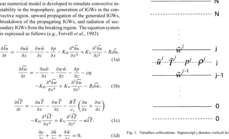
2.1 Basic equation system

A non-hydrostatic compressible two-dimensional nonlear numerical model is developed to simulate convective in-stability in the troposphere, generation of IGWs in the con-vective region, upward propagation of the generated IGWs, breakdown of the propagating IGWs, and radiation of sec-ondary IGWs from the breaking region. The equation system is expressed as follows (e.g., Forvellet al., 1992):

∂δu

whereu denotes horizontal wind,wvertical wind, T tem-perature,ρdensity,ppressure,ggravitational acceleration, Rgas constant for dry air,cvspecific heat of dry air at con-stant volume, KHhorizontal eddy diffusion coefficient,KV vertical eddy diffusion coefficient,RfRayleigh friction co-efficient, andαNewtonian cooling coefficient.

The product of the dynamical variables [u, w,T] andρ denoted by the tilde, for example,

˜

u(x,z,t)≡u(x,z,t)·ρ(x,z,t). (2)

Furthermore the deviation of the each variable from an initial basic state, which is independent of time, is denoted byδas follows: where the subscript B denotes the initial basic state.

2.2 Spectral and finite difference presentation of vari-able

The physical variables are expanded in the horizontal di-rection by the complex Fourier series as follows,

wherekdenotes horizontal wavenumber,KMthe maximum horizontal wavenumber, and the superscript ∗denotes the complex conjugate. In the vertical direction, a finite dif-ference method is used, and the variables are located on the

(3)

K. GOYA AND S. MIYAHARA: NON-HYDROSTATIC MODEL SIMULATION OF INTERNAL GRAVITY WAVES 487

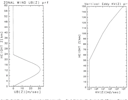
Fig. 2. Vertical profile of initial background horizontal windUB(z)(m s−1).

Fig. 3. Vertical profile of initial background temperatureTB(z)(K).

Fig. 4. Vertical profile of vertical eddy diffusion coefficientKV(z)(m2s−1).

(4)

(5)

(6)

Fig. 7. As in Fig. 6(c), except for the plots below 30 km height.

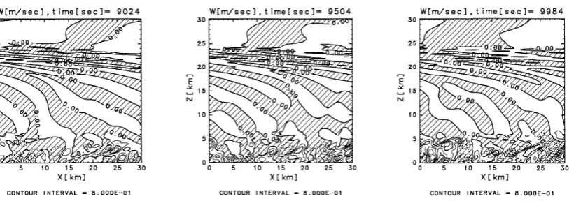
Fig. 8. As in Fig. 7, except for the time steps of 9,024 s, 9,504 s, and 9,984 s.

coefficientα(z)is assumed to be the same value withRf(z). They are given to prevent the spurious reflection from the top boundary. An uniform horizontal eddy diffusion coefficient

KHof the value of 8.0×107m4sec−1is used to prevent a spurious energy accumulation at the truncated wavenumber. The correct vertical diffusion scheme, for instance in (1a), is

∂ ∂z(ρKV∂

u

∂z). However, the simplified form shown in (1a) is used for simplicity in the present model. The difference of these two scheme is negligibly small for the parameter range in the present numerical simulation. Effects of eddy diffusion below 100 km in the numerical results are negligibly small.

3. Results and Discussions

3.1 Convection and IGWs propagation

Figures 6(a), (b) and (c) show the cross section of the total potential temperature, the horizontal wind fluctuation from the zonal mean, and the vertical wind in the troposphere, respectively, at the time steps of 4,800 s, 5,600 s, and 6,400 s. It is found that a disturbance having overturning potential temperature structure grows with time and moves eastward with the velocity which is almost equal to the background horizontal wind velocity at the height where the center of the disturbance is located. Compared with Figs. 6(b) and (c), it is found that the potential temperature disturbance corresponds to the strongest region of the horizontal and the vertical wind fluctuations. Other than the strongest disturbance, there are

(7)

Fig. 9. Space-time spectrum of the vertical windw(m s−1) at 12 km height for the time span from 8,000 s to 10,048 s. Positive horizontal wavenumber denotes eastward moving and negative denotes westward moving components.

Fig. 10. Vertical profile of square of horizontal wavenumberk2_associated

with waves ofm2₌_{0 for phase velocity}_c₌_{5 m s}−1_{(solid), 10 m s}−1

(dashed), 2.5 m s−1(dotted).

20 km height. These parameters of the wave approximately satisfy the following dispersion relation of IGWs assuming the mean temperatureT =250 K,

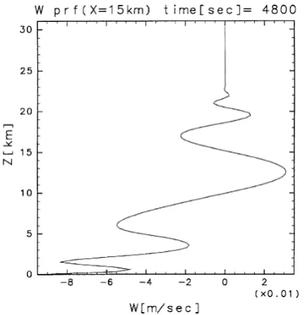
Fig. 11. Vertical profile of vertical wind (m s−1_{) at 4,800 s.}

ˆ

ω2 ₌ N 2_k2

k2+_m2+ 1 4H2

, ωˆ ≡ω−U k=(c− ¯U)k, (8)

where ωˆ denotes the intrinsic frequency, ω frequency, k horizontal wave number, m vertical wave number, Burant-Vais¨ all¨ a frequency, and the scale height is de¨ fined byH ≡RT/g. Thus the wave generated by the convection is identified as an IGW.

(8)

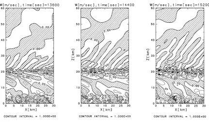
Fig. 12. Contour plots of vertical windw(m s−1) below 60 km height at the time steps of 13,600 s, 14,400 s, and 15,200 s. Negative values are shaded.

and higher frequency spectrum as shown in Fig. 9 than the IGW shown in Fig. 7. The phase velocities of the waves are about 10 m s−1_{, which are equal to the velocity of the} back-ground horizontal wind at the top boundary of the convective layer of 3–4 km height. It seems that the background hori-zontal wind in which the convection is embedded determines the phase velocity of them.

Substitutingu¯(z),N2₍_z₎_and_T ₌_{250 K into (8), vertical} profiles of square of horizontal wavenumberk2 _associated with the waves ofm2 ₌_{0 for}_c₌ _{5 m s}−1_,_c₌ _{10 m s}−1 andc =2.5 m s−1 are shown in Fig. 10. The left side of lines means that the waves become internal and the right side means that the waves cannot propagate vertically. It is found that the values ofk2 forc = 10 m s−1 at 9.6 km height indicates that the smallest wavelength is about 10 km with which the wave can propagate vertically. Thisfigure shows that the wave with the horizontal wavelength of the order of 10 km is chosen and shorter than that is filtered out by the background westerly. As the convection becomes more active with time, the level of the strongest disturbance in the convective layer is getting higher. The velocity of the background wind is larger with height in the convective layer, so that the horizontal phase velocity of the radiated dominant IGWs is getting faster. According to Fig. 10, it is found that the smallest wavelength of which the wave is internal becomes larger when the phase velocity gets faster. Larsenet al.(1982) observed stratospheric wave motions above tropospheric convections, and found a high frequency wave with a period of 6 min and the vertical wavelength of 7 km. The dominant waves in the present model simulation are consistent with these high frequency IGWs observed in the real atmosphere in spite of the difference of the convection mechanism.

3.2 IGWs-critical layer interaction and secondary wave radiation by critical layer instability

Figure 11 shows the vertical profile of vertical wind at x=15 km at the time of 4,800 s. Figures 7 and 11 show that the wave amplitude decreases and the vertical wavelength be-comes short and the phase line approaches horizontal above 20 km. As mentioned above, this behavior is due to the criti-cal layer interaction found by Booker and Bretherton (1967). As the time goes on, the critical layer structure becomes more complicated in the range from 18 km to 24 km height. Figure 12 shows the cross section of vertical wind below 60 km height at the time steps of 13,600 s, 14,400 s, and 15,200 s. At these time steps, it is found that the convection becomes more active, and the maximum vertical wind in the lower tropospheric convection exceeds 4 m s−1and the am-plitude of the IGW generated by the convection also reaches above 2 m s−1 _{above 16 km height. The wave pattern} be-comes random around the critical layer. It is found that the new eastward tilted wave pattern is propagating upward (the phase is moving downward and eastward) above the critical layer. These distributions show that the critical layer insta-bility of the incident IGWs and the secondary wave radiation by the instability.

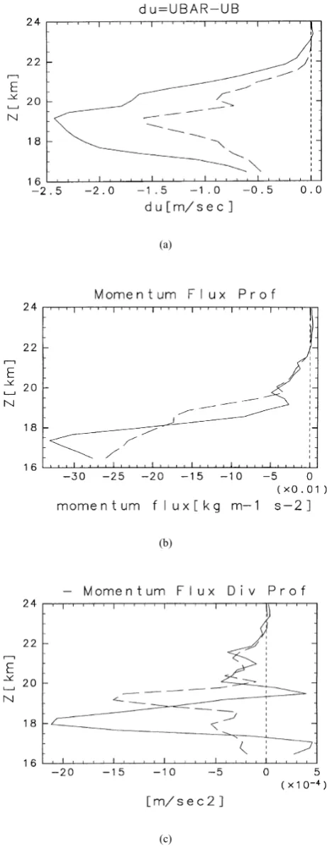
Figure 13(a) shows the deviation of the zonal mean wind from the initial basic state. There is a deceleration region below 23 km height and the strongest deceleration occurs at 19 km height. The relationship between the zonal mean wind U(z,t)and the momentumflux is given as follows, whereudenotes the deviation from the zonal mean wind,

w_{the vertical wind and overbar denotes the zonal mean.}

(9)

(a)

(b)

(c)

Fig. 13. Vertical profiles of (a) deviation of horizontal wind from the initial background horizontal windUB(z), (b) momentumflux, and (c) inverse

sign of vertical divergence of the momentumflux. Dotted, dashed, and solid lines show the values at 5,600 s, 13,600 s, and 15,200 s, respectively.

flux. It is found that the momentumflux decreases abruptly from 18 km to 22 km height. Figure 13(c) shows the mo-mentumflux divergence of RHS of (9). The peak value is

Fig. 14. Contour plots of potential temperature (K) at the time steps of 13,600 s, 14,400 s, and 15,200 s.

(10)

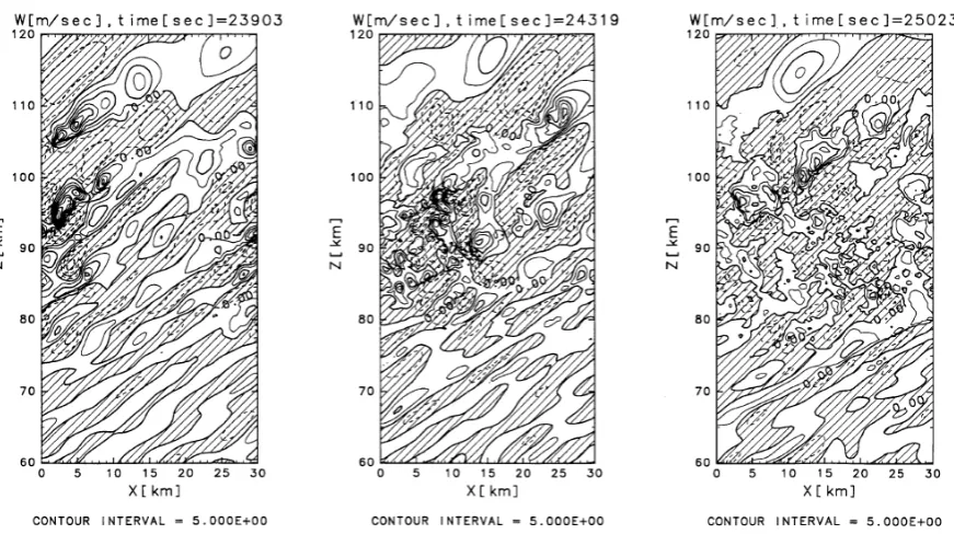
Fig. 15. Contour plots of vertical windw(m s−1_{) at the time steps of 23,903 s, 24,319 s, and 25,023 s.}

Fig. 16. As in Fig. 15, except for the potential temperature.

atmosphere. Thus intermittent structure may reduce the net momentumflux in the real atmosphere.

Figure 14 shows the contour plots of the potential temper-ature from 18 km to 22.5 km height. Local overturning of the isentropic lines is seen and it shows the convective instability of the incident waves around the critical layer. This insta-bility generates the random pattern of the critical layer and radiates secondary waves. The space-time spectral analysis

(11)

Fig. 17. Vertical profiles of momentumflux time-averaged over 7.5 min interval associated with the wave K1 (solid line), K5 (dashed line) and K6 (dotted line). Time average is done over 18,016 s–18,464 s, 21,984 s–22,432 s, and 25,536 s–25,984 s.

the vertical wavelength of k1 is also deduced to be 13 km. Doppler-shift is negligible above 24 km height because there are no zonal mean winds. These parameters of the waves satisfy the dispersion relation (8), so that secondary radiated waves are also identified as IGWs. As the case of IGWs generation by the convection, the zonal mean wind velocity of the secondary wave source region determines the phase velocity of the secondary wave. However the wave k1 is not the case and the phase velocity is much faster than the zonal wind velocity. It is not cleared the generation mechanism of the IGW with fast phase velocity. In the unstabilized critical layer, the nonlinear interaction becomes strong, then it might be possible to generate the wave k1 by the nonlinear inter-actions. But the present work is focusing on the propagation of IGWs throughout the middle atmosphere, so that we do not deeply investigate the generation mechanism. It will be done in a separate paper.

3.3 IGWs breakdown in the upper middle atmosphere Figure 15 shows that the contour plots of vertical wind from 60 km to 120 km height at the time steps of 23,903 s, 24,319 s, and 25,023 s after about 3 hours shown in Fig. 12. Figure 16 shows that the contour plots of potential temper-ature at the same time steps. It is found that the secondary IGWs radiated by the critical layer instability in the lower stratosphere break in the upper mesosphere and the breaking region spread downward with the time goes on, and turbulent layer is generated. It is also found that the IGWs propagates vertically in the form of wavepackets and break by local con-vective in stability due to the exponential growth of the wave amplitude with height. In the previous section, it is shown that the main IGWs generated by the critical layer instability are the eastward moving waves k5, k6 and k1. The vertical space spectral analysis, which is conducted using the data from 40 km to 78 km, the waves with zonal wavenumbers k =5,k=6 andk=1 have representative vertical

wave-lengthλV6 km, 6 km, and 13 km, respectively. The group velocitycgzof an IGW is given by the following equation;

cgz= −N m|k|

(k2+_m2+ 1 4H2)3/2

. (10)

(12)

(a)

(b)

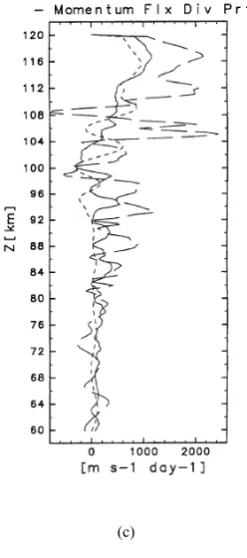
Fig. 18. Vertical profiles of (a) deviation of horizontal wind from the initial background horizontal windUB(z), (b) momentumflux, and (c) inverse

sign of vertical divergence of the momentumflux. Dotted, dashed, and solid lines show the values at 21,120 s, 23,520 s, and time-averaged over 23,552 s–25,984 s, respectively.

decreases with height and the westerly acceleration occurs in the upper mesosphere and lower thermosphere, except for some irregularities. The instantaneous acceleration of the

(c)

Fig. 18. (continued).

zonal mean wind due to the breakdown is the order of 103 m s−1_day−1_{at 93 km as indicated by the dashed line, but the} height and time-averaged acceleration is of the order of 102 m s−1_day−1_{, which is the same order of theoretical} estima-tions and observational reports about the momentumflux in this region (e.g., Lindzen, 1981; Fritts and Vincent, 1987). It is noted that our simulation assumed the continuous con-vective instability in both the time and space, so that the momentumflux might be much larger than that induced by convectively generated IGWs in the real atmosphere, and the deceleration in the real atmosphere cannot be attributed to the gravity waves generated by the present mechanism.

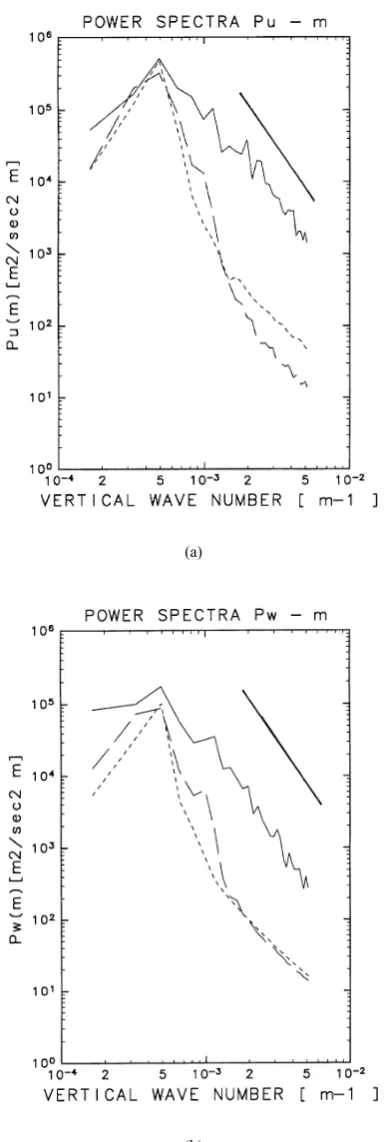
Figures 19 (a) and (b) show the power spectra of the hor-izontal and vertical wind in the wavenumber space m be-tween 80 km and 118 km heights, respectively. It is found that the power spectra show approximatem−3 _dependence at higher wavenumber region after the waves are breakdown (t = 24,320 s). Such dependence has been reported by VanZandt (1982) for the horizontal wind spectra, and it is also reported for the vertical wind spectra by Fritts and Hoppe (1995). It is predicted that the dependencem−3_{is due to the} wave saturation and breakdown (Dewan and Good, 1986), and it is shown that such the universal power law is also realized after the wave breaking in the present model.

4. Conclusions and Remarks

(13)

(a)

(b)

Fig. 19. Power spectra versus vertical wavenumbermat between 80 km and 118 km, (a) for the horizontal velocity deviation from the zonal mean, and (b) for the vertical velocity. Dotted, dashed, and solid lines show the values at 19,840 s, 21,440 s, and 24,320 s, respectively. Thick solid line has a slope ofm−3.

IGWs are radiated from the critical layer through the critical layer instability, and these waves breakdown and accelerate the zonal mean wind in the upper middle atmosphere due to

local convective instability because of the exponential growth of the amplitude with height.

In the present work, the followings are demonstrated: It is realized that the first IGWs have small wavelength of about 10 km with the aspect ratio k/m of about 1 and short period of about 10 min. It is found that this fact results from the process that the waves with the smallest horizontal wavelength which can propagate vertically in the prescribed westerly is selected. The background zonal mean wind in the convective layer determines the phase velocity of the dominant IGWs in both cases of the convective wave gen-eration and the critical layer wave gengen-eration. However, in the secondary IGWs radiated from the unstabilized critical layer, the wave with the phase velocity much faster than the background zonal mean wind velocity is also seen.

The deceleration due to the IGWs-critical layer interaction is instantaneously marked by−180 m s−1_day−1_{. This value} is much larger than the value due to gravity wave parame-terization introduced to some general circulation models to realize the weak zonal mean winds in the lower stratosphere (e.g., McFarlane, 1987). However the present results are not surprising, because the present model always generates grav-ity waves keeping the convectively unstable situation. In the realistic situation, gravity waves may be more sparse both in the space and the time.

The IGWs generated by the critical layer instability be-gin to break in the upper mesosphere and the breakdown region spreads down to the lower mesosphere atmosphere with time. The first propagating wave is λH 30 km (K1), and the next propagating waves areλH6 km and 5 km (K5 and K6, respectively). K1 breaks in the upper level, and K5 and K6 breaks in the lower level. The breakdown strongly depends on the exponential growth of the amplitude with height. The difference of the breaking level depends on the amplitudes of the wave and the vertical wavelength. The waves K5 and K6 have larger amplitude and shorter vertical wavelength than the wave K1, so that the breaking level is lower than that of K1. The magnitude of acceleration in the IGWs breaking region is about 100 m s−1_day−1_{, which has} same order magnitude with the momentum deposition by the-oretical estimations and observational reports (e.g., Lindzen, 1981; Fritts and Vincent, 1987). It is noted that our simula-tion assumed the continuous convective instability in both the time and space, so that the momentumflux might be much larger than that induced by convectively generated IGWs in the real atmosphere, and not all the deceleration in the real atmosphere can be attributed to the gravity waves generated by the present mechanism. It has been considered that IGWs are important source of momentum in the upper middle at-mosphere and they propagate directly from the troposphere without breakdown on the way. However the present result suggests the importance of the secondary generated waves due to the breakdown of the primary waves on the way.

The power spectra of the wind fluctuation shows m−3 dependence on the vertical wavelength in the upper meso-spheric breaking region. The universal power law which is due to the wave saturation and breakdown is observed in the real atmosphere and theoretically predicted (VanZandt, 1982; Dewan and Good, 1986).

(14)

are now conducted, and the results will be shown in a separate paper.

Acknowledgments. The authors wish to express their thanks to Drs. T. Hirooka, K. Sato, K. Nakajima, Y. Miyoshi, and T. Iwayama for their valuable comments and suggestions. The GFD-DENNOU Library was used for drawing thefigures.

References

Alexander, M. J., J. R. Holton, and D. R. Durran, The gravity wave response above deep convection in a squall line simulation,J. Atmos. Sci.,52, 2212–2226, 1995.

Asai, T., Stability of a plane parallelflow with variable vertical shear and unstable stratification,J. Meteor. Soc. Japan.,48, 129–139, 1970. Booker, J. R. and F. P. Bretherton, The critical layer for internal gravity

waves in a shearflow,J. Fluid. Mech.,27, 513–539, 1967.

Bretherton, F. P., The propagation of groups of internal gravity waves in a shearflow,Q. J. R. Meteorol. Soc.,92, 466–480, 1966.

Dewan, E. M. and R. E. Good, Saturation and the“universal”spectrum for vertical profiles of horizontal scalar winds in the atmosphere,J. Geophys. Res.,91, 2742–2748, 1986.

Forvell, R. G., D. Durran, and J. R. Holton, Numerical simulations of con-vectively generated stratospheric gravity waves,J. Atmos. Sci.,49, 1427–

1442, 1992.

Fritts, D. C., The excitation of radiating waves and Kelvin-Helmholtz insta-bilities by the gravity wave-critical level interaction,J. Atmos. Sci.,36, 12–23, 1979.

Fritts, D. C., The transient critical-level interaction in a Boussinesqfluid,J. Atmos. Sci.,87, 7997–8016, 1982.

Fritts, D. C. and U. P. Hoppe, High-resolution measurements of vertical velocity with the European incoherent scatter VHF radar 2: Spectral observations and model comparisons, J. Geophys. Res.,100, 16827–

16838, 1995.

Fritts, D. C. and G. D. Nastrom, Sources of mesoscale variability of gravity waves II: Frontal, convective, and jet stream excitation,J. Atmos. Sci.,

49, 111–127, 1992.

Fritts, D. C. and R. A. Vincent, Mesospheric momentumflux studies at

Adelaide, Australia: observations and a gravity wave-tidal interaction model,J. Atmos. Sci.,44, 605–619, 1987.

Fritts, D. C., J. R. Isler, andØ. Andreassen, Gravity wave breaking in two and three dimensions 2: Three-dimensional evolution and instability structure,J. Geophys. Res.,99, 8109–8123, 1994.

Geller, M. A., H. Tanaka, and D. C. Fritts, Production of turbulence in the vicinity of critical levels for internal gravity waves,J. Atmos. Sci.,32, 2125–2135, 1975.

Hodges, R. R., Jr., Generation of turbulence in the upper atmosphere by internal gravity waves,J. Geophys. Res.,72, 3455–3458, 1967. Larsen, M. F., W. E. Swartz, and R. F. Woodman, Gravity-wave generation

by thunderstorms observed with a vertically-pointing 430 MHz radar,

Geophys. Res. Lett.,9, 571–574, 1982.

Lindzen, R. S., Turbulence and stress owing to gravity wave and tidal break-down,J. Geophys. Res.,86, 9707–9714, 1981.

Matsuno, T., A quasi one-dimensional model of the middle atmosphere circulation interacting with internal gravity waves,J. Meteor. Soc. Japan.,

60, 215–226, 1982.

McFarlane, N. A., The effect of orographically excited gravity wave drag on the general circulation of the lower stratosphere and troposphere,J. Atmos. Sci.,44, 1775–1800, 1987.

Palmer, T. N., G. J. Shutts, and R. Swinbank, Alleviation of a systematic westerly bias in general circulation and numerical weather prediction models through an orographic gravity wave drag parameterization,Q. J. R. Meteorol. Soc.,112, 10001–10039, 1986.

Prusa, J. M., P. K. Smolarkiewicz, and R. R. Garcia, Propagation and break-ing at high altitudes of gravity waves excited by tropospheric forcbreak-ing,J. Atmos. Sci.,53, 2186–2216, 1996.

Sato, K., Small-scale wind disturbances observed by the MU Radar during the passage of typhoon Kelly,J. Atmos. Sci.,50, 518–537, 1993. Sato, K., Observational studies of gravity waves associated with convection,

Gravity Wave Processes, inNATO ASI Series, edited by K. Hamilton, pp. 63–68, Springer, 1997.

VanZandt, T. E., A universal spectrum of buoyancy waves in the atmosphere,

Geophys. Res. Lett.,9, 575–578, 1982.