R E S E A R C H
Open Access
2-D DOA tracking using variational sparse
Bayesian learning embedded with Kalman
filter
Qinghua Huang
*, Jingbiao Huang, Kai Liu and Yong Fang
Abstract
In this paper, we consider the 2-D direction-of-arrival (DOA) tracking problem. The signals are captured by a uniform spherical array and therefore can be analyzed in the spherical harmonics domain. Exploiting the sparsity of source DOAs in the whole angular region, we propose a novel DOA tracking method to estimate the source locations and trace their trajectories by using the variational sparse Bayesian learning (VSBL) embedded with Kalman filter (KF). First, a transition probabilities (TP) model is used to build the state transition process, which assumes that each source moves to its adjacent grids with equal probability. Second, the states are estimated by KF in the variational E-step of the VSBL and the variances of the state noise and measurement noise are learned in the variational M-step of the VSBL. Finally, the proposed method is extended to deal with the off-grid tracking problem. Simulations show that the proposed method has higher accuracy than VSBL and KF methods.
Keywords:2-D direction-of-arrival (DOA) tracking, Spherical array, Transition probabilities (TP) model, Variational sparse Bayesian learning (VSBL), Kalman filter (KF)
1 Introduction
Direction-of-arrival (DOA) estimation is an active re-search field of array signal processing and has been used in various applications, such as radar, channel modeling, tracking, and surveillance [1–3]. Among the estimation al-gorithms, multiple signal classification (MUSIC) and esti-mation of signal parameters via rotational invariance techniques (ESPRIT) are the most representative methods, which employ the signal and noise subspaces. Compared with the conventional beamforming algorithms, these methods enhance the estimation precision. However, the number of impinging signals must be the prior knowledge and the computational complexity of decomposing the covariance matrix increases when the number of array elements rises. Recently, sparse reconstruction methods have attracted substantial attention because the signals impinging on an array are intrinsically sparse in the spatial domain [4, 5]. In these methods, the whole angular domain is divided into some predefined grids and a meas-urement matrix is constructed by sampling these grids.
Based on the singular value decomposition (SVD), an ap-proach named as l1-SVD was proposed to reduce the computational complexity and enforce sparsity using l1 -norm [6]. Compared with the l1-SVD method, sparse Bayesian learning (SBL) can model the sparse signals more flexibly and give more accurate recovery results [7–9]. When SBL was used to estimate DOA, the sparse prior for the interested signals is Gaussian [10] or Laplacian distribution [11]. The SBL method can achieve good esti-mation results for static DOA estiesti-mation.
In the case of tracking moving targets, most methods as-sume that each source angle is constant during a time interval. However, it may differ from one interval to an-other because of the moving sources [12]. There are some different approaches to track the DOAs of moving sources, such as classical subspace optimization approach, sparsity recovery theory, and adaptive filter method. The subspace optimization approaches only optimize the signal or noise subspace without using the eigenvalue decomposition (EVD) so that they can reduce the computational complex-ity and storage requirements. Yang presented a new ap-proach to track the signal subspace using an unconstrained minimization method [13]. The subspace method, which * Correspondence:[email protected]
Key Laboratory of Specialty Fiber Optics and Optical Access Networks, Shanghai University, Shanghai 200072, People’s Republic of China
can be used to dynamic DOAs, was extended in L-shaped array [14] and two parallel linear arrays [15], respectively. The performance of the subspace method relies on the number of snapshots. This kind of method is inapplicable for the moving targets when the number of snapshots in each time interval is relatively small.
Vaswani et al. reviewed many algorithms on the analysis of dynamic sparse signal recovery. If the support change is highly correlated and the correlation model is known, we can get an accurate support estimation by using the previ-ous estimation information [16–18]. In [19, 20], these methods combined the slow signal value change and slow support change to enhance the precision. Most of these methods are the deformation of basis pursuit denoising. A sequential Bayesian algorithm was introduced to estimate the moving DOAs in the time-varying circumstance [21]. It assumed that the sources move at a constant velocity and used this hypothesis to construct the signal-moving model. The locally competitive algorithm (LCA) was pro-posed to construct a dynamic system and track DOAs [22]. This method mainly introduced a thresholding func-tion to enforce sparsity. A model was proposed to describe a time-varying array response in the frequency domain for each source [23]. The key of this paper is that it utilizes a hidden Markov model to describe the moving signal and uses the posterior inference to estimate the signal posi-tions. It traps into the local optimum when the signals alias at high frequency.
The Kalman filter (KF) method is the most repre-sentative method for tracking sources in the adaptive filter theory, which means the value of the predicted state should equal to the value of the actual state by minimizing the Bayesian mean square error of the state vector. However, the variance of the noise and state can be seen as prior in the KF method. In [24], the time difference of arrival (TDOA) information was calculated by a pair of microphones and a dis-tributed unscented KF method was used to track speakers in a nonlinear measurement model. The method combining KF with compression sensing was also used for dynamic DOA estimation [25, 26]. The state transition function was built under the assump-tion that the bearing change rate had been known [25]. This assumption is hard to be satisfied in real applications. A Bayesian compressive sensing Kalman filter (BCSKF) method [26] was proposed to track dy-namic moving sources. This method used the con-stant DOA changes in the KF prediction, which meant that the source moved to the designated direc-tion with a fixed step. The particle filter was utilized to track the trajectory of target. It adopted a series of particles to represent the posterior distribution of sig-nal stochastic process. For example, an algorithm combining compressive sense and particle filter was
introduced in [27]. However, it only used the com-pressive sense to estimate the original position and utilized particle filter to track the trajectory.
In this paper, a spherical array is used to track the moving sources in 3-D space because the array is 3D symmetric structure and can capture high-order sound field information [28–30]. Besides, comparing with linear array, spherical array can capture the two-dimension information of signal rather than single-angle information. In addition, due to the special con-struction of spherical array, the receiving signal can be unfolded in special harmonic domain, which can separate the signal position coordinates and sensor position coordinates conveniently.
A new method is proposed based on the spherical array to track the 2-D dynamic DOAs. It combines the variational Bayesian inference and KF to improve the tracking performance. First, a transition probabil-ities (TP) model is built to describe the state transi-tion process of a signal. In this model, the source moves to an uncertain situation with an equal prob-ability rather than a determining expected DOA change in [26]. In addition, TP model is convenient to build with a tracking framework and adopts sparse methods to estimate signal position. Based on this model, an alternating iterative method is developed to track DOAs. In the first step, we use the KF method to estimate the signal values. In the second step, we use variational sparse Bayesian learning (VSBL) to learn the variances of the measurement noise and state noise, which are useful to update the signal state in the KF method. This is an interdependent process.
There are three differences between the proposed ap-proach and the method appeared in paper [26]. On the one hand, the proposed method constructs a real-valued steering matrix in signal model rather than split-ting the complex value into several real-valued ones, which can reduce a half of the computational quantity approximately. On the other hand, the KF estimation values is used instead of the Bayesian estimation values. The main contribution of paper [26] is putting the esti-mation parameters of KF to optimize the low bound of relate vector machine. However, the KF estimation will be embedded in VSBL to improve the precision further in this paper. Finally, we introduce the off-grid model to overcome the mismatch problems.
The rest of the paper is organized as follows. The real-valued array signal model is given in Section 2. The variational Bayesian inference is briefly reviewed, and the proposed tracking method is introduced in Sections 3 and 4. Numerical examples and simulation results are given in Section 5. Section 6 concludes the paper.
(a,b,A,B,⋯), scalar variable arg(⋅), phase operator
(⋅)H, conjugate transpose operator ‖⋅‖F, Frobenius norm
diag(⋅), diagonal matrix 〈⋅〉, expectation operator
blkdiag(⋅), block diagonal matrix A(n, :), thenth row of matrixA
Re(⋅), the real parts of a complex value A(:,n), thenth column of matrixA
exp(⋅), the exponent signal Im(⋅), the imaginary parts of a complex value
k, the wavenumber D, the number of signals
(ϑl,φl), the elevation and azimuth
azimuth of thedth signal at thetth time interval
L, the number of sensors t, time interval
B, snapshots R, the radius of sphere array
G1,G2, the azimuth and elevation range i, the imaginary unitpffiffiffiffiffiffi−1 sparse amplify signal and the real-valued amplify signal
ð^V;V;VÞ, the space domain, the spherical and the real-valued noise
hn, spherical Hankel function
of ordern
Ym
nðÞ, the spherical harmonic
of ordernand degreem
In, ann × nidentity matrix jn, then-order spherical Bessel
function
Jn, the exchange matrix with ones on its antidiagonal and zeros elsewhere
(⋅)', the derivation operators
Γ(⋅), a Gamma function 0n, a column vector containing nzeros
(A\b), take the variablesAexcept variableb
2 Real-valued array signal model
AssumingDdynamic narrowband far-field signals with the
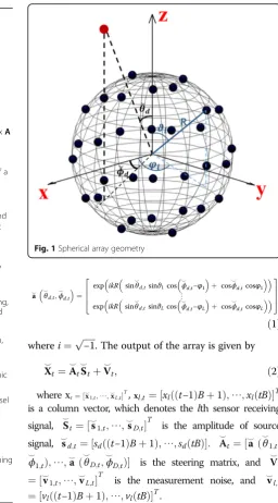
wavenumberkimpinge on a spherical array fromΦ^d;t ¼ ð able to process the received data and estimate DOA in each time interval. We usetto represent the range [(t−1)B+ 1, ⋯,tB] for simplicity. The signal angular change is slow so that it can be considered as fixed in the time intervalt. The spherical array is made of L identical isotropic elements with radiusRin Fig.1. The position of thelth sensor can be described as Rl=R[cosφlsinϑl, sinφlsinϑl, cosϑl]T. The
steering vector of the array is defined as
a is a column vector, which denotes the lth sensor receiving
signal, ^St¼ ½s
is the amplitude of source
signal, ^sd;t¼ ½sdððt−1ÞBþ1Þ;⋯;sdðtBÞ: A
In order to construct a sparse signal model, we divide the azimuth and elevation range into G1> >D and
G2> >Dgrids, respectively. That is to say, the whole 2-D angular space is divided intoG=G1G2grids noted as Φ= {Φ1,⋯,ΦG}, where Φg ¼ ðθg1;ϕg2Þ, g1= 1, ⋯, G1, g2= 1, ⋯, G2. The output of the sensors at the time intervaltcan be reformulated as
X dictionary matrix containing the interested angles Φ^d;t,
d= 1, ⋯, D, and St ¼ ½s1;t;⋯;sG;tT is a sparse matrix with only D nonzero rows corresponding to the positions of the sources. ^alðΦgÞdenotes thelth element
of the dictionary vector ^a ðΦgÞ , and it can be represented using spherical harmonics [31] as
a ^
l Φg ¼ XN
n¼0
Xn
m¼−n
bnð ÞkR Ymn Φg
Ymnð ÞΩl ; ð4Þ
where Ωl= (ϑl,φl), N is the maximum spherical
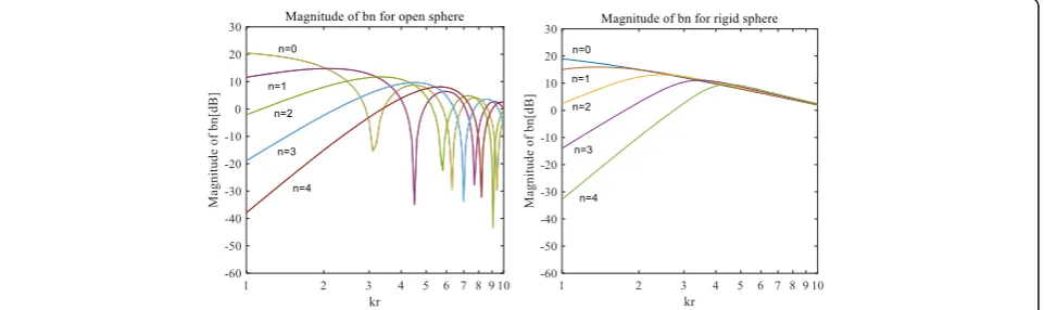
harmonics order, bn(kR) is the far-field mode strength, which depends on the array properties. The simplest spherical array configuration is the open sphere composed of sensors suspended in free space. It is assumed that the other accessories, such as cables and mounting brackets, have no effect for sensors capturing. However, this configuration might make the open sphere suffer from poor robustness at some certain frequency points. Another common configuration is the rigid sphere. In this configuration, sensors are mosaicked on a rigid spherical baffle, which means the sound waves will be scattered by the sphere. So, the mode strength of these two configurations is different. The magnitude of
bn(kR)for different sphere is shown in Fig.2. The specific form can be expressed as
bnðkRÞ ¼
f
4πinjnðkRÞ open sphere
4πin j nðkRÞ−
j′nðkRÞ
h′nðkRÞ
hnðkRÞ
!
rigid sphere; ð5Þ
Ym
nðθ;ϕÞdefined as:
Ymnðθ;ϕÞ ¼
ffiffiffiffiffiffiffiffiffiffiffiffiffiffiffiffiffiffiffiffiffiffiffiffiffiffiffiffiffiffiffiffi 2nþ1
4π
n−m ð Þ!
nþm
ð Þ!
s
PmnðcosθÞeimϕ; ð6Þ
where 0≤n≤N, −n≤m≤n, and Pm
nðcosθÞ are the associated Legendre polynomials [32].
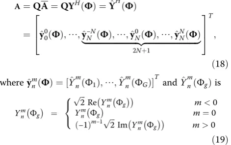
According to (4), the dictionary matrix A^ can be written as
^
A¼Yð ÞΩ Bð Þk YHð ÞΦ ; ð7Þ
where Y(Ω) is an L×J spherical harmonic matrix whoselth row is given as:
yð Þ ¼Ωl Y|fflfflffl{zfflfflffl}00ð ÞΩl n¼0
;Y|fflfflfflfflfflfflfflfflfflfflfflfflfflfflfflfflfflfflfflfflffl{zfflfflfflfflfflfflfflfflfflfflfflfflfflfflfflfflfflfflfflfflffl}−11ð ÞΩl ;Y10ð ÞΩl ;Y11ð ÞΩl n¼1
;⋯;|fflfflfflfflfflfflfflfflfflfflfflfflfflfflfflfflffl{zfflfflfflfflfflfflfflfflfflfflfflfflfflfflfflfflffl}Y−NNð ÞΩl ;⋯;YNNð ÞΩl n¼N
;
ð8Þ
where J= (N+ 1)2, Y(Φ) is a G×J spherical harmonic matrix defined similarly to Y(Ω), and B(k) is a J×J far-field mode strength matrix:
Bð Þ ¼k diag
b0ð ÞkR
|fflfflffl{zfflfflffl} n¼0
;b|fflfflfflfflfflfflfflfflfflfflfflfflfflfflfflfflfflffl{zfflfflfflfflfflfflfflfflfflfflfflfflfflfflfflfflfflffl}1ð ÞkR ;b1ð ÞkR ;b1ð ÞkR
n¼1
;⋯;b|fflfflfflfflfflfflfflfflfflfflfflfflfflfflffl{zfflfflfflfflfflfflfflfflfflfflfflfflfflfflffl}Nð ÞkR ;⋯;bNð ÞkR n¼N
:
ð9Þ
From (7), the dictionary matrix consists of three terms. The first and the second terms are only correlated with the sensor positions and the wavenumber, respectively. Furthermore, considering Y(Ω)B(k) is anL×Jmatrix (L≥J) that has a left pseudo inverse, (3) can be rewritten as:
Xt ¼AStþVt; ð10Þ
where Xt ¼B−1ðkÞYþðΩÞX^
t, A¼YHðΦÞ, and Vt
¼B−1ðkÞYþðΩÞV^
t. Owing to the special property of spherical harmonic function, the complex-valued model can be transformed into a real-valued one to reduce the computational complexity.
Because of the characterization of ½YmnðΦÞ¼ ð−1Þm
Y−m
n ðΦÞ for each element in A, we can transform A into a matrix with column conjugation property [33] for each order by Q1:
Q1Xt ¼Q1AStþQ1Vt; ð11Þ we can find that each order has the column conjugation property, which means we can transform the complex-valued matrix into a real-valued one by linear combinations. So, the transform matrix is built as: unitary transform matrixQ2, (11) can be changed into
Q2Q1Xt ¼Q2Q1AStþQ2Q1Vt: ð17Þ
We useXt~ ¼AStþVt~ to stand for (17) for simplicity. The new signal and noise matrices after the unitary transformation can be described as Xt~ ¼QXt and Vt~
¼QVt , where Q=Q2Q1. The real-valued dictionary
matrix can be inferred as follows:
A¼QA¼QYHð Þ ¼Φ Y^Hð ÞΦ
Afterwards,Xt~ ,St, andVt~ can be partitioned into real and imaginary parts which are combined as Xt ¼ ½Reð
~
XtÞ; ImðXt~ Þ, St¼ ½ ReðStÞ; ImðStÞ, and Vt¼ ½Reð ~
VtÞ; ImðVt~ Þ. Therefore, the complex model (11) can be transformed into a real-valued one as:
Xt ¼AStþVt: ð20Þ
Now, the real-valued signal model (20) is obtained in the spherical harmonics domain.
3 Variational sparse Bayesian learning embedded with Kalman filter (VSBLKF) for 2-D DOA tracking When signal sources move in the whole angular space, it is necessary to model the evolution of St in
time. Most of existing tracking state models [19, 20, 34] reveal the velocity information of the target movement. However, a TP model [35] is adopted to describe the movement of sources in a more practical way in this paper. It assumes that each source can transfer to its adjacent grids or stay at the current grid with an equal probability. So, the grid set D= {1,⋯,G} distributes in a plane with G1
rows and G2 columns and is divided into three types, the corner area (D1, D3, D7, and D9), the
marginal area (D2, D4, D6, and D8), and the center
area (D5). The corresponding relation between the
three areas and the angular grids (Φg) is shown in
Fig. 3. St= 1(gl, :) denotes the vector at the glth grid
during the time interval t−1. The probability of the vector moving to the gcth position during the time interval t is fij as follows
fg
Therefore, the vector in the gcth position at the time intervaltcan be expressed as Stðgc;:Þ ¼PGg
l¼1fglgcSt¼1ð
gl;:Þ. Considering the state noise exists in the process of transition, the state transition model can be described as
St ¼FSt−1þEt; ð22Þ
whereEtis the state noise.
In tracking dynamic targets, the most popular method is KF technique. It is based on Gaussian assumption. In the standard KF method, the covariance matrix of the state noise and the variance of the measurement noise are assumed to be known. However, in real applications, it is difficult to know these parameters. Because of the advantage of VSBL, which can model the sparse signal well, we want to introduce VSBL into the KF method to estimate the covariance matrix of the state noise and the measurement noise variances. Nevertheless, based on the model we construct, it might be infeasible to calculate the posterior distribution. Because the dimensionality of the latent parameters is too high to calculate directly. Therefore, we attempt to turn to approximation schemes for help. The marginal probability of the observed data X is gotten by integrating over the remaining unobserved variables θ(including the latent variables S and some hyper-parameters) [36].
Pð Þ ¼X
Z
PðX;θÞdθ: ð23Þ
However, it is knotty to solve this integration. The variational approaches can be used to solve this problem by pulling in a distribution Q(θ) which allows the
marginal log likelihood to be decomposed into two terms
lnPð Þ ¼X L Qð Þ þKL Qð ‖PÞ; ð24Þ
L Qð Þ ¼
Z
Qð Þθ lnPðX;θÞ
Qð Þθ dθ; ð25Þ
whereKL(Q‖P) is the Kull-Leibler divergence between
Q(θ) and the posterior distribution P(θ|X) and it is Furthermore, because the left side of (24) is independent of Q(θ), maximizing L(Q) is tantamount to minimizing
KL(Q‖P). ThereforeQ(θ) represents an approximation to
the posterior distribution P(θ|X). The goal in a variational approach is to choose a suitable form for
Q(θ) which is adequately simple and flexible. Besides, it
should make the lower bound L(Q) to be readily evaluated and tight. In fact, some family of Q(θ)
distributions can be chosen and the best approximation within this family is found by maximizing the lower bound with respect to Q(θ). One approach is to assume
some tractable forms forQ(θ) and then to optimizeL(Q) about the parameters of the distribution [36, 37]. We adopt an alternative step and consider a factorized form over the component variables {θζ} inθas follows
Qð Þ ¼θ Y ζ
Qζð Þθζ : ð27Þ
This scheme is called a mean field theory [38]. Because of the true posterior distribution might not be calculated, an approximate distribution is introduced to estimate the distribution. In this paper, the mean field theory is adopted as the tool to solve above problem. In this method, we only limit the type range of probability distribution rather than the form of probability distribution, which can make the approximate distribution become more flexible and extensive. In the scenario considered, the signal is sparse in the whole space at each time interval, the potential position and noise variance can be seen as the unobserved variables, and the array receiving the signal can be seen as the observation variables. Therefore, the final model can be solved with the VSBL [39]. In the mean field theory of the posterior, the algorithm can optimize one parameter at a time while fixing all other parameters. The optimal distribution for each of the parameters can be expressed as:
where μ indicates one of the parameter and 〈lnp(X,θ)〉θ\μ is the expectation of the joint probability of the data and latent variables which take over all variables except μ.
pð Þ ¼Et ℳNG;2B 0;Σtjt;IG
Since the measurement noise satisfies Gaussian distribution, we can get
measurement signal can be expressed as
pðXtjSt;ΔtÞ ¼ℳNJ;2BðASt;Δt;I2BÞ
Equivalently, we introduce a conjugate prior over the inverse noise variance Δt given by Gamma
distribution:
The Eq. (31) will be the exponential form of quadric function about variable St, when the variableΔtis seen
as a constant. Therefore, the conjugate prior of St will
obey the Gaussian distribution [36]. So, the prior distribution ofStis
pðStjFSt−1;ΛtÞ ¼ℳNG;2BðFSt−1;Λt;IGÞ
The signal satisfies Gaussian distribution with zero mean. The variance of St is Λt ¼ diagðα−t1Þ, where hyperparameter αt= [α1, t,⋯,αG, t]. At the same time,
the conjugate prior ofαg,tsatisfies Gamma distribution
pαg;t¼Gamαg;tjag;t;bg;t¼bag;tg;tαg;tag;t−1e−bg;tαg;t=Γag;t; ð34Þ
where Γ(⋅) is a Gamma function [40]. The expectation of αg, t in (34) is 〈αg, t〉=ag, t/bg, t. Note
that the marginal distribution of St can be obtained
by integrating over αt. Note that if the prior
distribution and likelihood function conjugate each other, it will make the posterior distribution to have the same form with prior distribution [36].
Using the chain rule of probability [39], the posterior probabilistic distribution can be expressed as:
pðαt;St;ΔtjXtÞ∝pðXtjSt;ΔtÞpðStjαtÞpð Þpαt ð ÞΔt : ð35Þ
The variational framework introduces a factorial representation (27) approximating to the posterior distribution p(αt,St,Δt|Xt) by Q(αt,St,Δt) =Q(St)Q(αt) Q(Δt). We propose the VSBLKF algorithm using the
expectation maximization (EM) updates. In order to compute the E-step, it needs to know the posterior distribution of the unknown sparse state signal, which is Gaussian with mean Ut∣t and covariance Σt∣t.
These parameters can be computed by using KF pre-diction and updating equations as follows:
Predict steps:
Here, the initial value U0|0 can be assumed to be
known. In the M-step, we use VSBL to calculate the state variance and measurement variance of the current time. According to the Eq. (28)
Λg;t
¼ag;t=bg;t; ð45Þ
The posterior distribution of the noise inverse variance can be similarly calculated as
Qð Þ ¼Δt YJ
j¼1
Gam Δj;tjb Δ ð Þ j;t;cj;t
: ð46Þ
cð ÞjΔ;t ¼cð ÞjΔ;t þ0:5 ðXt−AStÞðXt−AStÞT
D E
; ð47Þ
bð ÞjΔ;t ¼bð ÞjΔ;t þ J; ð48Þ
Δj;t
¼bð ÞjΔ;t =cj;t; ð49Þ
where the hyperpriors ag;t;bg;t;bðΔÞj;t;cj;t are set as 10‐3. From (38), we can see that using these recursions cannot guarantee the prediction sparse. Running (38) up to a large enough t, the signal strength of this target will spill over to all entries of Ut∣t. So, we propose a state corrector method to
determine the true moving direction of next time and guarantee the prediction sparse. For each signal, there are different possible positions at next time. These possible positions correspond to nonzero values in Ut∣t noted as Utjtðp1;:Þ;⋯;UtjtðpPD
d¼1wd
;:Þ, where wd∈{4, 6, 9}. The value in the set correspond to different signal positions—corner area, marginal area, and central area successively. We find D
maximum values in Ut∣t corresponding to the
maximum of ‖[A(:,pκ)]TXt‖2, where κ¼1;⋯; PD
d¼1
wd; and consider these positions as true directions. At the same time, the rest of the rows in Ut∣t are
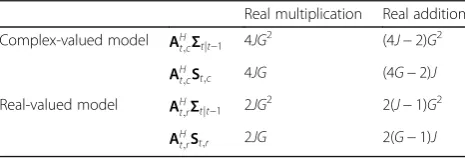
set to zeros. The steps of the proposed algorithm are summarized in the following. After that, we discuss the computational complexity of two models using VSBLKF to track DOA trajectory. The two models are the traditional complex-valued model and the proposed real-valued model, respectively. Different models lead to different measurement matrix dimen-sions, which may affect the parameter updates in VSBL. Table 1 shows the amount of computations using the two models. At, c, Xt, c, St, c and At, r, Xt,
r, and St, r represent the measurement matrices,
receiving data and sparse signals in the complex-valued model and real-complex-valued model. Real multiplica-tion and real addimultiplica-tion are used to evaluate the com-putational cost. Our proposed real model transforms the complex-valued measurement matrix into a real-valued one through a unitary transformation without changing the dimension. After the real-valued trans-form, the computation complexity for each iteration will reduce much when the steering matrix is used to calculate. Therefore, using the real-valued trans-form can improve the rate of the proposed algo-rithm. A unitary transformation needs 4J2T real multiplications and (4J−2)JT real additions, and it does not join the iteration of SBL. The computational load of the real-valued model is much lower than that of the complex-valued model, so the computation complexity can be reduced greatly.
4 Extension to off-grid problem
The assumption that the estimated signal directions lie on specified grids is unrealistic. To reduce the
Table 1Comparison of computational load in one iteration
Real multiplication Real addition
Complex-valued model AH
t;cΣtjt−1 4JG
2
(4J−2)G2
AH
t;cSt;c 4JG (4G−2)J
Real-valued model AHt;rΣtjt−1 2JG
2 2(J−1)G2
AH
errors which are caused by mismatch of the real lo-cations and partition lolo-cations, the denser grids can be applied when dividing the measurement matrix of signal. Nevertheless, each column of the measure-ment matrix needs to satisfy the cross-unrelated property for sparse recovery. The denser grids might lead to a higher complexity and make the dictionary become coherent that violates the necessary condi-tions for compressive sensing. Hence, to make the proposed algorithm more practical, the off-grid model is considered. As mentioned earlier, the direc-tional matrix Y^HðΦÞ in the VSBLKF algorithm is constructed on the uniform sampled angle grids Φ = {Φ1,⋯,ΦG} with Φg= (θg,ϕg), g= 1, ⋯, G. The tar-to Φg. In addition, we define the nearest grid of
tar-get signal angles as Φ^gd ¼ ð^θgd;ϕ^gdÞ. The true
steering vector aðΦ~dÞ can be approximated by its Taylor extension as [41].
a Φ~d ≈a Φ^gd
whereaðΦ^gdÞrepresents the original steering vector,b
ð^θgdÞ and cðϕ^gdÞare the partial derivative of θ diag(γ) can replace the original steering matrix A to estimate both signal coarse girds and their bias with elevation and azimuth, simultaneously. According to [41], the author solved this problem from the Bayes-ian perspective. In this section, we use the least squares estimation to calculate the biases of eleva-tion and azimuth, respectively. In the first step, we use VSBL to get the coarse estimation of true loca-tion. Next, using the expectation Ut∣t to minimize
the following equation as
where βξ stands for the kth iteration update of β and γξ represents the ξth iteration update of γ. When
updating difference biases, we keep another one fixed. It is tantamount to the least squares problem when we want to solve ation update ofβis:
βξ ¼ BΞξ
γξ ¼ CΞξ Stjt
þ
Xt− AþBdiag βξ
Uξ
tjt
: ð61Þ
The initial value of β and γ are set as 0G (a
col-umn vector containing G zeros). The number of source signals is known a priori. Each signal current coarse location can be approximated by VSBLKF and the biases between the reference and estimation are gauged using (59) and (60), respectively. The con-crete steps are summarized in Algorithm 2.
5 Results and discussion
In this section, we want to verify the robustness and performance of the proposed algorithm compared with the standard KF, SBL, and VSBL methods. We use a rigid spherical array, which has 32 sensors dis-tributed in a uniform way and radius R= 0.1 m. The maximum order of the spherical harmonics is N= 4. In our experiments, the ranges of elevation and azi-muth are defined from 0° to 180° and from 0° to 360°. We divide them into 31 and 62 grids with sta-tionary angular interval respectively. Therefore, there are 1922 grids which are the possible angles for source signals. Note that we only choose the range of azimuth from 0° to 180° in our simulations to re-duce the calculate complexity. In the moving process, assuming each source is likely to move to its adjacent grids or stay at current grid, which means a source can move to the different directions with 6° or be static with equal probability. The pro-posed method can track other trajectories as long as the trajectory can be described by the grids and obey the TP model. The trajectory used in this paper is randomly generated under the frame of TP model. In order to show a series of performance quantita-tively, such as on-grid, off-grid, and RMSE vs SNR, we used one trajectory to explain these results. One random realization of this movement model is con-sidered for T = 50 time interval. The number of Monte Carlo trials is 500. The hyperpriors ag;t;bg;t;
bðΔÞj;t ;cj;t are set as 10‐3.
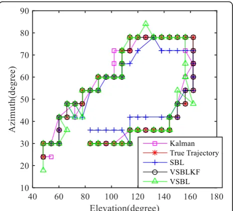
5.1 Example 1: the performance of the proposed method with an on-grid model
In the first simulation, we show the tracking per-formance of one signal at each time interval. The sig-nal to noise ratio (SNR) is set as 12 dB while the strength of the signal is 10. The moving trace ob-tained by the four methods are shown in Fig. 4. Figures 5 and 6 give the tracking performance at dif-ferent time intervals. The performance of SBL is poor, because the likelihood function of the measure-ments involved in SBL cannot match the true one.
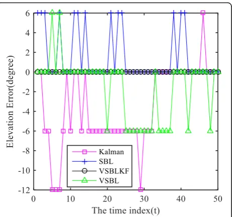
We can see that the VSBLKF method achieves the best tracking performance because it combines the advantages of KF with VSBL method. Figures 7 and 8 denote the signal angle errors (the differences be-tween the estimated angle and reference angle) vary-ing with time intervals. From these curves, the proposed method is better than the other approaches.
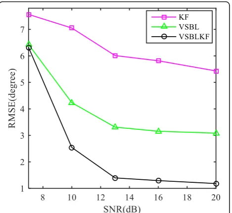
5.2 Example 2: the RMSE versus SNR with an on-grid model
In Fig. 9, we compare the performance of the pro-posed algorithm under different SNRs with other
Fig. 4Traces of four methods based in the on-grid model
approaches. The SNR is set as [7, 10, 13, 16, 20]. Root mean square error (RMSE) is adopted to measure the estimation performance under different SNRs. The RMSE is given by:
RMSE¼ 1
NUM
X NUM
n¼1
ffiffiffiffiffiffiffiffiffiffiffiffiffiffiffiffiffiffiffiffiffiffiffiffiffiffiffiffiffiffiffiffiffiffiffiffiffiffiffiffiffiffiffiffiffiffiffiffiffiffiffiffiffiffiffiffiffiffiffiffiffiffiffiffiffiffiffiffiffiffiffiffiffiffiffiffiffiffiffiffiffiffiffiffi XD
d¼1 XT
t¼1
θ
^
d;t−^θd;t
2
þ ^ϕd;t−ϕ^d;t
2
=2DT
v u u
t ;
ð62Þ
where ð^θd;t;ϕ ^
d;tÞ denotes the actual DOA, ð^θd;t;ϕ^d;tÞ denotes the estimated DOA, NUM is the number of Monte Carlo trials,T is the time interval number, and
D is the signal numbers. We see that the VSBL method outperforms the KF method because the lat-ter one does not consider the changes of the state noise variance. The prior knowledge of the variances of the state noise and the measured noise must be known for the KF approach. The proposed VSBLKF approach shows better performance than VSBL in tracking DOAs because the former one exploits the correlation of different time intervals. Just like the ex-periment display in Fig. 3, there are always some points deviating the ideal locations randomly.
5.3 Example 3: the performance of the proposed method with an off-grid model
In this part, we assume that the moving signal angu-lar trajectory deviates the sampling grids. The deviat-ing errors are set to be a standard normal distribution. The orbits of VSBLKF and OGVSBLKF are shown in Fig. 10, where the SNR is 12 dB and the time interval number is 50. Figure 10 shows that VSBLKF still cannot track the true locus reliably, but the proposed method can estimate the angular locus more accurately. Note that the OGVSBL method is not considered here because the OGVSBL method is an improving algorithm under the condition of locat-ing in coarse grids correctly. As we can see in Fig. 4, the VSBL method cannot satisfy the demand yet. In Figs. 11 and 12, we can observe the specific errors between the estimated values and references clearly in the azimuth and elevation, respectively. We used the least-square estimation to calculate the deviation. However, we can find that it still has some deviation.
Fig. 6Estimated elevation as a function of time
Fig. 7Azimuth error as a function of time
It might be because the least square estimation we used still cannot handle the deviation problem well.
5.4 Example 4: the RMSE versus SNR with an off-grid model
In Fig. 13, we compare the performance of OGVSBLKF and VSBLKF under different SNRs vary-ing from 7 to 20 dB with 3 dB interval approximately. In this simulation, we set the time interval number as 50 and Monte Carlo trials as 300. The angular deviat-ing errors are set to be a normal distribution with a
variance of 1.5. The OGVSBLKF shows better perfor-mances than the VSBLKF method.
5.5 Example 5: the RMSE versus different grids
In Fig. 14, the influence of the proposed method with different grid intervals is depicted. From the figure, the estimation error will increase with the larger grid inter-val. Therefore, it is importance to select the suitable grid interval to estimate the signal direction trajectory when adopting the proposed method. However, this suitable grid interval might require several repeated tests. If we want to get a trade-off between performance and model complexity, we can use a coarse grid to search firstly, a
Fig. 10Traces of two proposed methods in the off-grid model
Fig. 11Estimated elevation as a function of time
fine grid then used to improve the precision of estimation.
5.6 Example 6: the performance of the proposed method for multiple signals
In this example, we compare our proposed algorithm with other methods in the condition of multiple mov-ing signals impmov-ingmov-ing on the spherical array. It aims at illustrating that our proposed algorithm can be ap-plicable to tracking multiple signals. Figure 15 is used to demonstrate the tracking performance when the
SNR is 12 dB and the number of time intervals is 17 from the perspectives of elevation and azimuth. As we can see, SBL cannot track the signal trajectory reasonably and our proposed algorithm shows advan-tages in tracing multiple signals.
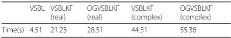
5.7 Example 7: the cost time versus different methods In addition, the computational time of different DOA tracking methods is also analyzed. We conduct an evaluation of the computational complexity using TIC and TOC instruction in MATLAB. All the simulation results are obtained using the same PC with an Intel i7-6700 and 8 GB RAM, running MATLAB 2015b on 64-bit Windows 10. The average computational time is given in Table 2, which is obtained from 300 Monte Carlo trials and 50 time intervals. It can be seen that the time cost of the proposed method is more than that of VSBL, but the precision of the pro-posed method is higher. Comparing VSBLKF with OGVSBLKF, we observe that the method based on the off-grid model only needs 7 s more than that based on the on-grid model, so the performance of OGVSBLKF is better. Note that the theoretic com-plexity is O(Tυ) approximately, υ is the iteration numbers. The reason of long cost time of the propose method is that using the Kalman filter embedded into the VSBL might increase the iteration numbers to avoid the local values.
Fig. 13RMSE as a function of SNR in the off-grid model
Fig. 14RMSE as a function of SNR in the off-grid model with different grid interval
Fig. 15Traces of three methods for two signals
Table 2Comparison of time cost for different methods
VSBL VSBLKF (real)
OGVSBLKF (real)
VSBLKF (complex)
OGVSBLKF (complex)
6 Conclusions
In order to track the 2-D DOAs, we construct the state transition function according to the TP model based on a spherical array. The angular space is divided into grids to model a sparse signal. Through combining VSBL and KF methods, we propose an effective method called VSBLKF to track dynamic DOAs, where the KF estima-tion is embedded into the VSBL to estimate the signals. Besides, we extend our algorithm to the off-grid model. Simulations show that the proposed method achieves better tracking and anti-noise performance than VSBL and KF. In the future, we will extend the algorithm to wideband signals.
Acknowledgements
The authors would like to thank the editor and anonymous reviewers for their valuable comments.
Funding
The work was supported by the National Natural Science Foundation (61571279, 61501288) and the Shanghai Science and Technology Commission Scientific Research Project (16010500100).
Authors’contributions
QH and JH designed and implemented the proposed algorithm and wrote the paper. KL and YF scientifically supervised the work and contributed in implementing the proposed algorithm. All authors read and approved the final manuscript.
Competing interests
The authors declare that they have no competing interests.
Publisher’s Note
Springer Nature remains neutral with regard to jurisdictional claims in published maps and institutional affiliations.
Received: 24 May 2017 Accepted: 15 March 2018
References
1. A Hassanien, SA Vorobyov, Transmit energy focusing for DOA estimation in MIMO radar with colocated antennas. IEEE Trans. Signal Process.59(6), 2669–2682 (2011)
2. H Krim, M Viberg, Two decades of array signal processing research: the parametric approach. IEEE Signal Process. Mag.13(4), 67–94 (1996) 3. A Boukerche, H Oliveira, E Nakamura, A Loureiro, Localization systems for
wireless sensor networks. IEEE Trans. Wirel. Commun.14(6), 6–12 (2007) 4. M Carlin, P Rocca, G Oliveri, Directions-of-arrival estimation through
Bayesian compressive sensing strategies. IEEE Trans. Antennas Propag.61(7), 3828–3838 (2013)
5. B Wang, J Liu, X Sun, Mixed sources localization based on sparse signal reconstruction. IEEE Signal Process. Lett.19(8), 487–490 (2012)
6. D Malioutov, M Cetin, A Willsky, A sparse signal reconstruction perspective for source localization with sensor arrays. IEEE Trans. Signal Process.53(8), 3010–3022 (2005)
7. D Wipf, B Rao, An empirical Bayesian strategy for solving the simultaneous sparse approximation problem. IEEE Trans. Signal Process.55(7), 3704–3716 (2007) 8. S Ji, Y Xue, L Carin, Bayesian compressive sensing. IEEE Trans. Image Process.
56(6), 2346–2356 (2008)
9. S Babacan, R Molina, A Katsaggelos, Bayesian compressive sensing using Laplace priors. IEEE Trans. Image Process.19(1), 53–63 (2010)
10. DP Wipf, BD Rao, An empirical Bayesian strategy for solving the simultaneous sparse approximation problem. IEEE Trans. Signal Process 55(7), 3704–3716 (2007)
11. SD Babacan, R Molina, AK Katsaggelos, Bayesian compressive sensing using Laplace priors. IEEE Trans. Image Process.19(1), 53–63 (2010)
12. JF Gu, SC Chan, WP Zhu, et al., Joint DOA estimation and source signal tracking with Kalman filtering and regularized QRD RLS algorithm. IEEE Trans Circuits. Syst. II, Exp Briefs60(1), 46–50 (2013)
13. B Yang, Projection approximation subspace tracking. IEEE Trans. Signal Process.43(1), 95–107 (Jan. 1995)
14. C Liu, G Wang, J Xin, et al., Low complexity subspace-based two-dimensional direction-of-arrivals tracking of multiple targets. Proc. ICSP, 1825–1829 (2012) 15. J Wu, J Xin, G Wang, et al., Two-dimensional direction tracking of coherent
signals with two parallel uniform linear arrays. Proc. ICSP, 183–187 (2012) 16. N Vaswani, J Zhan, Recursive recovery of sparse signal sequences from
compressive measurements: a review. IEEE Trans. Signal Process.64(13), 3523–3549 (2016)
17. N Vaswani, LS-CS-residual (LS-CS): compressive sensing on least squares residual. IEEE Trans. Signal Process.58(8), 4108–4120 (2010)
18. N Vaswani, W Lu, Modified-CS: modifying compressive sensing for problems with partially known support. IEEE Trans. Signal Process.58(9), 4595–4607 (2010) 19. M Friedlander, H Mansour, et al., Recovering compressively sampled signals using
partial support information. IEEE Trans. Inf. Theory58(2), 1122–1134 (2012) 20. W Lu, N Vaswani, Regularized modified BPDN for noisy sparse
reconstruction with partial erroneous support and signal value knowledge. IEEE Trans. Signal Process.60(1), 182–196 (2012)
21. XZ Gao et al., A sequential Bayesian algorithm for DOA tracking in time-varying environments. Chin. J. Electron.24(1), 140–145 (2015) 22. J Jia, L Yu, H Sun, et al., Dynamic DOA estimation via locally competitive
algorithm. Proc. ICSP, 336–340 (2014)
23. Higuchi, Takuya, et al. Underdetermined blind separation and tracking of moving sources based on DOA-HMM. IEEE Int. Conf. Acoust, Speech and Signal Process, 3191-3195 (2014).
24. Y Tian, Z Chen, F Yin, Distributed imm-unscented kalman filter for speaker tracking in microphone array networks. IEEE Trans. Audio Speech Language Process.23(10), 1637–1647 (2015)
25. P Khomchuk, I Bilik, Dynamic direction-of-arrival estimation via spatial compressive sensing. Proc. Radar, 1191–1196 (2010)
26. M Hawes, L Mihaylova, F Septier, et al., A Bayesian compressed sensing Kalman filter for direction of arrival estimation. Proc. IEEE Int. Conf. Inf. Fusion, 969–975 (2015)
27. F Ning, L Ning, et al., Combining compressive sensing with particle filter for tracking moving wideband sound sources. IEEE Int. Conf. Signal Process, Commun and Comput, 1–6 (2015)
28. B Rafaely, Analysis and design of spherical microphone arrays. IEEE Trans. Speech, Audio Process.13(1), 135–143 (2005)
29. Q Huang, T Wang, Acoustic source localization in mixed field using spherical microphone arrays. EURASIP J. Adv. Sign. Process.2014(1), 1–16 (2014) 30. R Goossens, H Rogier, 2-D angle estimation with spherical arrays for scalar
fields. Signal Process., IET3(3), 221–231 (2009)
31. H Sun, S Yan, U Svensson, Robust spherical microphone array beamforming with multi-beam-multi-null steering, and sidelobe control. in Proc. IEEE Workshop Appl. Signal Process. Audio Acoust, 113–116 (2009)
32. B. Rafaely, Fundamentals of Spherical Array Processing, Springer, chapter 1, pp. 10, 2015.
33. DA Linebarger, RD DeGroat, EM Dowling, Efficient direction-finding methods employing forward-backward averaging. IEEE Trans. Sign. Proc.42, 2136–2145 (1994)
34. A Roda, C Micheloni, Tracking sound sources by means of HMM. IEEE Int. Conf. Adv. Video and Signal-Based Surveillance, 83-85 (2011)
35. S Farahmand, GB Giannakis, G Leus, et al., Tracking target signal strengths on a grid using sparsity. Eurasip J. Adv. Sign. Proc.2014(1), 1–17 (2011) 36. C Bishop,Pattern recognition and machine learning(Springer-Verlag, New
York, 2008), pp. 477–482
37. MJ Wainwright, MI Jordan, Graphical models, exponential families, and variational inference. Now Publishers Inc, pp. 159–164, 2008 38. EP Xing, MI Jordan, S Russell, A generalized mean field algorithm for
variational inference in exponential families. Proceed. Conf. Uncertainty Artific. Intel, 583–591 (2012)
39. DG Tzikas, AC Likas, NP Galatsanos, The variational approximation for Bayesian inference. IEEE Sign. Proc. Magazine.25(6), 131–146 (2008) 40. P. Sebah, X. Gourdon,“Introduction to the Gamma Function,”[Online].
Available:http://www.csie.ntu.edu.tw/~b89089/link/gammaFunction.pdf. 41. Z Yang, L Xie, C Zhang, Off-grid direction of arrival estimation using sparse