Using TNT NN to unlock the fast full spatial inversion of large magnetic microscopy data sets

FULL PAPER

Using TNT-NN to unlock the fast full spatial

inversion of large magnetic microscopy data

sets

Joseph M. Myre

_{, Ioan Lascu}

_{, Eduardo A. Lima}

_{, Joshua M. Feinberg}

_{, Martin O. Saar}

and Benjamin P. Weiss

Abstract

Modern magnetic microscopy (MM) provides high-resolution, ultra-high-sensitivity moment magnetometry, with the ability to measure at spatial resolutions better than 10−4 m and to detect magnetic moments weaker than 10−15 Am2 . These characteristics make modern MM devices capable of particularly high-resolution analysis of the magnetic properties of materials, but generate extremely large data sets. Many studies utilizing MM attempt to solve an inverse problem to determine the magnitude of the magnetic moments that produce the measured component of the magnetic field. Fast Fourier techniques in the frequency domain and non-negative least-squares (NNLS) methods in the spatial domain are the two most frequently used methods to solve this inverse problem. Although extremely fast, Fourier techniques can produce solutions that violate the non-negativity of moments constraint. Inversions in the spatial domain do not violate non-negativity constraints, but the execution times of standard NNLS solvers (the Lawson and Hanson method and Matlab’s lsqlin) prohibit spatial domain inversions from operating at the full spatial resolution of an MM. In this paper, we present the applicability of the TNT-NN algorithm, a newly developed NNLS active set method, as a means to directly address the NNLS routine hindering existing spatial domain inversion meth-ods. The TNT-NN algorithm enhances the performance of spatial domain inversions by accelerating the core NNLS routine. Using a conventional computing system, we show that the TNT-NN algorithm produces solutions with residu-als comparable to conventional methods while reducing execution time of spatial domain inversions from months to hours or less. Using isothermal remanent magnetization measurements of multiple synthetic and natural samples, we show that the capabilities of the TNT-NN algorithm allow scans with sizes that made them previously inaccesible to NNLS techniques to be inverted. Ultimately, the TNT-NN algorithm enables spatial domain inversions of MM data on an accelerated timescale that renders spatial domain analyses for modern MM studies practical. In particular, this new technique enables MM experiments that would have required an impractical amount of inversion time such as high-resolution stepwise magnetization and demagnetization and 3-dimensional inversions.

Keywords: Magnetic microscopy, Rock magnetism, Non-negative least-squares

© The Author(s) 2019. This article is distributed under the terms of the Creative Commons Attribution 4.0 International License (http://creat iveco mmons .org/licen ses/by/4.0/), which permits unrestricted use, distribution, and reproduction in any medium, provided you give appropriate credit to the original author(s) and the source, provide a link to the Creative Commons license, and indicate if changes were made.

Open Access

*Correspondence: [email protected]

1 _{Department of Computer and Information Sciences, University of St.} Thomas, 2115 Summit Ave., Saint Paul, MN 55105, USA

Introduction

Modern magnetic microscopes (MMs) have been devel-oped to analyze the microscale natural remanent mag-netization and rock magnetic properties of rocks and minerals (Harrison and Feinberg 2009) and are capable of high-resolution, high-sensitivity measurements on geologic samples (Weiss et al. 2007b). MMs encompass superconducting quantum interference device (SQUID), magnetic tunnel junction (MTJ), giant magnetoresist-ance (GMR) sensors, and quantum diamond microscopes (QDMs). MMs are capable of measuring samples with magnetic moments weaker than 10−15  Am2 (Fong et  al. 2005; Weiss et al. 2007a; Oda et al. 2016; Lima and Weiss 2016) at spatial resolutions on the order of micrometers (Liu et al. 2002; Liu and Xiao 2003; Liu et al. 2006; Hank-ard et al. 2009; Lima et al. 2014; Glenn et al. 2017).

MM has been applied to investigations of ultrafine-scale magnetostratigraphy (Oda et  al. 2011; Noguchi et al. 2017a), shock remanent magnetization (Gattacceca et al. 2006, 2010), rock magnetism (Hankard et al. 2009; Kletetschka et  al. 2013), studies of nebular magnetism using chondrules (Fu et al. 2014), and the paleointensity of the magnetic field of Earth (Weiss et al. 2007a; Fu et al. 2017; Weiss et al. 2018) and Mars (Weiss et al. 2008). The high-resolution capability of MMs can yield extremely large data sets. Analyzing these data sets is dominated by solving an inversion problem, which obtains the distribu-tion of magnetic sources from the measured magnetic field. As with mapping of magnetic fields of magnetiza-tion, retrieving magnetization from magnetic fields is non-unique without the use of other constraints and can be computationally expensive (Weiss et al. 2007b; Lima and Weiss 2016).

Weiss et al. (2007b) describe three formulations of the least-squares inversion problem to obtain the magnetic sources of a sample from MM magnetic field measure-ments: unrestricted, unidirectional, and uniform. Unre-stricted solutions obtain the three vector components of Q dipoles at fixed positions within the sample from P

measurements of the vertical (z) component of the mag-netic field. Obtaining a solution at the full resolution of the scan necessitates solving an underdetermined linear least-squares problem with an infinite number of possible solutions. This type of solution is typically appropriate for scans of unidirectional natural remanent magneti-zation (NRM). Unidirectional solutions determine the magnitudes of Q dipoles at fixed positions within the sample from P measurements of the z-component of the magnetic field. For a full resolution solution, this requires solving a linear least-squares problem. This problem is well determined as all of the dipole orientations are fixed in any one direction (described by the angles θ and φ in spherical coordinates), but their magnitudes are allowed

to vary independently. Because all dipoles share an ori-entation, it is reasonable to impose a non-negativity constraint to all dipoles once all dipoles share a posi-tive orientation. To solve numerical problems with such a constraint, it is natural to use a non-negative least-squares (NNLS) solver. This type of solution is typi-cally most applicable for scans of saturation isothermal remanent magnetization (SIRM). Solutions provided by NNLS are naturally smooth and should be regarded as approximations of the true physical system (a common stance in numerical modeling). This is particularly true if some dipoles remain in the “negative” orientation or are misaligned relative to the primary orientation after the sample acquires an SIRM due to sample anisotropy or interactions between remanence carriers. In such a case, those dipoles in the unidirectional solution would be constrained to zero or approximated to their compo-nent in the SIRM orientation. The more a sample vio-lates the unidirectionality and positivity assumptions of the unidirectional inversion, the more the solution can be regarded as an approximation. Uniform solutions are obtained by requiring all dipole orientations and magni-tudes to be identical. This gives rise to a problem with P

measurements of the z-component of the magnetic field and only three unknowns. For MM data, this is often severely overdetermined.

samples from single component measurements. Lima et  al. (2013) improved upon this work by regularizing the inverse problem, dampening noise, and enhancing processing speed.

An unavoidable consequence of applying Fourier tech-niques to SIRM data (to obtain a unidirectional solution) is the potential violation of non-negativity constraints. A typical method to handle Fourier solution components that violate non-negativity is to threshold those variables to zero. This can yield solutions that are not smooth and may not be physically valid. Because Fourier techniques operate in the frequency domain, it can be difficult to impose solution constraints that are related to the spatial domain. Such a constraint could be as simple as restrict-ing valid solution variables to the spatial domain of a sample.

Weiss et  al. (2007b) developed the first spatial inver-sion technique capable of producing unique solutions composed of three component magnetic distributions. This technique uses the equivalent source formalism (Dampney 1969; Emilia 1973) to represent the inverse problem in a least-squares manner. Specifically, the unre-stricted solution can be obtained via unconstrained least-squares and the unidirectional and uniform solutions are obtained by NNLS. The uniform problem is typically extremely overdetermined for MM data and can be sidered relatively simple to solve computationally. In con-trast, the unrestricted and unidirectional problems can be computationally challenging. Because the unrestricted problems are underdetermined, they are not guaranteed to be unique without additional constraints. All other factors being equal, unidirectional problems are smaller than unrestricted problems by a factor of ∼  3 because the orientation is known and only the determination of dipole magnitudes remain. Unidirectional problems are also well-determined, which allows a unique solution to be obtained. Despite these positive characteristics, unidi-rectional problems can necessitate a significant amount of computational work due to the quantity of data acquired by the high-resolution of MM devices.

Addressing the NNLS problem within the unidirec-tional formulation has proven to be computaunidirec-tionally expensive, requiring two months of computation time to produce a solution for the inversion of a single sam-ple (Weiss et al. 2007b). A number of modifications were made to the computational approach to attain tractable computation for NNLS methods, with each modifica-tion imposing some degree of undesirable consequences regarding the resulting inverse solution. Although the continuous increase in the speed of modern computers diminishes the necessity of these modifications when solving the original inversions of Weiss et  al. (2007b), improvements in high-resolution magnetism acquisition

yield continuously larger data sets which keep these modifications relevant.

For example, a second pseudo-spatial technique, developed by Usui et  al. (2012), blends spatially local-ized Backus–Gilbert averaging kernels (Backus and Gilbert 1968) with the subtractive optimally localized averages (SOLA) method (Pijpers and Thompson 1992). The Usui et al. (2012) approach avoids the high compu-tational requirements of the spatial inversion technique of Weiss et  al. (2007b) by performing some significant computation in the frequency domain. Specifically, it approximates a matrix inversion with a periodic bound-ary approximation and FFT. In some cases, this style of pseudo-spatial method has been shown to be almost as fast as methods that operate purely in the frequency domain (Pijpers 1999). Further, Pijpers (1999) shows that the spatial resolution of the SOLA method can approach that of the acquisition device. However, Usui et al. (2012) state that the shape of their averaging ker-nels used to invert geologic data suggest a spatial reso-lution of ∼ 1 mm. In fact, Usui et al. (2012) successfully produced magnetization models with a spatial resolution of ∼ 1 mm. For MMs to obtain well resolved field meas-urements, the spatial resolution of MM spatial inversion solutions are limited to approximately half the sensor-to-sample distance. Considering this limitation, the spatial resolution of most published MM data is on the order of 0.1 to 0.15 mm or less.

Ultimately, determining the effective spatial resolu-tion of an inversion of MM data is a complex problem (Lima et  al. 2006). Several factors affect spatial resolu-tion (e.g., sensor-to-sample distance, sensor active area/ volume, signal-to-noise ratio, mapping step size, regular-ization strategy used), which make comparison of inver-sion methods delicate, particularly when evaluating data obtained using different MM systems. Thorough discus-sions of the relationships between these factors are pro-vided by Chatraphorn et  al. (2002); Fleet et  al. (2001); Lima et  al. (2006, 2014); Lima and Weiss (2016); Oda et al. (2016); Egli and Heller (2000), and Roth and Wik-swo Jr (1990).

The fundamental goal of any scheme for inverting MM data is to quickly determine the magnetic sources within the entire spatial domain of the sample without reduc-ing resolution. Existreduc-ing methods have had to make com-promises on speed, resolution, sample completeness, or physical validity, thereby hindering the full capabili-ties of the inversion method. In this paper, we focus on the NNLS problem at the heart of unidirectional spatial inversion, as it provides an excellent avenue toward high-resolution unique solutions.

large problems, to the inversion of real-world MM data, using the unidirectional inversion technique of Weiss et  al. (2007b). Active set NNLS algorithms share the idea of constructing an “active set” of variables that are fixed at zero to not violate the non-negativity constraint. TNT-NN is an active set NNLS algorithm that exhib-its significant performance enhancement over previous active set algorithms. These enhancements are primarily enabled by two means: (1) by improving the construction of the active set and (2) by enhancing the method used to solve the core least-squares problem. Through the use of TNT-NN to solve the core NNLS problem, the inver-sion scheme of Weiss et al. (2007b) can be applied to MM data using the spatial resolution of the MM device, with-out the need to compromise the physical validity of the inverse solutions.

The TNT-NN algorithm is used to obtain the magnetic sources of four samples; a synthetically magnetized Uni-versity of Minnesota logo, a 30 µ m thin section of basalt from the Mauna Loa volcano (Weiss et  al. 2007a, b), a 30–60 µ m thin section of ferromanganese crust (Noguchi et al. 2017a), and a 100 µ m thin section of a speleothem from Spring Valley Caverns in South East Minnesota, USA (Dasgupta et al. 2010). We show that the TNT-NN algorithm is a suitable update to the spatial inversion technique developed by Weiss et  al. (2007b) due to its enhanced performance and numerical accuracy.

Existing computational roadblocks and circumvention efforts

Investigating existing least-squares techniques to analyze MM data reveals two hurdles with undesirable conse-quences: extremely large data sets and inefficient solv-ers for the core non-negative least-squares problem. Strategies to overcome these hurdles are outlined in the remainder of this Section.

Large data sets

The spatial resolution of MMs enables a high number of scanning measurements to be made for a given sample area, resulting in the generation of large data sets. For example, a 35 mm × 35 mm area, scanned with a 100 µ m resolution, produces 122,500 measurements.

A well-determined problem, consisting of 106 elements

(1000 ×  1000) does not typically present a significant

computational challenge. However, in the NNLS prob-lem, the spatial least-squares inversions are analyzing magnetic data that require the construction of the inter-action (Jacobian) matrix for the entire scanned area. This quickly increases the problem size for non-trivial (non-uniform) inverse problems, so that a scan producing 105 elements yields a 105×105 ( 1010 element) Jacobian

matrix. A Jacobian matrix of this scale can have storage

requirements approaching 100  GB. Attempting to per-form mathematical operations on such large matrices with a typical desktop computer often causes a phenom-enon known as thrashing (Denning 1968). Thrashing is the inability to store the entirety of a data buffer within fast access memory, causing repeated data transfers with larger capacities but slower memory access. The over-head caused by data transfer leaves the processor unable to perform useful computation due to data starvation. This effectively reduces the performance of the computer system to that of the slower memory, which acts as a bot-tleneck. Contemporary computer systems have approxi-mately a six order of magnitude difference in access time between typical RAM (on the order of 10−9 s) and hard disk drive (on the order of 10−3 s) systems.

Because the Jacobian matrices created during the spa-tial inversion process have significant memory require-ments, it has thus far been necessary to implement computational strategies to avoid thrashing. These strate-gies include specimen division and dipole thresholding. Both are methods for reducing the size of the data set used in the MM inversion problem, with the secondary effect of creating a smaller core least-squares problem that reduces the time needed to find a solution. Unfor-tunately, both strategies produce approximations of the solution.

Specimen subdivision splits the MM measurements into subsections. The inversion of the sample is then performed by inverting the subsections separately. With sufficiently small divisions, the overall memory require-ments of the Jacobian matrix are reduced to the point where thrashing is minimized. Solving these subsections is also more computationally tractable than for the sam-ple as a whole due to the reduction in overall variables. By subdividing the sample and finding the inverse solution of each subdivision separately, the magnetic interactions between subsections are ignored. Consequently, this method violates the mathematical theory of the inversion problem, which requires that the spatial domain of the magnetic sources within a sample to be finite and fully encapsulated by the inversion problem domain (compact support) to ensure a unique solution (Baratchart et  al. 2013; Lima et al. 2013).

the field at the boundary that is not incorporated when using specimen subdivision to achieve computational tractability.

Thresholding the long range interactions of each dipole allows interactions that fall below a specified threshold to be withheld from computation. Excluding other dipoles from consideration means that their associated entries in the Jacobian matrix are fixed at zero. Inversion meth-ods for large data sets from satellite magnetic fields com-monly apply this type of thresholding (Purucker et  al. 1996).

Dipole interaction thresholding was applied by Weiss et  al. (2007b) to form a sparse approximation of the Jacobian, A, as A† . By creating a sparse approximation, A† , overall data storage requirements are reduced. This

reduction scales with the degree of sparsity of A† . The

computation of A† is accelerated compared to the

com-putation of A since A† effectively reduces the problem

size and allows sparse methods to be used. The reduction in computation time to form A† also reduces the overall

computation time for uniform inverse solutions, which are dominated by the computation of A.

The ability to use sparse matrix methods offers an alluring reason to use A† in lieu of A. Weiss et al. (2007b)

exploit sparse methods and solve A† using the more

com-putationally efficient lsqlin function in Matlab, which uses a preconditioned conjugate gradient routine at its core, instead of the lsqnonneg NNLS function for dense problems. However, the solutions obtained using A† are

approximate solutions, just as A† is an approximation of A.

Inefficient active set least‑squares solvers

The core of the MM unidirectional and uniform inversion routines is an NNLS solver. The primary Matlab NNLS solver (lsqnonneg) is implemented using the seminal 1974 Lawson and Hanson NNLS (LH-NNLS) algorithm (Law-son and Han(Law-son 1995). The LH-NNLS algorithm can eas-ily be considered the most widely used NNLS algorithm as it is consistently provided by popular software pack-ages, including the widely used computer algebra system Matlab, GNU R (Mullen and van Stokkum 2012), and scientific tools for Python (scipy) (Jones et  al. 2001). It is also repeatedly encountered in the reference literature as the recommended method for solving non-negative least-squares problems (Aster et  al. 2011; Parker 1994; Xiong and Kirsch 1992).

The LH-NNLS algorithm is an active set strategy that attempts to find solutions to the NNLS prob-lem. This constrained NNLS problem can be stated as

minx||Ax−b||2, such thatx≥0 , where A is the m×n

system of equations, b is the solution vector of measured

data, and x is the vector of obtained parameters that min-imizes the L 2_{-norm of the residual.}

The LH-NNLS algorithm determines constrained vari-ables by iterating through the set of varivari-ables one at a time, which commonly results in slow convergence. The Fast NNLS (FNNLS) algorithm developed by Bro and De Jong (1997) improves upon the LH-NNLS algorithm by avoiding redundant computations and allowing the programmer to load an initial active set of constrained variables. Using small real and synthetic test suites, Bro and De Jong report that FNNLS reduces execution time compared to NNLS by factors of 2–5.

Recently, graphics processing units (GPUs) have been exploited as high performance computing devices (Walsh et al. 2009) to improve runtime performance over CPU implementations of the LH-NNLS algorithm (Luo and Duraiswami 2011). Like CPU algorithms, the problem size that the GPU algorithm is capable of solving is lim-ited by the available memory. The amount of memory available on contemporary GPUs is fixed and typically less than 10GB. This is a fraction of the memory space that is required for the inversion of MM data (which can easily surpass 100  GB). Recent GPU technology from NVIDIA enables the GPU to operate on data stored in host memory. However, operating on data in host mem-ory, external to the GPU, incurs a significant performance penalty, similar to thrashing, due to additional access and transfer time.

Overcoming computational roadblocks

Storing large data sets

Thrashing between main memory and hard disk storage can easily be avoided by using a computer system with sufficient main memory to meet the storage require-ments of the data set of interest. Desktop computers with sufficient memory to avoid thrashing when handling sys-tems of this size are somewhat rare, but they are not out of reach for the majority of researchers. A contemporary computer built to handle the largest MM data sets pre-sented in this paper would cost less than $10,000 (USD) and would not require any special training. Computing resources of this nature are commonly available at the computational centers of many research institutions.

A new non‑negative least‑squares algorithm: TNT‑NN

Due to the convexity (i.e., a local minimum must be a global minimum) of the least-squares objective function (Boyd and Vandenberghe 2004) the TNT-NN algorithm can take an “algorithmic license” to guess what variables compose the active set without the risk of becoming locked into a local minimum. The suitability of the vari-ables is determined by ranking them by their gradients (their change between iterations). Those variables with the largest positive gradients are tested by moving them into the unconstrained set first. This allows the active set to be modified by a large amount of variables in a single iteration. In contrast, other common active set methods typically modify the active set by a single variable per iteration (Lawson and Hanson 1995; Bro and De  Jong 1997). The ability to modify the active set by many vari-ables in a single iteration allows the TNT-NN algorithm to reduce the total number of iterations necessary for convergence.

In active set methods, solving the core unconstrained least-squares problem is independent from the con-struction of the active set. To accelerate the core uncon-strained least-squares solver, Myre et al. (2018) developed the TNT algorithm. The TNT algorithm implements the Cholesky factor of the normal equations as a precondi-tioner to a left-preconditioned conjugate gradient normal residual (PCGNR) method (Saad 2003). PCGNR can be thought of as a computationally cheap mechanism that iteratively improves the solution. The normal equations are explicitly formed to create the preconditioner for CGNR. The numerical issues typically associated with the normal equations and the condition number of the problem are thereby avoided.

The condition number of a matrix A , _κ(A₎ , is the ratio of the largest to the smallest singular values of A and it can be used as indicator of numerical inaccuracies in solutions (Cline et al. 1979). A numerical “rule of thumb” states that when solving a system of equations, Ax₌b ,

“one must always expect to lose log10κ(A) digits in com-puting the solution” (Trefethen and Bau  III 1997, Lec. 12). The normal equations are particularly susceptible to this issue as κ(ATA)=κ(A)2 . TNT only explicitly forms

the normal equations to generate the preconditioner. Myre et  al. (2018) show that TNT obtains solutions two to sixteen times faster than other conventional solv-ers and that TNT consistently produces solutions where the L 2_{-norm of the solution residual is on the order of}

10−15 for ill-conditioned problems ( _{κ >}

=108 ) and 10−28

for well-conditioned problems ( κ <108 ). For

well-deter-mined and well-conditioned problems, the L 2_{-norm of} the TNT solution residual is always less than or equal to those of alternative methods while also decreasing execu-tion time in the majority of tests.

Using TNT as the core unconstrained least-squares solver, TNT-NN likewise yields solutions where the L 2 -norm of the solution residual is always less than or equal to those of alternative methods for well- and overde-termined and well-conditioned problems. Myre et  al.

(2017a) show that with TNT, TNT-NN can outperform

the execution time performance of the relatively more modern FNNLS method by up to a factor of 180 when solving small systems up to 25000×25000 and by more

than 40 times when solving a larger ( 45000×45000 )

system.

Application to synthetic and natural samples

We compare the least-squares inversions of MM scans of four samples using LH-NNLS, lsqlin, and TNT-NN. We restrict our comparisons to results obtained using LH-NNLS and lsqlin as all previously reported spatial inver-sion results have been obtained using these methods.

Comparing TNT-NN to LH-NNLS could be consid-ered unfair due to the age of the LH-NNLS algorithm. We consider the comparison necessary as LH-NNLS is the routine that is most consistently used throughout other published spatial inversions that do not circumvent the computational hurdles described earlier.

We analyze the spatial least-squares inversion solu-tions of one synthetic and three natural samples: a syn-thetic University of Minnesota (UMN) logo, a 30 µ m thin section of basalt from the Mauna Loa volcano (Weiss et  al. 2007a, b), a 30–60 µ m thin section of ferroman-ganese crust from the Takuyo–Daigo Seamount (Nogu-chi et al. 2017a), and a 100 µ m thin section of a calcite speleothem from Spring Valley Caverns in South East Minnesota, USA (Dasgupta et  al. 2010). The synthetic UMN logo inversion is small enough to be solved using LH-NNLS and TNT-NN. The basalt thin section inver-sions are solved using lsqlin (combined with sample sub-division) and TNT-NN. LH-NNLS is prohibitively slow for solving anything that is significantly larger than the synthetic UMN MM scan. The ferromanganese crust and speleothem MM data are large enough to be considered intractable for the LH-NNLS and lsqlin methods with-out significant modification. As such, only the TNT-NN method is used to perform these inversions.

Although we vary the spatial resolution of the NNLS solutions across these samples, we restrict the best pos-sible spatial resolution to half the sensor-to-sample distance. This allows the NNLS method to obtain well resolved sources without inducing instabilities. This constraint is solely due to the physics of the problem being solved. On its own, NNLS has no inherent spatial constraints.

Each real-world sample presented here is composed of data from a single MM scan. We then use different numerical methods to invert the scan (or alternatively, a cropped region of the scan). As differences between MM devices and scanning conditions can yield different spa-tial resolutions, we do not make direct comparisons of inversions result quality between different samples.

All inversions (using LH-NNLS, lsqlin and TNT-NN) were performed using Matlab 2017b and a single com-pute node on the Mesabi supercomcom-puter at the Min-nesota Supercomputing Institute. This compute node consists of dual 12 core Intel Haswell E5-2680v3 pro-cessors at 2.5 GHz with up to 1 TB of memory. None of the analyses presented in this paper require more than 365 GB of memory. Comparable computing systems are available at most computing centers or easily purchased for $10,000 (USD) or less.

For each sample, the performance of each technique is compared in terms of execution time and the root mean square (RMS) of the solution residual. We also examine the calculated bulk magnetic moments of the solutions for these samples. In all cases the bulk magnetic moment is calculated as the sum of the ( θ , φ ) component of all solution dipoles. In the synthetic UMN logo case, we compare the calculated moment to the known moment. For the natural samples, we compare the calculated moments to experimentally measured moments.

Synthetic UMN logo

The use of simple alphanumeric characters, simple sym-bols, and institutional logos as baselines for numerical experimentation is common practice (Baratchart et  al. 2013; Egli and Heller 2000; Lima et  al. 2006; Lima and Weiss 2009; Lima et al. 2013) as these synthetic data sets often represent worst-case scenarios when testing new methods. In particular, synthetic samples of this nature allow the inverse solution to be exactly known which enables an examination of how robust the inversion method is when solving problems of varying difficulty. MM data for this synthetic sample are created numeri-cally using Matlab R2017a. Originally presented by Myre et al. (2017a), the process starts by generating a synthetic 2-dimensional magnetic source map. An image is treated as a discretized set of square magnetic sources from which magnetic field maps are calculated. The synthetic

MM scan is then obtained as the vertical component of the magnetic field, Bz , at a height, h, above the syn-thetically created and irregularly shaped set of magnetic sources.

We created a synthetic saturation isothermal remanent magnetization (SIRM) scan of the UMN logo by convert-ing a 67×50 pixel grayscale image of the UMN logo to

a magnetic source map. By introducing negative values in the image, the final synthetic SIRM sample will have points roughly mimicking magnetic sources that have failed to align with the saturating field.

By imposing a non-negativity constraint on such sources, the solution to the inversion problem is a unique distribution of magnetic sources [the unidirectional problem (Weiss et  al. 2007b; Baratchart et  al. 2013)]. Without the non-negativity constraint, the solutions to the inversion problem to obtain the magnetic sources are non-unique [the unrestricted problem (Weiss et  al. 2007b; Baratchart et al. 2013)]. In fact, any magnetic field map can be modeled by unidirectional sources without the non-negativity (also known as unidimensional) con-straint (Baratchart et al. 2013).

The following is an outline of the process used to cre-ate the synthetic SIRM scan of the UMN logo. The values in the original grayscale image range from 0 to 255. To create the set of magnetic sources requiring the appli-cation of the non-negativity constraint, we multiply the few grayscale values less than 75 by −1 . Those grayscale

values in the image less than 75 correspond to relatively low-intensity background shading pixels in the origi-nal image. All of the values are then scaled such that the maximum value of the logo is 4.3233×10−11 , and the minimum value of the logo is −1.4788×10−12 , which is in the typical range of magnetization intensity for natu-ral samples measured in Am2 _{. All orientations are in the} ±z-direction (i.e., in or out of the page), where the sign of the converted grayscale value determines the orientation in the z-direction. These new pixel values are then treated as magnetic sources (each source is 100×100µm2 for this synthetic sample) and used to calculate the vertical component of the magnetic field, Bz , at a height, h above the synthetic magnetic sources.

the simulated synthetic UMN logo with negativity con-straint violations and Gaussian white noise corruption using LH-NNLS and TNT-NN, (5) solving the simulated synthetic UMN logo with higher magnitude negativity constraint violations using LH-NNLS and TNT-NN, (6) solving the simulated synthetic UMN logo with higher magnitude negativity constraint violations and Gaussian white noise corruption using LH-NNLS and TNT-NN. All solutions obtain dipoles oriented out of page, e.g., (0◦ ,

0 ◦ ) in ( _θ , _φ ). The known synthetic magnetic source

distri-butions for these scenarios are shown in Fig. 1.

In scenarios where the simulated MM scan is cor-rupted by Gaussian white noise (2, 4, and 6), we measure the amount of signal degradation using the signal-to-noise Ratio (SNR) reported in decibels (dB) as

where σ_signal2 is the variance of the (noiseless) synthetic B z field and σ_noise2 is the variance of the noise. For scenarios incorporating noise, we use an SNR of 40 dB.

For scenarios 1 and 2, we modify our original syn-thetic SIRM creation procedure to ensure no violations of the non-negativity constraint. We do this by taking the absolute value of the original synthetic SIRM mag-netic source map. For scenarios 5 and 6, we modify our original synthetic SIRM creation procedure to create more, and higher magnitude, negativity constraint viola-tions (relative to scenarios 3 and 4). We do this by first switching all values in the original grayscale image from 1 to 45 from positive to negative. We then scale the nega-tive values of the logo to such that the minimum value is −7.55×10−12 and scale the positive values such that the maximum value is 4.3233×10−11 . Like the synthetic sources created for scenarios 3 and 4, the values obtained in the modified magnetic source maps are in the typi-cal range of magnetization intensity for natural samples measured in Am2 _{. The modified magnetic source maps}

(1)

are then used to calculate the simulated MM scans of the B z field.

We report the magnetic moment, the residual RMS, and error of each solution in Table 1. The solution error

Fig. 1 Known magnetic source distributions for scenarios 1 and 2 (a), scenarios 3 and 4 (b), and scenarios 5 and 6 (c). Note the nonlinear colorbar spacing in b and c. The field of view for each image is 6.7 mm × 5 mm, dipole orientation is out of page, and units are Am

2

for all images

Table 1 Summary of  the  unidirectional synthetic UMN logo inversion results

The first column shows the methods used to obtain the magnetic source distribution. The second column shows the scenario with which the results are associated. The third column lists the moment, m. The fourth column provides the residual RMS of the NNLS fits with the B z field. The final column reports the error of the NNLS solution relative to the known solution

Method Scenario m (Am2_{) Residual RMS}

is calculated as the L 2_{-norm of the difference between} the known magnetic source distribution and the mag-netic source distribution obtained as the inverse solution. As seen in Table 1, these measures are identical for LH-NNLS and TNT-NN.

For all scenarios of these synthetic MM scans, the inverse solutions produced by each method are similar and are a good visual match to the known solutions, as seen in Figs. 2, 3, and 4. Any differences between LH-NNLS and TNT-NN can be attributed to numerical noise, which typically becomes an issue when comput-ing with values near or below the machine epsilon, which is 2−53 (approximately _1.11

×10−16 ) on a computer using IEEE 754 double precision floating point numbers (Higham 2002).

The synthetic samples created with this method pre-sent an algorithmic “worst-case scenario” as the correct solution is a piecewise step function with sharp discon-tinuities. Any method that minimizes the L2-norm, like

least-squares, will act as a smoothing low-pass filter and spread out the solution in space. This leads to the crea-tion of nonphysical sources in the solucrea-tion. These sources can artificially inflate the net magnetic moment of the solution. This can be seen in the results from all scenar-ios in Table 1, where the LH-NNLS and TNT-NN solu-tions produce higher magnetic moments than that of the known solution.

Figure 2 shows results from scenarios 1 and 2. Both methods quickly produce solutions to scenario 1 with errors nine orders of magnitude below the machine epsi-lon. Scenario 1 is computationally attractive as the NNLS solvers should terminate in a single iteration with a valid solution (e.g., there are no variables requiring constraint). The addition of noise in scenario 2 introduces variables that violate the non-negativity constraint. This incurs additional NNLS solver iterations to obtain a valid solu-tion. The noise also causes nonphysical magnetic sources to be obtained in the least-squares solutions. These non-physical sources increase the magnetic moment, residual RMS, and error of the solutions.

Figure 3 shows results from scenarios 3 and 4. The introduction of noise in scenario 4 causes nonphysi-cal magnetic sources to be obtained in the least-squares solutions. These nonphysical sources slightly increase the magnetic moment, residual RMS, and error of the solutions.

Figure 4 shows results from scenarios 5 and 6. Enhanc-ing negativity causes a correspondEnhanc-ing enhancement of the difference between the known and obtained magnetic moment. The introduction of noise in scenario 6 does not have the same effect seen in scenario 4. Nonphysical magnetic sources are still obtained in the least-squares solutions, but these are much smaller in magnitude as the

magnitude of the primary solution dipoles is enhanced to compensate for the enhanced negativity. The balance between noise and negativity yields a negligible differ-ence in magnetic moment, residual RMS, and error of the solutions obtained by LH-NNLS and TNT-NN.

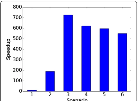
The performance of these two methods diverges when considering the amount of execution time necessary for each to obtain a solution. The multiplicative factor of improvement in execution time for TNT-NN relative LH-NNLS is shown in Fig. 5, reported as speedup (Lilja 2000, Ch. 2.5). We calculate speedup as

where exec(LH-NNLS) is the LH-NNLS execution time

and exec(TNT-NN) is the TNT-NN execution time.

The degree to which TNT-NN enhances performance over LH-NNLS is dependent on many factors, some of which include problem size, number of constraints, and condition number. The results in Fig. 5 show that, on average, TNT-NN provides a 623-fold improvement in execution time for the synthetic UMN logo scenarios with sample variables requiring constraint (scenarios 3–6). Restated, TNT-NN is capable of reducing 1  h of LH-NNLS computation time for synthetic MM inversion problems to approximately 5.78 s, on average.

Hawaiian basalt

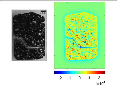
This 30 µ m thin section of tholeiitic basalt was collected from the Hawaiian Scientific Drilling Project (HSDP) 2 core through the Mauna Kea Volcano, Hawaii. These MM data were collected using the scanning SQUID micro-scope at the MIT Paleomagnetism Laboratory. The bulk moment of the sample was also measured using a 2G Enterprises 755 Rock Magnetometer in the same labora-tory. Collection and composition details for this sample, as well as the experimental conditions used to obtain the MM data, are provided by Weiss et al. (2007b).

Weiss et al. (2007b) measured the NRM and SIRM of this basalt thin section. To obtain unidirectional inverse solutions in a timely manner, it was found necessary to crop the spatial domain to a 13.6 mm × 19.1 mm region

around the sample and apply dipole thresholding to exploit sparse matrix techniques using the lsqlin routine, reducing computation time to several weeks. Further reductions in execution time required the use of sample subdivision to perform piecewise inversions.

We restrict our numerical analyses to the SIRM measurements of this sample (Fig. 6), using lsqlin and TNT-NN. Due to the prohibitive performance of the

lsqlin method, we restrict our lsqlin analyses to two scenarios at full measurement resolution (dipole spac-ing of 100 µm): (1) a piecewise scenario where five

(2) speedup=

Fig. 2 Comparison of SIRM magnetic sources for synthetic MM data of the UMN logo for scenarios 1 (a–f) and 2 (g–l): a, g simulated synthetic SIRM B z field in nT calculated from the UMN logo, b, h inverted magnetic sources from the TNT-NN method, c, i inverted magnetic sources from the LH-NNLS method, d, j known magnetic sources used to produce the synthetic MM scan (negative values are difficult to discern as their magnitudes are approximately an order of magnitude less than the positive values), e, k difference between the TNT-NN and known solutions, f, l difference between the LH-NNLS and known solutions. The field of view for each image is 6.7 mm × 5 mm, dipole orientation is out of page, and the units of

Fig. 3 Comparison of SIRM magnetic sources for synthetic MM data of the UMN logo for scenarios 3 (a–f) and 4 (g–l): a, g simulated synthetic SIRM B z field in nT calculated from the UMN logo, b, h inverted magnetic sources from the TNT-NN method, c, i inverted magnetic sources from the LH-NNLS method, d, j known magnetic sources used to produce the synthetic MM scan (negative values are difficult to discern as their magnitudes are approximately an order of magnitude less than the positive values), e, k difference between the TNT-NN and known solutions, f, l difference between the LH-NNLS and known solutions. The field of view for each image is 6.7 mm × 5 mm, dipole orientation is out of page, and the units of

Fig. 4 Comparison of SIRM magnetic sources for synthetic MM data of the UMN logo for scenarios 5 (a–f) and 6 (g–l): a, g simulated synthetic SIRM B z field in nT calculated from the UMN logo, b, h inverted magnetic sources from the TNT-NN method, c, i inverted magnetic sources from the LH-NNLS method, d, j known magnetic sources used to produce the synthetic MM scan (negative values are difficult to discern as their magnitudes are approximately an order of magnitude less than the positive values), e, k difference between the TNT-NN and known solutions, f, l difference between the LH-NNLS and known solutions. The field of view for each image is 6.7 mm × 5 mm, dipole orientation is out of page, and the units of

equally sized horizontal subdivisions (approximately 13.6  mm ×  4.3  mm) are solved independently and (2)

using the same 13.6  mm ×  19.1  mm cropped region

used by Weiss et  al. Using TNT-NN we address two scenarios at full measurement resolution (dipole spac-ing of 100 µm): (1) the same 13.6  mm ×  19.1  mm

cropped region used by Weiss et  al.and (2) using the full 19.0 mm × 25.0 mm measurement domain.

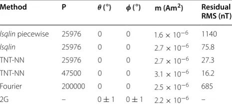
Results are shown in Fig. 7 and Table 2. In Table 2, we also include results from the Fourier method of Lima et al. (2013) and the measured moment using a 2G. The original SIRM field map was bilinearly interpolated to produce a 500 × 400 field map as input to the Fourier

method which then produced a 500×400 distribution

of magnetic sources with a dipole spacing of 50 µ m as described in (Lima et al. 2013).

For these MM data, TNT-NN offers marked enhance-ments over lsqlin. We find an acceptable match between the numerically obtained magnetic moment of the basalt SIRM using TNT-NN, lsqlin, the Fourier method, and the measured moment using a 2G. The residual RMS values produced by TNT-NN are two orders of magnitude lower than that produced by the piecewise lsqlin solution. This is due to multiple factors. Two partial factors are (1) TNT-NN does not exclude any dipole interactions and (2) the lsqlin routine exhibit a slow convergence rate leading to early termina-tion which produces solutermina-tions with elevated residuals. Relative to lsqlin, TNT-NN primarily improves solu-tion residuals by solving the full spatial domain of the sample to avoid nonphysical artifacts at subdivision

boundaries, ultimately yielding solutions that are more physically representative.

The piecewise inversions of the cropped 13.6 mm × 19.1 mm domain using lsqlin require 52.3 min

to calculate a solution. Because these piecewise inver-sions are independent, they can be solved concurrently, requiring a total inversion time that is approximately the same as the time required to solve a single subdivision. If it is necessary to solve the piecewise inversions serially due to computer systems limits the total execution time is scaled by the number of subdivisions. In this analysis, the serial execution time is approximately 261.3 min.

In contemporary computing systems equipped with sufficient memory, lsqlin can be used to solve the entirety of the 13.6 mm × 19.1 mm spatial domain of the sample

without the need for sample subdivision. Without subdi-visions, the high-residual interfaces in the lsqlin solution are removed. This allows the lsqlin method to produce solution residuals similar to those of the TNT-NN. How-ever, this incurs a significant increase in computation time, from 52.3 min for a single subdivision to 59.2 h for the whole spatial domain. This is an increase over the piecewise computation time by a factor of approximately 70.

Solving the same cropped 13.6 mm × 19.1 mm domain

in its entirety using TNT-NN requires only 40.98  min, which is less than the time required to solve a single sub-division of one fifth of the problem. This is an improve-ment of 20% and 600% over the concurrent and serial

lsqlin execution times, respectively. The residual RMS is also improved by two orders of magnitude. Compared to using lsqlin to solve the full spatial domain, the computa-tion time required by TNT-NN to obtain a solucomputa-tion with nearly equivalent residual RMS is 86.7 times less.

Expanding the spatial problem domain to the full measurement domain (19.0 mm × 25.0 mm) and solving

for dipoles spaced at the sampling resolution (100 µ m spacing) almost doubles the number of active variables, from 25,976 to 47,500. While this improves the residual RMS, the improvement is not as significant as the shift away from using subdivisions for piecewise inversion. For the minor improvement in residual RMS, there is a 1.31 h penalty on total execution time to compute the solution, almost 200% longer. Despite the increase in problem size, there is no need to address the scan in a piecewise manner.

Ferromanganese crust

The ferromanganese crust thin section was collected from the Takuyo–Daigo Seamount (22◦41.04′ N 153◦ 14.63′ E, at a depth of 2239 m below the water surface)

as sample HPD#954-R10. This sample is 19 ×  19  mm,

30–60 µ m in thickness, and has previously been used Fig. 5 Relative execution time performance enhancement provided

for paleomagnetic study by Noguchi et  al. (2017b). The SIRM MM data were obtained using a Scanning SQUID Microscope at the Geologic Survey of Japan, National Institute of Advanced Industrial Science and Technology (Oda et al. 2016). Hysteresis loops were measured with a Princeton Measurement Corporation Alternating Gradi-ent Force Magnetometer at the same laboratory. The first use of this thin section for MM experimentation was by Noguchi et al. (2017a), who also provide additional col-lection, composition, and MM experimental conditions.

We restrict our comparisons to the SIRM measure-ments of this sample (Fig. 8), using lsqlin and TNT-NN. We address three scenarios: (1) using 25% of the 2-dimensional spatial sampling resolution (200  µ m dipole spacing) over the entire 32.1 mm × 30.1 mm

meas-urement domain (the same scenario presented by Nogu-chi et al. (2017b)), (2) using a dipole spacing of 160 µ m, which is approximately half the sensor-to-sample dis-tance (319 µm), over a 23.1  mm ×  24.1  mm cropped

region around the sample, and (3) using a dipole spacing of 160 µ m over the entire 32.1 mm × 30.1 mm

measure-ment domain. Due to the prohibitive performance of the

lsqlin method, we restrict our lsqlin analyses to scenario 2. We use TNT-NN to address all three scenarios.

Results are shown in Fig. 9 and Table 3. In all scenarios, the numerical methods obtain magnetic sources with similar remanence magnetization (the arithmetic mean of these is 4.62 ×10−8  Am2 ). These results are on the same order of magnitude, but slightly less than the meas-ured remanence magnetization for this sample obtained by experimental hysteresis (7.52 ×10−8  Am2 , found by Noguchi et  al. (2017b, Table  S1)). lsqlin produces the highest residual RMS value of all scenarios due to early termination (reaching the maximum number of itera-tions). TNT-NN yields lower residual RMS values that are similar for all three inversion scenarios. For these scenarios, the largest solution residual RMS is caused by decreasing the inverse solution resolution and scan area Fig. 6 At left is a reflected light photo of the Hawaiian basalt thin section. At right is the SIRM B z field map (the positive z-direction is out

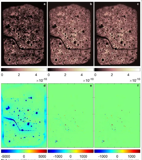
Fig. 7 Comparison of SIRM magnetic sources within the Hawaiian basalt thin section. a The piecewise inverse solution produced using lsqlin using sample subdivision (for a cropped 13.6 mm × 19.1 mm region of the original scan). b The inverse solution produced using TNT-NN for a cropped

13.6 mm × 19.1 mm region of the original scan. The lsqlin solution for the same scenario is visually identical. c The inverse solution produced using

TNT-NN for the full 19.0 mm × 25.0 mm scan region cropped to a 19.1 mm × 13.6 mm view. d Solution residuals for (a). High-magnitude residuals

at subdivision interfaces are evident as blue fringing-fields at the sample boundaries. e Solution residuals for (b). The lsqlin solution residuals for the same scenario are visually identical. f Solution residuals for (c). The field of view of each image is 13.6 mm × 19.1 mm, dipole orientation is out of

page, and units are Am2

(scenario 2). Reducing the field of view so there is less area surrounding the sample causes a small increase in solution residual RMS. It is unlikely that this increase is significant enough to affect interpretation, as can be seen by comparing Fig. 9b, e to 9c, f, respectively.

All numerical solutions appear to increase in blurri-ness from the right to the left across the sample area. The original inversion published by Noguchi et  al. (2017b,

Figure S8) exhibits the same trait. There are multiple fac-tors that could be responsible for this trait, including an irregular sample surface or inconsistent sensor-to-sample distance. Because the original sample varied in thickness from 30–60 µ m, it is possible that the sample surface was not coplanar with the surface of the SSM sensor path. This would result in an inconsistent sensor-to-sample distance and ultimately an inconsistent spatial resolution.

For conventional NNLS methods, scenarios 1 and 2 are solvable, albeit on a scale comparable to problems that required computation times of “several weeks” (Weiss et  al. 2007a) or several days in these analyses [see the Hawaiian basalt inversion in Weiss et al. (2007b)]. Alter-native methods could reduce computation time at the cost of solution residuals (like those in the piecewise lsq-lin basalt solution shown in Fig. 7d). Here, lsqlin required 5.26 times more computation time than TNT-NN to solve scenario 2. For TNT-NN, solving scenarios 1, 2, and 3 required 0.94, 1.18, and 7.89 h, respectively. This is slightly more than 10 h of cumulative computation time.

Speleothem

Speleothems have shown to be excellent natural record-ers of magnetic signals (Latham et  al. 1979; Morinaga et  al. 1985, 1989; Osete et  al. 2012; Strauss et  al. 2013; Font et  al. 2014; Bourne et  al. 2015; Lascu et  al. 2016; Jaqueto et al. 2016; Ponte et al. 2017; Zhu et al. 2017) as they are able to capture and preserve within their calcite matrix, detrital magnetic minerals from airborne par-ticles, drip water or stream water from flood events as well as in situ iron oxy-hydroxide precipitates (Lascu and Feinberg 2011; Denniston and Luetscher 2017).

The stalagmite analyzed here, SVC982, originates from Spring Valley Caverns (SVC) in Fillmore County, Minne-sota, USA, in the Root River watershed of the Upper Mis-sissippi Valley. Additional field site and sample collection details are provided by Dasgupta et al. (2010). A 100 µ m thin section from the top ∼ 5 cm of the speleothem was prepared for SQUID microscopy using non-magnetic equipment and binding materials. In order to obtain a unidirectional field map suitable for inversion, the sample was magnetized using a 1 T field oriented perpendicular to the thin section plane, which resulted in the specimen acquiring a SIRM.

The MM data were collected using the scanning SQUID microscope at the MIT Paleomagnetism Labora-tory. SQUID microscope measurements were performed inside a magnetically shielded environment (ambient field < 100 nT), using a high-precision scanning stage, which allowed data collection along a square grid with 100 µ m spacing. The sensor-to-sample distance was 200 µ m. Typical scan times for a ∼ 10 cm2 area were 16.5 h. The bulk moment of the sample was also measured using a Table 2 Summary of  the  unidirectional basalt inversion

parameters and results

The first column shows the method used to obtain results: the numerical method or a 2G Enterprises Superconducting Rock Magnetometer (2G, shown in the final row). The second column, P, is the number of sample points collected by the scanning SQUID microscope. We set the number of dipoles, equal to the number of samples for each inversion. The third and fourth columns give the unidirectional orientation of the dipoles as used for NNLS analysis. The fifth column lists the moment, m. The final column provides the residual RMS of the NNLS fits with the B z field. 2G data were obtained from Weiss et al. (2007b)

Method P θ ( ◦_{) φ (} ◦_{) m (Am2)} Residual

Fig. 9 Comparison of SIRM magnetic sources within the ferromanganese crust thin section. All inversions were performed using TNT-NN. a The SIRM magnetic moments found using a dipole spacing of 200 µ m, and cropped to a 23.1 mm × 24.1 mm field of view, b the SIRM magnetic

moments found using a 23.1 mm × 24.1 mm cropped view and a magnetic source resolution of half the sensor-to-sample distance (160 µ m dipole spacing), c the SIRM magnetic moments found using the full 30.1 mm × 32.1 mm view and a magnetic source resolution of half the

sensor-to-sample distance (160 µ m dipole spacing) shown using the same 23.1 mm × 24.1 mm field of view as a and b, d solution residuals of a, e

solution residuals of b, and f solution residuals of c. Dipole orientations are out of page and units are Am2

for a–c and nT for d–f

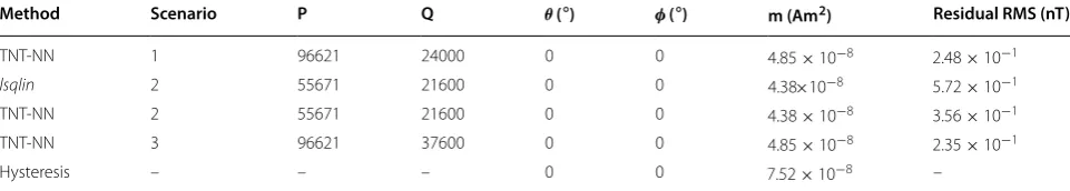
Table 3 Summary of the unidirectional ferromanganese crust inversion parameters and results

The first column shows the method used to obtain results: the numerical method or hysteresis (shown in the final row). The second column shows the scenario with which the parameters and results are associated. The third column, P, is the number of sample points collected by the scanning SQUID microscope. The fourth column, Q, is the number of dipoles in the solution of each inversion. The fifth and sixth columns give the unidirectional orientation of the dipoles as used for NNLS analysis. The seventh column lists the moment, m. The final column provides the residual RMS of the NNLS fits with the B z field. Hysteresis data were obtained from Noguchi et al. (2017b, Table S1)

Method Scenario P Q θ ( ◦) _φ ( ◦) _{m (Am}2₎ Residual RMS (nT)

TNT-NN 1 96621 24000 0 0 4.85

×10−

8 _2.48

×10−

1

lsqlin 2 55671 21600 0 0 4.38×10−

8 _5.72

×10−

1

TNT-NN 2 55671 21600 0 0 4.38_×10−8 3.56_×10−1

TNT-NN 3 96621 37600 0 0 4.85_×10−8 2.35_×10−1

2G Enterprises Rock Magnetometer at the Institute for Rock Magnetism in the Department of Earth Sciences at the University of Minnesota.

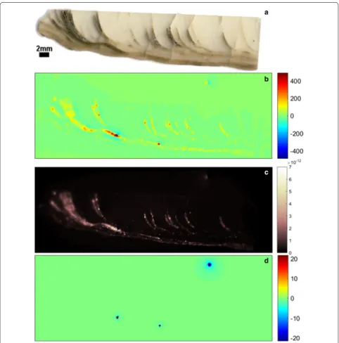
The magnetic minerals within this speleothem are rela-tively sparse due to depositional layering, seen in Fig. 10. Although this sparse spatial distribution of magnetic

material gives rise to a similarly sparse inverse solution, the problem itself is still dense because the Jacobian matrix is dense.

Results are shown in Table 4 and Fig. 10. We find an acceptable match between the numerically obtained magnetic moment of the speleothem SIRM using

Fig. 10 Inversion results for the SVC982 speleothem: a an image of the SVC982 speleothem, b the SIRM B z field map (the positive direction is out of page) obtained by scanning SQUID in nT with the color range scaled to show all the flood layers (the maximum intensity is 3256.4 nT), c the SIRM magnetic moments found using the TNT-NN unidirectional inversion (dipoles out of page) in Am2

TNT-NN, the Fourier method, and the measured moment using a 2G. Due to sample dimensions and instrument configuration, it was necessary to magnetize the sample in the orientation of speleothem growth. The bulk measured moment could be smaller due to the elon-gated nature of the sample, which is not optimal for the 2G coil configuration, which is designed for equidimen-sional samples. The moment could also be affected by the differing numerical and experimental orientations, due to possible magnetic anisotropy of the sample. Two addi-tional numerical reasons contribute to the moment of the TNT-NN solution being higher than the moment of the Fourier solution: (1) the nonphysical sources introduced by TNT-NN inflate the net magnetic moment, and (2) the Fourier solution has variables that do not conform to the non-negativity constraint which deflate the net mag-netic moment of the solution. However, we are not trying to perfectly match the experimental results. Instead, the purpose of this comparison is to determine whether the numerical results are physically reasonable.

The solution residual RMS for this inversion is the same order of magnitude as the residual RMS values for the ferromanganese crust inversions and two orders of magnitude lower than the TNT-NN residual RMS val-ues for the basalt inversions. The residual RMS produced using TNT-NN is lower than that of the Fourier solution; however, both are the same order of magnitude.

One source of high-magnitude residuals in the speleo-them inverse solution can be traced to contamination of the MM scanning environment, outside the sample area (Fig. 10). Removing the magnetic sources and residuals that are not associated with the sample is easily done in postprocessing. Accounting for the interactions of the sample dipoles with the contamination dipoles remains non-trivial. Removing the solution residuals in the spatial vicinity of the contamination only reduces overall resid-ual RMS by 0.169 nT to 0.599 nT.

The remaining sources of high-magnitude residuals are magnetic sources that are high-magnitude relative to the remainder of the sample. This difference in mag-netic source magnitude is significant enough to appear as a sharp discontinuity. Such interfaces are a major source

of residuals for methods that minimize the L2-norm,

like NNLS, as those methods will naturally smooth such interfaces.

This is the largest spatial inversion solved to date, by a factor of 2.26 (the ferromanganese crust scenario 2 pre-sented here is the second largest). Despite the scale of this problem, TNT-NN required just over 24 h of compu-tation time to produce a solution.

Discussion

To achieve reasonable computation times, prior approaches to solving the unidirectional MM inverse problem used lsqlin in lieu of LH-NNLS and to incorpo-rate techniques to reduce computational difficulty (sam-ple subdivision, dipole thresholding, reducing resolution, etc.). TNT-NN provides a transformative method for accelerating the computation of the full spatial unidirec-tional MM inverse problems, without the need to modify the problem in a manner that reduces resolution or the physicality of the solution. For all samples, synthetic and natural, the TNT-NN method consistently offers per-formance enhancement over alternative methods via reduced execution time and solution residual, as seen in Fig. 11.

TNT-NN always requires less time to produce a solu-tion than the other methods tested. For the synthetic UMN logo problem, TNT-NN and LH-NNLS produced identical solutions but TNT-NN was 623 times faster, on average. Using lsqlin to solve the piecewise Hawai-ian basalt inversion problem yields the closest execution time to TNT-NN. The execution time required of lsq-lin to solve the Hawaiian basalt inversion problem in its entirety increases to 59.2 h when solving it in its entirety, 86.7 times slower than TNT-NN.

The computation time spent by TNT-NN to obtain solutions for the ten inversion scenarios presented here totals 1.54 days. Approximately 87% of the total com-putation time was spent on two of the largest problems, requiring 24.36 and 7.89  h, respectively. The remaining problems were all solved in under 1.5 h each.

Table 4 Summary of the unidirectional speleothem inversion parameters and results

The first column shows the method used to obtain results: the numerical method or a 2G Enterprises Superconducting Rock Magnetometer (2G, shown in final row). The second column, P, is the number of sample points collected by the scanning SQUID microscope. The third column shows that we set the number of dipoles, Q, equal to the number of samples for this inversion. The fourth and fifth columns give the unidirectional orientation of the dipoles as used for NNLS analysis. The sixth column lists the moment, m. The final column provides the residual RMS of the NNLS fits with the B z field

The trivial synthetic UMN logo inversion problem is the only case where a competing method matches the residual RMS produced by the TNT-NN solution. For the more computationally intense natural samples, only the small inversions of the Hawaiian basalt and ferromanga-nese crust were attempted using an alternative method. Other scenarios were considered large enough to be intractable and computational tactics violating physical-ity (piecewise inversion and dipole thresholding) were undesirable.

Relative to the piecewise lsqlin Hawaiian basalt solu-tion, the residual RMS of other solutions are two orders of magnitude lower. When using lsqlin to solve the entire spatial domain of the Hawaiian basalt and fer-romanganese crust samples, the residual RMS is the same order of magnitude as that of TNT-NN. However, this incurs additional computation time relative to the TNT-NN method. The TNT-NN algorithm exhibits a minor increase in residual RMS for tested scenarios that increase the spatial domain (field of view) around the sample or reduce resolution. The characteristics of the residual RMS produced by TNT-NN can be attributed to the design of the TNT-NN algorithm.

The core least-squares solver used in TNT-NN (simply named TNT) will, under perfect circumstances, solve the preconditioned system of equations in a single iteration. Because computers cannot yet avoid numerical rounding errors, it is more common that TNT will iterate as long as the residual is decreasing. The computational cost of these iterations is relatively low compared to calculating the TNT preconditioner. As such, early termination has not been found to be necessary in practice (Myre et al. 2018).

Different types of regularization are introduced by the TNT-NN method and by Fourier method of Lima et al. (2013). Whereas both methods assume a fixed direction for the magnetization as a general regularization strat-egy, the TNT-NN method selects a solution by imposing strict non-negativity on the solution and stopping after a convergence criterion is met (no improvement in solu-tion residual); similarly, Wiener deconvolusolu-tion and win-dowing/filtering further regularize the inverse problem in the Fourier domain. Which regularization scheme per-forms best depends on the specific data being inverted and whether the underlying assumptions of each scheme (e.g., non-negativity and smoothness of the solution) are expected based on additional information about the sam-ple. In particular, the overall smoothness of the solution should be carefully analyzed as downward continuation of the magnetic data from the measurement plane to the sample plane is intrinsic to this type of inverse problem. Thus, one should determine the amount of regulariza-tion needed by assessing whether fine-scale changes and peaking in the solution are real or stem from noise mag-nification at higher spatial frequencies. When available, additional information on the magnetization, such as net moment measurements, can further guide the choice of regularization parameter(s).

The TNT-NN method is able to produce solutions to all of the samples using the full spatial domain with-out the need to avoid any computational roadblocks. However, undesirable effects appear in the solutions. Without incorporating any regularization techniques, least-squares methods, and any method minimizing the L2-norm, will produce smooth solutions. The

signals can be lost. In this sense, least-squares methods act like low-pass filters. This low-pass filtering effect is highly likely to occur at the edge of sample, where sharp discontinuities are present. The effect manifests as a nonphysical “halo” in the spatial solution that begins near discontinuities and diminishes in magnitude with sampling distance from the sample. These nonphysical sources can artificially elevate the net moment of the solution. Without additional constraints or regulariza-tion this effect will persist.

The haloing effect is most apparent in the low-resolu-tion synthetic UMN logo spatial solulow-resolu-tions. The smooth transition of the halo region is evident in Fig. 12, where a transect of the TNT-NN and known solutions, and the difference thereof, for scenario 3 of the synthetic UMN logo are shown. The spatial basalt and ferroman-ganese crust solutions also exhibit haloing but it is not immediately apparent. Haloing is not obvious in the spatial solution for the SVC982 speleothem sample, but it is present in low intensities along the depositional bands.

Fourier techniques (Lima et al. 2013; Baratchart et al. 2013) produce high-quality solutions faster than spatial domain techniques. However, an issue similar to halo-ing exists in Fourier solutions. This issue is nonphysical artifacts that manifest as over- and undershoot at sharp interfaces (Hewitt and Hewitt 1979). This was originally discovered by Wilbraham in 1848 but has since come to be known as Gibb’s phenomenon (Gottlieb and Shu 1997). In the context of unidirectional MM inverse prob-lem, undershoot would qualify as a non-negativity con-straint violation.

When comparing TNT-NN and Fourier solutions for the Hawaiian basalt sample (Fig. 13), it is seen that under-shoot violating non-negativity occurs at sample bounda-ries. More accurately, undershoot occurs at strong gradients in the solution (a strong difference in adjacent magnetic moments). This can be seen when comparing the TNT-NN and Fourier solutions for the speleothem sample (Fig. 14). For this sample, undershoot does not occur at sample boundaries, instead it is localized to iso-lated strongly magnetic grains. Despite the presence of undershoot, the Fourier method produces high-quality solutions. These solutions could potentially be exploited as a “starting point” to reduce computation time for spa-tial domain inversion using TNT-NN.

Nonphysical “halos” introduce correspondingly non-physical magnetic sources in the solution. Despite many of these sources being relatively low magnitude, together they affect the bulk moment of the solution. This can be seen in all least-squares results presented here as bulk moment typically increases with the number of dipoles. As more solution dipoles are available, more dipoles can be artificially “inflated” in the nonphysical halo. Fourier solutions obtained using postwindowing can also have low magnitude, nonphysical magnetic sources intro-duced to the solution. Postwindowing acts as a low-pass filter acting to smooth the solution at sharp discontinui-ties by spreading the solution in space.

Ultimately, TNT-NN is capable of solving the full unidirectional MM inverse problem on timescales that are less than or equal to the time required to perform the data acquisition scan using an MM. This provides a means to effectively steer experimentation.