An adjoint data assimilation method for optimizing frictional parameters
on the afterslip area
Masayuki Kano1, Shin’ichi Miyazaki1, Kosuke Ito2, and Kazuro Hirahara1
1Department of Geophysics, Division of Earth and Planetary Science, Faculty of Science, Kyoto University, Kyoto, Japan 2Japan Agency for Marine-Earth Science and Technology, Yokohama, Japan
(Received March 13, 2013; Revised August 7, 2013; Accepted August 7, 2013; Online published December 6, 2013)
Afterslip sometimes triggers subsequent earthquakes within a timescale of days to several years. Thus, it may be possible to predict the occurrence of such a triggered earthquake by simulating the spatio-temporal evolution of afterslip with estimated frictional parameters. To demonstrate the feasibility of this idea, we consider a plate interface model where afterslip propagates between two asperities following a rate-and-state friction law, and we adopt an adjoint data assimilation method to optimize frictional parameters. Synthetic observation data are sampled as the slip velocities on the plate interface during 20 days. It is found that: (1) all frictional parameters are optimized if the data sets consists not only of the early phase of afterslip or acceleration, but also of the decaying phase or deceleration; and (2) the prediction of the timing of the triggered earthquake is improved by using adjusted frictional parameters.
Key words:Afterslip, frictional parameters, data assimilation, earthquake cycle simulation, adjoint method.
1.
Introduction
The prediction of the occurrence time of earthquakes, based on physics-based models, is a highly challenging goal of earthquake science (e.g., Kato, 2008). Difficulties are rooted in the following facts: (1) the governing equations may not be sufficiently accurate to forecast the temporal evolution of the stress and the slip velocity; (2) it gener-ally takes several hundred years to obtain observations over multiple cycles; and (3) differential equations are so stiff, and therefore the period when we might observe any pre-cursory signals would be quite limited, so that, to date, un-ambiguous precursory signals have never been observed.
Nevertheless, this does not mean that all earthquakes are entirely unpredictable. An earthquake leads to a stress in-crease around the rupture region, which may either trigger another earthquake or induce afterslips. Continuous GPS measurements have revealed that afterslip lasts for several years following giant (M8–9) earthquakes (e.g., Heki et al., 1997). Such afterslip would load another asperity (a strongly-coupled area on the fault), if it exists, and con-sequently another earthquake would be induced there, de-pending on the stress state on the asperity, the amplitude of perturbation and the relative distance between asperities. For example, Uchidaet al.(2009) suggested that afterslip east of the 2003 Tokachi-oki earthquake rupture region had propagated eastward and triggered the 2004 Kushiro-oki earthquake. Thus, if we trace the spatio-temporal evolution of afterslip, it may be possible to predict the occurrence of such a triggered earthquake.
Copyright cThe Society of Geomagnetism and Earth, Planetary and Space Sci-ences (SGEPSS); The Seismological Society of Japan; The Volcanological Society of Japan; The Geodetic Society of Japan; The Japanese Society for Planetary Sci-ences; TERRAPUB.
doi:10.5047/eps.2013.08.002
In order to predict the occurrence time of a subsequent earthquake, it is essential to know the reasonable frictional property on the fault and to develop accurate physical mod-els. Frictional properties in afterslip areas have been esti-mated based on kinematic inversions of GPS data (Miyazaki
et al., 2004; Hsu et al., 2006) or dynamic model-based simulations, which provide constraints on the evolution of slip and the stress state (e.g., Maroneet al., 1991; Hearn
et al., 2002; Mont´esi, 2004; Perfettini and Avouac, 2004, 2007; Perfettiniet al., 2005; Johnsonet al., 2006; Fukuda
et al., 2009; Mitsuiet al., 2010). It should be noted that all of these studies have employed a rate- and state-dependent friction law (e.g. Dieterich, 1979; Ruina, 1983). Although kinematic inversion is a simple technique, it is limited to estimating only (a −b)σeff, where a and b are
constitu-tive frictional parameters (Eq. (1)) andσeff is the effective
normal stress. Fukudaet al. (2009) developed a Markov chain Monte Carlo (MCMC)-based method (e.g., Metropo-liset al., 1953). Their study represented the Kurile Trench with a one-degree-of-freedom spring-slider system, and es-timated(a−b)σeff,aσeffandL(Lis the characteristic length
(Eqs. (1)–(2)). Mitsuiet al.(2010) applied a Sequential Im-portance Sampling (SIS) method (e.g., Liuet al., 2000) to a two-degrees-of-freedom cell model and demonstrated with synthetic afterslip data that the method worked for estimat-inga−bandL. These previous studies are notable because the probability density functions (PDFs) are successfully re-produced given a numerical model with 106ensemble
mem-bers (Fukudaet al., 2009). However, if we recall that earth-quake simulations with a continuum medium require signif-icant computational resources, (e.g., a single calculation by Ohtaniet al. (submitted toGeophysical Research Letters, 2013) required approximately 107s of CPU time), the real-ization of 106 ensemble members is not practical. Thus, a
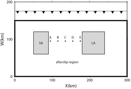
Fig. 1. Plate model domain used in this study. The thick rectangle is the fault area. The two shaded regions represent a large (LA) and small (SA) asperity, respectively. The region around the asperities is assumed to accommodate afterslip. The plate is subducting at a dip angle of 20◦. The solid triangles with thin lines schematically show the trench.
computationally-efficient method is required for estimating frictional parameters which enables a realistic model.
Kanoet al.(2010) utilized an efficient dynamic model-based method, “An Adjoint Data Assimilation Method” (e.g., Lewis and Derber, 1985). Adjoint methods have been extensively applied to realistic models with 106–1010 vari-ables in the fields of meteorology and oceanography for real-time and long-term forecasting. Kanoet al.(2010) first applied an adjoint method to earthquake simulations with a three-degrees-of-freedom cell fault model and estimated
a−b,aandL. They confirmed that the method is compu-tationally much more efficient than MCMC and SIS, whilst providing nearly identical results. They also found thata−b
is always constrained. However, the initial phase data of decaying afterslip is required to constrainL, andawas not constrained under any conditions.
Although Kanoet al.(2010) estimated frictional param-eters for three cell faults, they did not investigate the po-tential impact on earthquake prediction. Nevertheless, their work has motivated us to test the feasibility of predicting future afterslip propagation and its triggering of another earthquake with a realistic continuum fault model based on an adjoint method. In this work, we perform a synthetic data assimilation experiment with the fault model. A rate-and state-dependent friction law rate-and the slowness law (Di-eterich, 1979) are used as governing equations for data as-similation. Although this fault model is still simplified in many aspects, it constitutes an important step toward pre-dicting an actual triggered earthquake by evaluating the po-tential impact of efficient data assimilation.
In Section 2, the numerical model, synthetic afterslip data and the data assimilation system are described. Numerical results are given in Section 3. Section 4 provides a summary and discusses potential challenges for practical application.
2.
Setting
2.1 Forward model
2.1.1 Fault model and frictional properties The model region of the plate boundary at the Kurile Trench is
represented as one rectangular fault (300-km long, 150-km wide) with a dip angle of 20◦(Fig. 1). The model region in-volves two asperities, one large (60-km long, 60-km wide, hereafter LA) and one small (40-km long, 60-km wide, hereafter SA), representing asperities for the Tokachi-oki earthquake and the Kushiro-oki earthquake, respectively. The remainder of the region, subdivided into 10×10-km subfaults, is the aseismic slip region where afterslip is ex-pected to occur.
2.1.2 Governing equations The governing equations consist of a rate- and state-dependent friction law (Eq. (1)), a slowness law (Eq. (2)), and the time derivative of a quasi-dynamic equation of motion (Eq. (3)) as shown below:
μiσi =μ0iσi+aiσiln
Vi V0i
+biσiln
V0iθi Li
, (1)
dθi dt =1−
Viθi
Li , (2)
σi dμi
dt =
j
ki jVpl−Vj
− G
2c d Vi
dt , (3)
whereμi is a frictional coefficient, Vi is the slip velocity, θi is a state variable,σiis the effective normal stress,V0i is
a reference velocity,μ0iis a reference frictional coefficient
whenVi =V0i at steady state, andai,bi, Li are frictional
parameters (hereafter, we useAi =aiσi,Bi =biσi) at cell i. In addition,Vplis the plate velocity,Gis the shear
mod-ulus, andcis the shear wave velocity. The slip response functionki jrepresents shear stress changes at celli due to the unit slip at cell j, and is calculated by Okada (1992). The second term on the right-hand side of Eq. (3) is a radia-tion damping term that represents energy loss by shear wave radiation (Rice, 1993). This set of equations is solved for
μi,Vi andθi. We setVpl =9 cm/yr (DeMetset al., 1994),
G =30 GPa,c=3 km/s,μ0i =0.6, andV0i =Vpl(=9
cm/yr). We set the effective normal stressσi =100 MPa in
the asperity region andσi =20 MPa in the afterslip region,
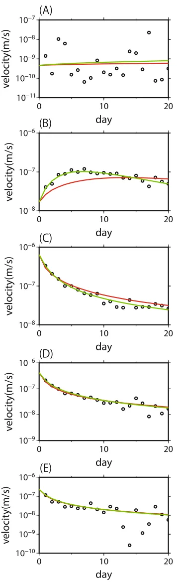
Fig. 2. Time series of slip velocity at points A–E in Fig. 1 with those cal-culated with first-guess and estimated values. Circles show the synthetic observation data. Red and green lines show the calculated slip velocity with first-guess and estimated values in Table 1, respectively.
We first calculate the spatio-temporal evolution of afterslip with the frictional parameters (A−B,A,L) estimated from the subdaily GPS time series following the 2003 Tokachi-oki earthquake by Fukudaet al.(2009). However, afterslip does not propagate more than 40 km in the strike region
us-ing their values of (A−B(kPa),A(kPa),L(mm))=(218, 300, 1.00). This is because the single spring-slider system used in their work is not realistic. We found that a low ef-fective normal stress with high pore pressure is essential for afterslip to propagate at a similar depth to seismogenic zones (e.g., Ariyoshiet al., 2007). Equations (1) to (3) are numerically solved with an adaptive time-step Runge-Kutta method (Presset al., 1996) under the initial conditions of
Vi =0.9Vplandθi =Li/Vi.
2.1.3 True state We adopt a one model realization with frictional parameters ((A−B(kPa),A(kPa),L(mm))
=(−100, 40.0, 40.0) in LA, (−80.0, 40.0, 40.0) in SA, and (5.00, 40.0, 40.0) in the afterslip regions, as a ‘true’ state. This is obtained from forward time integration of the above governing equations.
The true state indicates that large earthquakes occur quasi-periodically in the LA region at approximately 100-year intervals, and medium-sized earthquakes occur in the SA region with an average interval of 60 years, depend-ing on the stress interactions between the two asperities (throughout this paper, we regard a fault slip as an earth-quake when the slip velocity exceeds 1 cm/s). This is a typical timescale for thrust-type earthquakes at the Kurile Trench (e.g., Sawaiet al., 2009).
Hereafter, we focus on one particular earthquake in the LA region which occurred 894 years after the initial time. The subsequent afterslip triggered an earthquake at SA 3.83 years after the first earthquake. Hereafter, the timeframe refers to one day after the initiation of the first earthquake. Figure 2 shows the time series of the slip velocity due to afterslip, showing that the accelerating phase is found at point B. The triggered earthquake occurred at t = 3.83 years.
2.2 Synthetic data and simulation run
We investigate whether synthetic observations are suffi-cient to specify the frictional parameters over the afterslip region. Synthetic slip velocity observation on the fault is sampled from the true state during days 1–20 at all cells in the afterslip area. We then added a Gaussian error with zero mean and standard deviation 1.0×10⁻⁸m/s (Miyazaki
et al., 2004). We assimilate these synthetic slip velocity data through the adjoint data assimilation method to check whether the “first-guess” parameter values are updated to their true values.
In actual cases, accurate frictional parameters are rarely known. However, it may be reasonable to provide a first-guess value within the order of parameters that is predeter-mined by, for example, kinematic inversions. In this study, we perform a time integration with the first-guess frictional parameter values in the afterslip region (hereafter, simula-tion run). In this work, we perturb the true fricsimula-tional param-eters by 100% to generate the first-guess values, as shown in Table 1. Note that the frictional parameters in the two as-perities and the initial values of shear stress and slip velocity are fixed to their true values throughout the experiment.
2.3 Adjoint data assimilation method
The adjoint-based data assimilation is outlined in this section. More detailed explanations are given in Lewiset al.
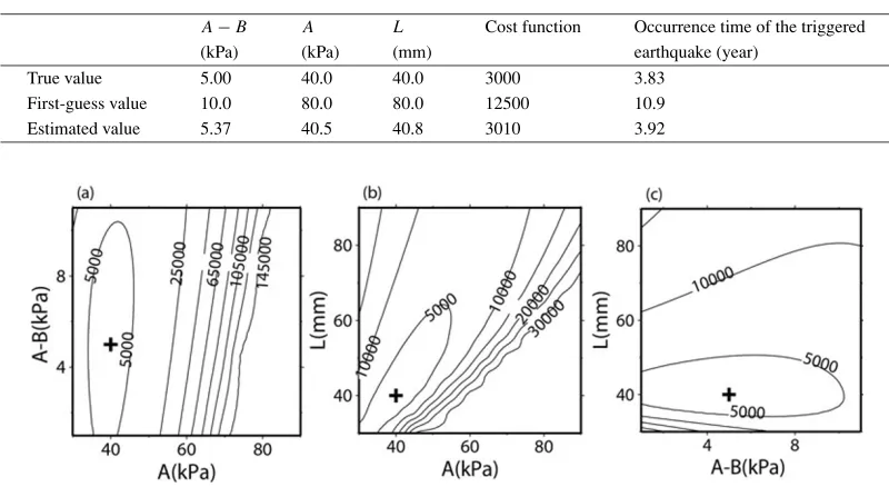
Table 1. Table of true, first-guess and estimated values of frictional parameters, cost function, and occurrence time of the triggered earthquake.
A−B A L Cost function Occurrence time of the triggered
(kPa) (kPa) (mm) earthquake (year)
True value 5.00 40.0 40.0 3000 3.83
First-guess value 10.0 80.0 80.0 12500 10.9
Estimated value 5.37 40.5 40.8 3010 3.92
Fig. 3. Contour maps of cost function: (a)A:A−B, (b)A:L, and (c)A−B:Lplanes. The crosses show the true values.
results and the observations. The adjoint model, which is the adjoint of the dynamic model operator linearized about the time trajectory, effectively transforms the misfit into the gradient of the cost function with respect to control vari-ables, i.e. the frictional parameters in this study. The con-trol variables are updated iteratively in order to minimize the cost function, thereby improving estimates and predic-tion. Note that, in each iteration, the control variables are constant.
The cost function used in this work is defined as follows:
J(C)= 1
2
t
(Vsimt (C)−Vobst )TRt−1(Vsimt (C)−Vobst ), (4)
whereRt is an observation error variance-covariance
ma-trix,Cis a vector that consists of frictional parameters, i.e.,
C=[A−B,A,L]T,Vsimt represents a simulated slip
veloc-ity vector at epochtandVobst is a corresponding observation
vector.
We first perform forward time integration with the first-guess values and then an adjoint model transforms the misfit into the gradient of the cost function with respect to the control variables,∂J/∂C. In this work, the control variables are updated as follows:
Cnew=Cold+αC ∂J ∂C
C=Cold
, (5)
whereαCis a constant and is different in each parameter,
i.e.,
αA−B = −2.5
∂J ∂(A−B)
iter=1
, (6)
αA = −20
∂J ∂A
iter=1
, (7)
αL = −20
∂J ∂L
iter=1
, (8)
We then iterate this calculation either 30 times, or until the updated cost function satisfies the following criteria:
Jold−Jnew
Jnew <
0.001 (9)
If Jnew becomes greater than Jold, we change the constant αCtoαC/2 untilJnewbecomes smaller thanJold. Note that
alpha values do not affect the estimation and convergence rate, and that this convergence condition (Eq. (9)) is suffi-cient to obtain a robust result.
3.
Results
3.1 Optimization of frictional parameters
Table 1 shows the results of data assimilation, “estimated values” and first-guess values. As a result of data assimi-lation, frictional parameters are updated to (A−B (kPa),
A(kPa),L (mm))=(5.37, 40.5, 40.8), which are close to the true parameters, (5.00, 40.0, 40.0). Figure 2 shows that the updated state of the slip velocity is consistent with the observed values at points A–E, whereas those in the simula-tion run were not. We confirmed, by follow-up experiments, that this result is true within the range of first-guess values which are one-order larger, or smaller, than the true values. This suggests that the rough estimate of first-guess values is sufficient to recover the true frictional parameters. The rea-son why all frictional parameters are determined, unlike in Kanoet al.(2010), is presumably that the observation data are available during the accelerating phase of the afterslip. Moreover, we found that only the observations at point B constrain all frictional parameters. Thus, we suggest that if there is at least one observation which contains both the acceleration phase and the decaying phase, all frictional pa-rameters are constrained.
Fig. 4. Updates of the frictional parameters: (a)A: A−B, (b)A :L, and (c)A−B: Lplanes. The arrows indicate the updates of the frictional parameters from the first-guess to the estimated values. Circles also indicate the values at each iteration and the number of iterations. Stars indicate the true values.
Fig. 5. Snapshots of the slip velocity at (a)t=3.50 yr and (b)t=4.00 yr, respectively. In each figure, the slip velocity is calculated with (1) true, (2) first-guess and (3) estimated values, respectively.
the robustness of the solution. Figure 4 shows three param-eter values at each iteration. Paramparam-eter values converged only after 24 iterations. The computational cost of each iteration of this data assimilation system is approximately twice that of the forward calculation, and is therefore about 50 times greater in total. This demonstrates the efficiency of an adjoint data assimilation method compared with Monte Carlo-based methods or the explicit illustration of the cost function by iteratively changing frictional parameters as in Fig. 3.
3.2 Prediction of the triggered earthquake in SA
The occurrence time of the triggered earthquake with estimated parameters ist = 3.92 year (Table 1). This is close to the true state,t = 3.83 year, compared with t =
10.9 year without optimization. Figure 5 shows snapshots of the slip velocity at (a) t = 3.50 yr and (b) t = 4.00 yr, calculated with (1) true values, (2) first-guess values, and (3) estimated values, respectively. This figure shows the weakening of the locked interface at SA and afterslip before, and after, the triggered earthquake in the true state
with true values and estimated values, respectively, but not with first-guess values. These results indicate that only the observations during 20 days contribute to improvements in the prediction of the triggered earthquake. Although this data assimilation is an idealized experiment, it encourages us to develop a prediction system for triggered earthquakes with actual data and a more sophisticated fault system.
4.
Discussion and Summary
are constrained.
In terms of a practical application, several points need to be further verified. First, predictions derived from a data assimilation system are strongly dependent on the base dy-namic model. Currently, the dydy-namic model does not con-sider the geometry of the plate boundary, structural het-erogeneity and visco-elasticity. We assumed uniform fric-tional parameters over the entire afterslip region. Moreover, it would be essential to estimate the frictional parameters in asperity (Hiyoshiet al., Possible estimates of frictional properties on earthquake and afterslip rupture surfaces with 4D-VAR method, manuscript in preparation, 2013) and other control variables, i.e. the initial slip velocity and the initial state variable (Kanoet al., 2010). Our future scope includes improvement of the base model, especially the model of friction, to explain the data well and the optimiza-tion of heterogeneous parameters.
Acknowledgments. We thank T. Ochi for useful comments that helped to improve the manuscript. This work was supported by JSPS Fellows (23-1546), by MEXT KAKENHI (21340127) and by MEXT projects of “New Research Project for the Evaluation of Seismic Linkage around the Nankai Trough” and of “Observation and Research Program for Prediction of Earthquakes and Volcanic Eruptions”. We used Generic Mapping Tools (Wessel and Smith, 1998) to produce the figures.
References
Ariyoshi, K., T. Matsuzawa, and A. Hasegawa, The key frictional parame-ters controlling spatial variations in the speed of postseismic-slip prop-agation on a subduction plate boundary,Earth Planet. Sci. Lett.,256, 136–146, 2007.
DeMets, C., R. G. Gordon, D. F. Argus, and S. Stein, Effect of recent revisions to the geomagnetic reversal time scale on estimates of current plate motions,Geophys. Res. Lett.,21, 2191–2194, 1994.
Dieterich, J. H., Modeling of rock friction 1. Experimental results and constitutive equations,J. Geophys. Res.,84, 2161–2168, 1979. Fukuda, J., K. M. Johnson, K. M. Larson, and S. Miyazaki, Fault
fric-tion parameters inferred from the early stages of afterslip follow-ing the 2003 Tokachi-oki earthquake,J. Geophys. Res.,114, B04412, doi:10.1029/2008 JB006166, 2009.
Hearn, E. H., R. B¨urgmann, and R. E. Reilinger, Dynamics of ˙Izmit earthquake postseismic deformation and loading of the D¨uzce earthquake hypocenter, Bull. Seismol. Soc. Am., 92, 172–193, doi:10.1785/0120000832, 2002.
Heki, K., S. Miyazaki, and H. Tsuji, Silent fault slip following an interplate thrust earthquake at the Japan Trench,Nature,386, 595–597, 1997. Hsu, Y.-J., M. Simons, J.-P. Avouac, J. Galetzka, K. Sieh, M. Chlieh, D.
Natawidjaja, L. Prawirodirdjo, and Y. Bock, Frictional afterslip follow-ing the 2005 Nias-Simeulue earthquake, Sumatra,Science,312, 1921– 1926, doi:10.1126/science.1126960, 2006.
Ito, K., Y. Ishikawa, Y. Miyamoto, and T. Awaji, Short-time-scale pro-cesses in a mature hurricane as a response to sea surface fluctuations,J. Atmos. Sci.,68(10), 2250–2272, 2011.
Johnson, K. M., R. B¨urgmann, and K. M. Larson, Frictional properties on the San Andreas fault near Parkfield, California, inferred from models of afterslip following the 2004 earthquake,Bull. Seismol. Soc. Am.,96, S321–S338, doi:10.1785/0120050808, 2006.
Kano, M., S. Miyazaki, K. Ito, and K. Hirahara, Estimation of frictional parameters and initial values of simulation variables using an adjoint data assimilation method with synthetic afterslip data,Zishin 2,63, 57– 69, 2010 (in Japanese).
Kato, N., Numerical simulation of recurrence of asperity rupture in the Sanriku region, northeastern Japan, J. Geophys. Res.,113, B06302, doi:10.1029/2007 JB005515, 2008.
Kitagawa, G., Monte Carlo filter and smoother for non-Gaussian nonlinear state space models,J. Comput. Graph. Stat.,5, 1–25, 1996.
Lewis, J. and J. Derber, The use of adjoint equations to solve a variational adjustment program with advective constraint,Tellus,37A, 309–322, 1985.
Lewis, J., S. Lakshmivarahan, and S. Dhall,Dynamic Data Assimilation: A Least Squares Approach, 654 pp, Cambridge University Press, 2006. Liu, J., R. Chen, and T. Logvinenko, A theoretical framework for
sequen-tial importance sampling and resampling, inSequential Monte Carlo in Practice, 225–242, Springer-Verlag, 2000.
Marone, C. J., C. H. Scholz, and R. Bilham, On the mechanics of earth-quake afterslip,J. Geophys. Res.,96, 8441–8452, 1991.
Metropolis, N., A. W. Rosenbluth, M. N. Rosenbluth, A. H. Teller, and E. Teller, Equation of state calculations by fast computing machines,J. Chem. Phys.,21, 1087–1092, 1953.
Mitsui, N., T. Hori, S. Miyazaki, and K. Nakamura, Constraining inter-polate frictional parameters by using limited terms of synthetic obser-vation data for afterslip: a preliminary test of data assimilation,Theor. Appl. Mech. Jpn.,58, 113–120, 2010.
Miyazaki, S., P. Segall, J. Fukuda, and T. Kato, Space time distribution of afterslip following the 2003 Tokachi-oki earthquake: Implications for variations in fault zone frictional properties,Geophys. Res. Lett.,31, L06623, doi:10.1029/2003 GL019410, 2004.
Mont´esi, L. G. J., Controls of shear zone rheology and tectonic loading on postseismic creep,J. Geophys. Res.,109, B10404, doi:10.1029/2003 JB002925, 2004.
Okada, Y., Internal deformation due to shear and tensile faults in a half-space,Bull. Seismol. Soc. Am.,82, 1018–1040, 1992.
Perfettini, H. and J.-P. Avouac, Postseismic relaxation driven by brittle creep: A possible mechanism to reconcile geodetic measurements and the decay rate of aftershocks, application to the Chi-Chi earthquake, Taiwan,J. Geophys. Res.,109, B02304, doi:10.1029/2003 JB002488, 2004.
Perfettini, H. and J.-P. Avouac, Modeling afterslip and aftershocks fol-lowing the 1992 Landers earthquake,J. Geophys. Res.,112, B07409, doi:10.1029/2006 JB004399, 2007.
Perfettini, H., J.-P. Avouac, and J.-C. Ruegg, Geodetic displacements and aftershocks following the 2001 Mw=8.4 Peru earthquake: Implication for the mechanics of the earthquake cycle along subduction zones,J. Geophys. Res.,110, B09404, doi:10.1029/2004 JB003522, 2005. Press, W. H., S. A. Teukolsky, W. T. Vetterling, and B. P. Flannery,
Numer-ical Recipes in Fortran 77: The Art of Scientific Computing, 2nd edition, 963 pp, Cambridge University Press, New York, 1996.
Rice, J. R., Spatio-temporal complexity of slip on a fault,J. Geophys. Res., 98, 9885–9907, 1993.
Ruina, A., Slip instability and state variable friction laws,J. Geophys. Res., 88, 10359–10370, 1983.
Sawai, Y., T. Kamataki, M. Shishikura, H. Nasu, Y. Okamura, K. Satake, K. H. Thomson, D. Matsumoto, Y. Fujii, J. Komatsubara, and T. T. Aung, Aperiodic recurrence of geologically recorded tsunamis during the past 5500 years in eastern Hokkaido, Japan,J. Geophys. Res.,114, B01319, doi:10.1029/2007JB005503, 2009.
Uchida, N., S. Yui, S. Miura, T. Matsuzawa, A. Hasegawa, Y. Motoya, and M. Kasahara, Quasi-static slip on the plate boundary associated the 2003 M8.0 Tokachi-oki and 2004 M7.1 off-Kushiro earthquakes, Japan, Gondowana Res.,16, 527–533, 2009.
Wessel, P. and W. H. F. Smith, New, improved version of Generic Mapping Tools released,Eos Trans. AGU,79(47), 579, doi:10.1029/98EO00426, 1998.