356 RAUZI AND HANSON
runoff and increase the amount of available precipitation enter- ing the soil for plant use.
beef cows and calf production on mixed prairie vegetation on west- ern South Dakota ranges. South Dak. Agr. Exp. Sta. Bull. 412. 39 p. LITERATURE CITED
DYKSTERHUIS, E. J., AND E. M. SCHMUTZ. 1947. Natural mulches or “litter” of grasslands: with kinds and amounts on a Southern prai- rie. Ecology 28: 163-179.
HERSHFIELD, DAVID M. 1961. Rainfall frequency atlas of the United States. U. S. Dep. Commerce, Weather Bureau Tech. Paper No. 40.
JOHNSTON, ALEXANDER. 1962. Effects of grazing intensity and cover on the water-intake rate of fescue grassland. J. Range Manage. 15: 79- 82.
JOHNSON, LESLIE E., LESLIE R. ALBEE, ALVIN MOXON, AND R. 0. SMITH. 1951. Cows, calves and grass: Effects of grazing intensities on
LEWIS, JAMES K., LESLIE R. ALBEE, G. M. VAN DYNE, AND F. W. WHET- ,.-ZAL. 1956. Intensity of grazing-its
effect on livestock and forage pro- duction. South Dak. Agr. Exp. Sta. Bull. 459. 44 p.
RAUZI, FRANK. 1963. Water intake and plant composition as affected by differential grazing on range- land. J. Soil and Water Cons. 18: - 114-116.
Application and Integration of Multiple Linear
Regression and Linear Programming in
Renewable Resource AnalyseC2
GEORGE M. VAN DYNE3
Ecologist, Radiation Ecology Section, Health Physics Division, Oak Ridge National Laboratory, Oak Ridge, Tennessee, and Associate Professor of Biology, Univer- sity of Tennessee, Knoxville.
HighLight
This paper presents preliminary results of formulating quantitatively the influence of site factors on vari- ous nutrient production measures and using these relationships in linear programming models fo defer- mine the optimum protein produc- tion on a foothill range. Site char- acterisfics for optimum protein pro- duction were constrained to fall within the range of variables mea- sured, and were constrained to safis- fy certain inherent relationships known about these variables. This example shows a useful application of an operations research technique to resource evaluation problems.
1Thi.s research was supported by the
Atomic Energy Commission under
contract with the Union Carbide Corporation. J. S. Olson and B. C. Patten are acknowledged for their suggestions in this research and for review of the manuscript.
2 Paper presented at 19th annual
meeting, American Society of
Range Management, New Orleans,
La., February 1-4, 1966.
3Present address: College of Forestry
and Natural Resources, Colorado
State University, Fort Collins.
Large, fast digital computers have become available in the last 15 years and have allowed the development of special methods of analyzing and studying com- plex systems in industry and government. Range ecosystems are good examples of complex systems, and it is inevitable that mathematical analysis will be- come increasingly important in the future in range research and range management, as well as in many phases of renewable re- source management. To take ad- vantage of the methodological and conceptual advances from operations research and systems analysis means we will have to give increased attention to for- mulating and studying range problems in mathematical terms. This paper reports only an in- troductory approach in applying and integrating multiple linear regression and linear program-
RAUZI, FRANK, AND A. R. KUHLMAN. 1961. Water intake as affected by soil and vegetation on certain western South Dakota rangeland. J. Range Manage. 14:267-271. RHOADES, EDD, L. F. LOCKE, E. H. MC-
ILVAIN, AND H. M. TAYLOR. 1964. Water intake on a sandy range as affected by 20 years of differential cattle stocking rates. J. Range Manage. 17: 185-190.
SHARP, A. L., J. J. BOND, A. R. KUHL- MAN, J. K. LEWIS, AND J. W. NEW- BERGER, 1964. Runoff as affected by intensity of grazing on rangeland. J. Soil and Water Cons. 19: 103-106. WHITE, EVERETT M., AND R. G. BONE-
STALL. 1960. Some gilgaied soils in South Dakota. Soil Sci. Sot. Am. Proc. 24: 305-309.
ming methods in studying what I call the “optimum site prob- lem.” The work at present is neither exhaustive nor complete but will serve to show, with real- istic examples, the potential of these techniques for learning more about range ecosystems.
The purpose of this paper is (i) to show the development of the quantitative formulation of site relationships to vegetation productivity, (ii) to use multiple linear regression equations as ob- jective functions in, and to de- velop constraints for linear pro- gramming models, and (iii) to show by example and discussion where these approaches have ap- plication in analysis of renew- able resource management prob- lems.
The Range Site
OPTIMUM SITE PROBLEM
OVERFLOW cLAYEY
-SILTY
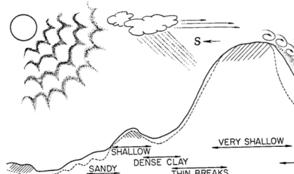
FIG. 1. A diagrammatic representation of the foothill range site complex showing variations in parent materials, soil
factors. Double-ended arrows show discrete.
elude the angle at which sun- light strikes the soil surface and the exposure to the prevailing winds, which may be especially important in drifting snow onto leeward slopes. The ultimate re- sult is the development, over a long period of time, of varying soils and topographic features which, when considered together with precipitation zones, we group arbitrarily into range sites, and to which we can ascribe a characteristic kind and amount of vegetation. The boundaries of range sites usually are not distinct, but they tend to inter- grade and overlap in part. The range site name as such is of value, especially for large-scale surveys, but adds little to our quantitative knowledge about the relationships of the vegeta- tion to the site factors.
Often it is desirable to be able to assess or to rank a given en- vironmental complex such as a range site, a forest area, or some other unit according to some prescribed scheme of practical or theoretical importance. The as- sessment or ranking of a site im- plies that the various properties of this site have a functional re- lationship to criteria which are being ranked. Means of assess- ing the combined effects of site
depths, elevation, exposure, and climatic that boundaries of range sites are not
variables on some criteria have undergone long development originating with qualitative characterizations, and more re- cently turning to quantitative assessments.
Historical Development An early qualitative statement, pertinent to the range site problem and attributed to Darwin, is that a particular plant community is se- lected from the available flora by the environment of a particular lo- cale. This statement illustrates the early recognition that the various environmental factors, acting upon an original flora, lead to the devel- opment of a particular plant com- munity. This notion was developed further by Dokuchaev (1898, referred to by Jenny, 1961), the Russian soil scientist, who formulated the follow- ing relationship.
s = f (Cl, 0, P) (I) where S refers to soils, Cl refers to macroclimate, 0 to organisms (pre- sumably both plants and animals), and P to parent material. Later Jenny (1941) reformulated this re- lationship and added two new inde- pendent variables as follows:
S = f (Cl, 0, R, P, t) (2) where Cl, P, and S are defined as above, R refers to relief, and t to time. Jenny defines 0 as available flora and fauna so that it can be considered an independent variable rather than a dependent variable. This equation states that soil prop-
erties are dependent upon the in- fluences of the climate acting over time on the original conditions of organisms, relief, and parent mate- rial. Similarly, Major (1951) has shown that vegetation is a function of the same state factors or inde- pendent variables. Later Jenny (1961) formulated a more general set of equations for an open system as follows:
1, s, v, or a = f (L,, P,, t) (3) where the dependent variables are any property of the total ecosystem
(l), soils (s), vegetation(v), or animal community (a). The independent variables here are specified by the vector L,, which gives the initial stat: conditions, P, which are the flux potentials, and t again referring to time. In the present sense, flux refers to the movement of matter and energy to and from contiguous ecosystems.
In all of the above formulations the time scale aproximates that of primary succession, evolutionary time, or geologic time. For a short time scale, such as much less than the time required for secondary suc- cession, and for practical purposes, certain of the variables considered dependent variables in the above formulations may be considered to be independent variables. A change in terminology is introduced so that now independent and dependent are used in the conventional statistical sense rather than adhering strictly to Jenny’s (1941) meanings. The sta- tistical usage is denoted by asterisks. Thus, a new relationship may be for- mulated as follows:
V” = f (Cl*, R”, S*) (4) or
Y = f (Xi, X2, . . . X,,, lb,, bz, . . . b,,,)
358 VAN DYNE
are partial regression coefficients. The number of independent vari- ables on any given range site is large, and their measurement be- comes subject to practical consider- ations.
The Regression Model
Y = b,X, + blXl + b2X2 + . . . b,X, The relationship of the vege- tation variable, i.e., yield or com- position, to any given indepen- dent variable may be nonlinear, and certain independent vari- ables may have interacting in- fluences. Development of a “mechanistic” model for predict- ing a vegetation variable, say productivity, no matter how in- teresting a modelling task, is unnecessary for the present pur- poses. As a first approximation and simplification for illustra- tive purposes, an empirical model for predicting a vegeta- tion variable may be obtained by regression analyses. Multiple regression analysis techniques may be used to derive a first order model (linear terms only, without interaction) relating the independent site variables and the dependent vegetation vari- able, giving an equation as follows:
n or Y = I: (brX1)
i=O
(5)
where Y is the dependent vari- able, e.g., yield or composition of the vegetation, X0 is assigned the value one and the other X’s are the independent variables, i.e., independent concerning time fixed to a narrow range. The value of such equations, of course, depends upon the sam- pling scheme in which the data were collected, the inherent variability of the population be- ing sampled, and many other factors whose discussion is be- yond the scope of this paper. Further information on the de- velopment and use of multiple regression models, both linear and nonlinear, may be found in statistical texts such as Ostle
(1963) Hamilton (1964) and Keeping (1962).
The Linear Programming Model The question may be asked,
allXl + aI2 X2 + . . . + aIn, X, 4 cl “How can we select values for the site variables which will maximize the value of the vege- tation property?” The above multiple regression equation for predicting a vegetation variable can be used in a linear program- ming model as an objective func- tion. Then we are interested in learning the values of the X’s which would give us the maxi- mum or minimum value, de- pending on which is desired, of the vegetation variable. If there were no constraints on selecting the values for the X’s and we de- sired to maximize our vegeta- tion variable, one could simply take an extremely large value for each site factor which has a positive partial regression coef- ficient and an extremely small value for those with negative co: efficients. However, in real life this is not possible. Often there is a functional relationship be- tween the variables which can be shown by a set of inequalities as follows:
allX1+a,2X2...a,~X~...al,IX, 4 Ci
(6)
a,,,
X1 $- a,,2 X2 + . . . + anm X,,, 6 cl, where the alj and cl are con- stants. In these inequalities the coefficients ai] may be zero for many of the terms providing that at least one aij is greater than zero. An additional set of constraints in the linear pro- gramming model is that Xi 1 0 for all i. Further background on linear programming models and applications may be found in such texts as Spivey (1963) for introductory treatment and Had- ley (1962) for more advanced treatment. Further considera- tions about constraints pertinent to the optimum site problem follow.Constraints on fhe Solution There are three general types of constraints: (a) inherent rela- tions, (b) those constraints to make the solution realistic, and (c) those imposed to evaluate economical or biological factors. Constraints which are inher- ent in the nature of the inde- pendent variables include the following examples: (i) sand + silt + clay = 100, where me- chanical composition data are expressed in percent; (ii) A hori- zon depth + B horizon depth = depth to C horizon; and (iii) depth to B horizon 4 depth to C horizon. Here, for example, depths of the horizons have func- tional or predictable relation- ships following from their defi- nitions.
Certain constraints are im- posed upon the selection of val- ues for the site factors in order to keep the solution realistic. Thus, for example, the follow- ing conditions represent a first approximation of some boundary conditions for the selection of each site variable in the solution vector:
min. site max.
f;sd
L variablej I in (7) field Constraints may be imposed when certain economical or bio- logical factors are to be con- sidered and which have a func- tional relationship to the de- pendent variable which is being maximized or minimized. In general,
X*am B*mxt S Y” 1x1
(8)
where X”,B”,
and Y” are com- ponents of regression functions for other dependent variables, whose minimum or maximum values are being set according to some heuristic decision about the nature of the solution. An example of such an imposed con- straint follows.equations are developed to pre- dict height of each tree species from the set of site variables. Let the regression equation for spe- cies 1 be used as the objective function in the linear program- ming model. Assume we would like to find the site conditions to maximize height of species 1, yet we want these site conditions to provide at least better than average height for species 2. This can be accomplished by us- ing the regression equation for species 2 as an inequality to be greater than or equal to the mean height of species 2. Four constraints of this type, devel- oped from regression equations for dependent variables other than protein yield, were in- cluded in this problem and are discussed in more detail in the section on the optimum site.
Another realistic considera- tion concerning constraints is that all of the variables in the regression function, i.e., the objective function, are not equally important. Site factors having highly significant rela- tionships with the vegetation parameter could be given addi- tional consideration in the solu- tion, i.e., the solution can be weighted for these variables. A preliminary suggestion on a method to accomplish this would be to use factor or principle com- ponent analyses to get an equa- tion which would be a new linear combination of the more impor- tant independent variables. Such an equation could be used as a constraint to be satisfied in the linear programming solu- tion.
From Dafa fo Models The above equations show how a property of the vegetation may be related quantitatively to mea- surable site factors, and they show how these relationships can be used to formulate an ob- jective function and constraints in a linear programming model. The regression model is based on
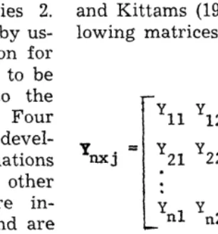
experimental data for the de- pendent vegetation parameters and the independent site factors collected under an appropriate experimental design or sampling plan. To provide a realistic ex- ample, site data and nutrient production data, collected from plots located by multistage ran- domization, are taken from range experiments of Van Dyne and Kittams (1960) and the fol- lowing matrices are defined:
Y =
=d
‘Y
11 y12l ** ‘lj ‘21 ‘22 l *’ '2j
.
.
id y n2 l *’ Y
nj
xNa, = x21X*2 l *. X2j .
. .
x nl xn2...x
n j
!
‘11 ‘12 l ** ‘ljI
(9)
In both Y and X, n = 1,2 . . . 66 plots in one year and 151 plots in another. Each plot or location is considered a site and indepen- dent and dependent variables were measured at each. In Y, j = 1,2, . . . 5 dependent variables: protein yield, grass and sedge composition, perennial grass yield, phosphorus yield, and lig-
nin composition. In X, m = 1,2, . . . 11 topographic and edaphic variables: elevation, exposure, and slope and the soil variables of concentration or content of sand, rock, clay, phosphorus, or- ganic matter, conductivity, and pH (Table 1). Many other vari- ables could have been measured in the field, such as microcli- matic variables, if unlimited funds were available. Many ad- ditional variables could be gen- erated from powers and products of the existing 11 variables, however, for purposes of illus- tration only these 11 variables will be considered in this intro- ductory study.
In the multiple linear regres- sion analyses the Y matrix was considered columnwise so that in each univariate multiple regres- sion analysis a vector,
B,
of re- gression coefficients was se- lected so as to minimize the functionQ = (Y
- XBP (Y - XB),
(10) and was accomplished for each column vector by findingB = (XT X1-l XT Y.
(11) For the following discussion, each dependent variable is con- sidered separately.The relationship between the linear regression model and the linear programming model is as follows. The regression equa- tion (5),
Y 1x1 z X Ilrn B mxl , (12)
Table 1. Dependeni and independent variables measured in individual plots on foothill range and used in regression and linear programming analyses.
Dependent Y1 Protein yield
Y2 Grass + sedge composition Ys Perennial grass yield Yq Phosphorus yield Y5 Lignin composition
Independent X1 Elevation
X2 Exposure
Xs Sand content of soil
X4 Clay content of soil
X5 Rock content XS Phosphorus in soil XT Organic matter in soil Xs pH of soil
XQ Conductivity of soil Xl0 Slope
360 VAN DYNE
Cbjectie ;'unction:
Y _: 111. + .02X,_ - 11.X2 - .*(8X 3 - 1.6x4 + .47x, J + .0,2x6 + 3.4x 7 - 4.6x 8 - 22.x 9 - .07x, + 6.0x,, Con~iraints:
4780. 5 x s 5980. .3 s x 6 56
L 7
0 1' x2 s 2.0 5.8 5 X8 s 8.0
4G. Y? x 3 5 93. 0. 5 x, , s 18.
2. 6 X 4 5 19. 1. 5 XI0 s 55.
1.2 5 x 5 62. 3. 6 X1,. Q 24. 5
33. s X6 s 222.
x3 -I- x4 s loo
.01x1 - 6.l.x, - 1.7x3 - .88x4 - .36x? f .03x6 - 3.4x7 - 4.4x8 + 3.2x9 - .32x, - .24x11 d -1%.
.13x, - 73.x, - lB.r:, J - 12.XL - 5.9x5 .t .26x, 0 - 39.x7 + 140x -8 - 519.x - 9 4.3x 10 + 24.Xll s 73.
.OlxL + .01x2 - .02x 3 - .03x,, .01x5 i. - .ou6 - .07x, I - .1n8 + 4.7x 9 - .OEC~~ + .08x. Il s -2.1
.OIX1 - LOX:, 4 .05x 3 - .03X)+ + .01x‘_ _I + 'OlxC + .59x - .2cxa - 20.x + .o1lx1o f 7 9 .lPXll 5 3.4
___-
Table 2. The objective function and constraints of fhe linear programming model for determination of site characteristics (Xi) for optimum crude protein yield (Y 1.
becomes the objective function, f Z.Z X ,s,,, B n,yl, (13) which is to be maximized ac- cording to the constraints (6),
A
llYlll 1,111
X
_L c l,Yl (14)
where
A
and C respectivkly are a matrix and a column vector.Also, the linear programming model requires the following constraints which are consistent with the values of variables measured in real life,
x 1sm L 0 IXlI, . (15) The multiple linear regression model (Table 2) shows the rela- tionship between protein pro- duction and 11 topographic and edaphic site variables. This equation, less the constant term, becomes the objective function for the linear programming model. Values for the site vari- ables are selected to maximize this function subject to the con- straints that the variables for each site are within the limits found in the field for that site (22 constraints), that inherent re- lationships among these site variables are satisfied (1 con- straint), and that additional in- equalities (described below) are satisfied so that certain nutri- tional and management criteria are met (4 constraints).
The Optimum Site He have used an optimization technique to determine maxi- mum protein yields under a given set of conditions. Specifi- cally, the objective in this prob- lem was to produce protein for utilization by cattle and sheep during the nonwinter period i.e., to maximize YI (Table 1) subject to various constraints. Important economical and biological con- straints were: (1) Sites having a higher than average grass and sedge composition in the herb- age were being sought in con- trast to those having a large per- centage of woody vegetation. (2) A higher than average percent- age of grass and sedge alone is inadequate for the selection of a site; an additional constraint was imposed that the site must have better than average grass and sedge yield. (3-4) Other con- straints, based on nutritional cri- teria, were that the site must have better than average phos- phorus yield as well as having herbage with less than average lignin concentration. The four multiple linear regression equa- tions relating site factors to grass and sedge composition and phos-
phorus yield, and lignin concen- tration were used to derive these inequality constraints. This was accomplished by using the ap- propriate mean value of the parameter as the Y term in the regression function, and then the constant term was subtracted from both sides of the inequality. Although highly simplified models were used in this illustra- tive example, the value of these methods of analysis is illustrated when comparing the predicted optimum protein yield with the average yield which was mea- sured. The value of the objec- tive function for the optimum solution was a protein yield of 129 lb/acre. This compares to the measured range of protein yield from 24 to 211 lb/acre, with a mean of 77 lb/acre.
Because important powers and products of independent variables were omitted from the regression functions, the values for the site factors of the opti- mum site may or may not be en- tirely realistic. The values for site factors for the “optimum site” for protein production were at or near the maximum values found in the field for soil phos- phorus content, pH, and soil depth. The optimum site values were at or near the minimum field values for elevation, soil organic matter, and sand and clay (implying a relatively high silt content). The optimum site would be nearly level and would be on north to east exposures. Values for soil conductivity and rock content for the optimum site would be intermediate to the extremes measured in the field.