Provably secure compilation of side-channel countermeasures

Provably secure compilation of side-channel countermeasures

Gilles Barthe

, Benjamin Gr´egoire

, Vincent Laporte

[email protected] [email protected]

†_{Inria, Sophia-Antipolis, France}

[email protected] Abstract

Software-based countermeasures provide effective mitigation against side-channel attacks, often with minimal efficiency and deployment overheads. Their effectiveness is often amenable to rigorous analysis: specifically, several popular countermeasures can be formalized as information flow policies, and correct implementation of the countermeasures can be verified with state-of-the-art analysis and verification techniques. However, in absence of further justification, the guarantees only hold for the language (source, target, or intermediate representation) on which the analysis is performed.

We consider the problem of preserving side-channel countermeasures by compilation, and present a general method for proving that compilation preserves software-based side-channel countermeasures. The crux of our method is the notion of 2-simulation, which adapts to our setting the notion of simulation from compiler verification. Using theCoq proof assistant, we verify the correctness of our method and of several representative instantiations.

1. Introduction

Side-channel attacks are physical attacks in which malicious parties extract confidential and otherwise protected data from observing the physical behavior of systems. Side-channel attacks are also among the most effective attack vectors against cryptographic implementations, as witnessed by an impressive stream of side-channel attacks against prominent cryptographic libraries. Many of these attacks fall under the general class of timing-based attacks, i.e. they exploit the execution time of programs. In their simplest form, timing-based side-channel attacks only use very elementary facts about execution time [16], [11]: for instance, branching on secrets may leak confidential information, as the two branches may have different execution times. Further instances of these attacks include [2], [1]. However, advanced forms of timing-based side-channel attacks also exploit facts about the underlying architecture. Notably, cache-based timing attacks exploit the latency between cache hits and cache misses. Cache-based timing attacks have been used repeatedly to retrieve almost instantly cryptographic keys from implementations of AES and other libraries—see for example [9], [23], [27], [14], [18], [28], [13]. Similarly, data timing channels exploit the timing variability of specific operations—i.e. operations whose execution time depends on their arguments [19].

countermeasures against timing-based side-channel attacks include the program counter [20] and the constant-time [9] policies. The former requires that the control-flow of programs does not depend on secrets, and provides effective protection against attacks that exploit secret-dependent control-flow, whereas the latter additionally requires that the sequence of memory accesses does not depend on secrets, and provides an effective protection against cache-based timing attacks.

Software-based countermeasures are easy to deploy; furthermore, they can be supported by rigorous enforcement methods. Specifically, the prevailing approach for software-based countermeasures is to give a formal definition, often in the form of an information flow policy w.r.t. an instrumented semantics that records information leakage. Broadly speaking, the policies state that two executions started in related states (from an attacker’s point of view) yield equivalent leakage. These policies can then be verified formally using type systems, static analyses, or SMT-based methods. Formally verifying that software-based countermeasures are correctly implemented is particularly important, given the ease of introducing subtle bugs, even for expeert programmers.

However, and perhaps surprisingly, very little work has considered the problem of carrying software-based countermeasures along the compilation chain. As a result, developers of cryptographic libraries are faced with the following dilemma whenever implementing a software-based countermeasure:

• implement and verify their countermeasure at target level, with significant productivity costs, because of the complexity to reason about low-level code;

• implement and verify their countermeasure at source-level and trust the compiler to preserve the countermeasure.

Sadly, none of the options is satisfactory. In particular, it must be noted that compilers do not generally preserve security policies. Here we list a few illustrative examples. Kaufmann and coauthors [15] build a timing attack against an implementation of the scalar product on an elliptic curve that is constant-time (assuming that the 64-bit multiplication does not leak information about its operands). Indeed, in that setting, the compiler optimizes the multiplications so that they run faster on small values, resulting in an information leak. Comparison of fixed-length bitstrings is often seen as a simple atomic step at high-level; however, it can be compiled to a loop with early exit. This common optimization may reveal the position of first different bit, hence break the constant-time property of the source program. Lazy boolean operators can be seen as secure (i.e., they do not leak any information) at high-level. Even if they are not used in conditional instructions, hey are often compiled using such leaky branches, breaking constant-time. Memoization is a general program transformation that may be applied at compile-time [26]. It replaces computations with table look-ups, introducing memory accesses that may depend on sensitive data. Such transformations may indeed break constant-time. A common technique to write constant-time implementation is to used a 1-bit multiplication (by a sensitive bit) instead of a conditional branch. However, powerful value analyses used in optimizing compilers may recognize that the multiplicand is only one bit and turn the constant-time operation into an branch, defeating the point of constant-time programming.

simulations, 2-simulations come in several flavours (lockstep, manysteps, and general); each of them establishes preservation of constant-time. Crucially, preservation proofs are modular: compiler correctness is assumed, and does not need to be re-established. This allows for a neat separation of concerns and incremental proofs (e.g. first prove compiler correctness, then preservation of constant-time), and eases future applications of our method to existing verified compilers. We prove the correctness of our framework and demonstrate its usefulness by deriving preservation of observational non-interference for a representative set of compiler optimizations. Our proofs are formally verified using the Coq proof assistant, yielding the first verified middle-end compiler that preserves the constant-time policy.1 Furthermore, we discuss several generalizations of our method and discuss its applications to existing realistic compilers.

Overall, our framework lays previously missing theoretical foundations for preservation of software-based side-channel countermeasures by compilation, and provides a clear methodology for developing a next generation of secure compilers that go beyond functional correctness.

Summary of contributions. The main technical contributions of the paper include:

• we provide the first methodology to prove preservation of software countermeasures by compilation; • we study common classes of compilation passes and prove that they preserve observational

non-interference;

• we provide mechanized proofs of correctness of our method, and of the instantiations to specific optimizations.

2. Problem statement

2.1. Definitions

Observational policies are a variant of information flow policies for programs that carry an explicit notion of leakage.

We model leakage using a monoid(_L,_·, ). We model the behavior of programs using an instrumented operational semantics. Formally, we assume given a set _S of states with a distinguished subset _Sf of final states, and assume that the behaviors of programs is given by labelled transitions of the form

a−→t a0, wherea and a0 are states and t is the leakage associated to the one step execution from a to a0. We write a_→a0 _{when t is irrelevant, and require that a→a}0 _{implies a /∈ S}

f. The converse may fail, i.e. a /_{∈ S}f does not imply the existence of a state a0 such that a →a0. We say that a state a is safe, written safe(a), iff a ∈ Sf or there exists a∈ S such that a→a0.

For simplicity, we assume that the semantics is deterministic, i.e., for all a, a1, a2 ∈ S and t1, t2 ∈ L,

(a t1

−→a1∧a t2

−→a2) =⇒ (a1 =a2∧t1 =t2)

Multi-step execution a−→t+_a0 _{is defined by the clauses:}

a−→t a0 a _−→t+_a0

a −→t a0 a0 −→t0+_a00

a_−→t·t0+_a00

n-step execution is defined similarly:

a−→t a0 a_−→t1_a0

a−→t a0 a0 −→t0n_a00

a−→t·t0n+1_a00

We write a⇓t iff there exists a state a0 ∈ Sf such that a t −

→+_a0_{. Formally, we assume a type I of input} parameters and we see a program S as a function mapping input parameters to initial states. Therefore the set of initial state of the program S is S(I). We assume that the type _I is shared by all languages involved in the compilation chain. We say that a program S is safe iff for every a_∈ S(_I), a is safe and for every a0 _{∈ S such that a−→}t+_a0_,a0 _{is safe.}

Policies consist of two relations: a relation on input parameters, called the precondition, and a relation on leakage, called the postcondition.

Definition 1 (Policy). An observation policy is given by a pair (φ, ψ) where φ⊆ I × I and ψ ⊆ L × L.

Given two statesa, a0 ∈S(I), we writeφ a a0 if there existi, i0 ∈ I s.t.S(i) =a∧S(i0) = a0∧φ i i0. We list several observation policies (all but the last one have been considered in the literature), and succinctly describe for each of them the leakage model and the definition of ψ—for now, we leave φ

unspecified.

• program counter policy: control flow is leaked. Leakage is a list of boolean values containing all guards evaluated during this execution. ψ is equality;

• memory obliviouness: memory accesses are leaked. Leakage is a list of memory addresses accessed during this execution (but not their value). ψ is equality;

• constant-time policy: control flow and memory addresses are leaked. It combines the program counter and memory obliviousness policies. Leakage is an heterogeneous list of booleans and addresses. ψ

is equality;

• step-counting policy: the number of execution steps is leaked. ψ is equality;

• resource-based non-interference: execution cost is leaked. Leakage is a single number, or a list of numbers (one number per instruction), depending on the granularity of the model. ψ is equality; • size-respecting policy: size of operands is leaked for specific operators, e.g. division. Leakage is a

list of sizes (taken from a finite set size. ψ is equality;

• constant-time policy with size: control flow, memory addresses, and size of operands are leaked. Leakage is an heterogeneous list of booleans, addresses, and sizes. ψ is equality;

• bounded difference policy: execution cost is leaked (as in cost obliviousness). ψ requires that the difference between the leakage at each individual step (or the accumulated leakage) does not exceed a given upper bound.

We next define two notions of satisfaction for policies. The first notion is termination-insensitive, and only considers terminating executions.

Definition 2 (Termination-insensitive observational non-interference). A program S satisfies

termination-insensitive observational non-interference (TIONI) w.r.t. policy (φ, ψ), written S|= (φ, ψ), iff for every states a, a0 _∈S(I),

a⇓t∧a0 ⇓t0 ∧φ a a0 =⇒ ψ t t0

Moreover, we say that S is TI-constant-leakage w.r.t. φ iff P |= (φ,=).

Definition 3 (Termination-sensitive observational non-interference). A program S satisfies termination-sensitive observational non-interference (TSONI) w.r.t. policy (φ, ψ), written S_|= (φ, ψ), iff for every states a, a0 ∈S(I), and b, b0 ∈S and n∈N,

a_−→tn_b∧a0 t0

−→n_b0_{∧φ a a}0 _{=⇒ ψ t t}0

Moreover, we say that S is TS-constant-leakage w.r.t. φ iff P _|= (φ,=).

The termination-sensitive definition is not meaningful for all policies. In particular, all programs are TSONI for the step-counting policy. However, the following lemma shows that TSONI is stronger than TIONI under certain conditions.

Definition 4 ((φ, ψ)-equiterminating). (φ, ψ) are equiterminating if for all program S and states a, a0 _∈

S(I) such that φ a a0 and for every executions a −→t n_{b and a}0 _−→t0n0

b0 such that the traces satisfy the policy ψ t t0_{, then either both or none of the end states are final (b∈ S}

f ⇐⇒ b0 ∈ Sf). Many policies, such as those of Figure 4, are equiterminating.

Lemma 1. If S is TSONI w.r.t. policy (φ, ψ) and (φ, ψ) are equiterminating then it is also TIONI w.r.t.

policy (φ, ψ).

Proof. Let a, a0 _{∈ S(I) s.t. φ a a}0_{. Assume a →−}t n_{b and a}0 _−→t0 n0

b0 _{and b, b}0 _{∈ S}

f. WLOG, assume that

n≤n0. There exist t1, t2, b1 such that a0 t1 −→n_b

1 t2

−→n0−n_b0 _{and t}0 _=t

1·t2. Since S is TSONI we have

ψ t t1. Since b_{∈ S}f and (φ, ψ) are equiterminating b1 ∈ Sf and b1 =b0 and t0 =t1 (i.e. t2 =), which implies TIONI.

Remark. In the previous lemma, the hypothesis that (φ, ψ) are equiterminating can be replaced by

TIONI w.r.t. φ and the step-counting policy. This allows to conclude that n =n0 _{and to finish the proof.} The notion of satisfaction naturally entails an order on policies. Specifically, we say that policy(φ, ψ)

implies policy (φ0_{, ψ}0_{), written (φ, ψ) ⇒ (φ}0_{, ψ}0_{), iff every program that satisfies TIONI w.r.t. (φ, ψ)} also satisfies TIONI w.r.t. (φ0_{, ψ}0_{)—alternatively, one can base the definition on TSONI. The following} intuitive implications are true:

constant-time _⇒ program counter constant-time _⇒ memory obliviousness program counter _⇒ step counting

In addition, the following lemma proves a standard monotonocity property for observational non-interference.

Lemma 2(Monotonicity of observational non-interference). Ifφ0 ⊆φandψ ⊆ψ0, then(φ, ψ)⇒(φ0, ψ0).

The lemma is often used implicitly for justifying the soundness of program analyses which prove observational non-interference w.r.t. (>, ψ) rather than observational non-interference w.r.t. (φ, ψ)— where _> denotes the full relation.

2.2. Examples

e ::= x_|n _|e o e_|a[e]

c ::= skip _|x=e_|a[e] =e_|c;c_|if e c c_|loop c e c

where x ranges over variables, a ranges over arrays and e ranges over expressions. All arrays a have a fixed size _|a|.

Figure 1: Minimal language

construct of the form loop c1 e c2. The additional generality of the construct (over while loops) mildly simplifies the presentation of some optimizations. For clarity of exposition, only constant or binary operators are considered for building expressions.

Environments and semantics of expressions.An environment ρ is a pair(ρv, ρa), where ρv is a partial

map from the set _X of variables to integers, andρa is a partial map from A ×Z, where A is the set of arrays, to integers, i.e. ρv :X *Z and ρa :A ×Z*Z.

Constants are interpreted as integers. The interpretation of a binary operator o is given by a pair of functions (o, o) of type Z_×Z _→ Z and Z_×Z _{→ L}, modelling functional behavior and leakage respectively. We allow the first function to be partial. As usual, we model partial functions using a distinguished value _⊥ for undefined and assume that errors propagate.

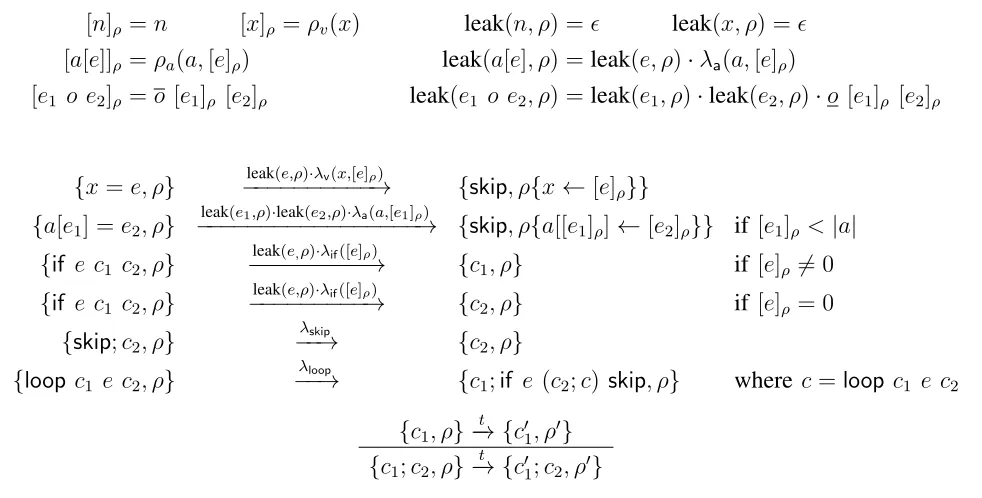
The interpretation [e]ρ and leakage leak(e, ρ)of an expression e in an environment ρ are elements of

Z and _L respectively. Figure 2 defines the functions formally. The evaluation of variables and constants generates no leakage; for operators, the leakage corresponds to the leakage of subexpressions and the specific leakage of the operation o [e1]ρ [e2]ρ. Note that, as for other operators, the definition of leakage for array access is parametrized by a leakage function λa :A ×Z→ L.

States and semantics of commands. States are pairs of the form _{c, ρ} where c is a command and ρ

is an environment. We use s.cmd and s.env to denote the first and second component of a state. The instrumented semantics of commands is modelled by statements of the form _{c, ρ}−→ {t c0, ρ0}, and is parametrized by constants λskip, λloop ∈ L, functions λv : X ×Z → L, and λif : Z → L. We use the

standard notation _{·{· ← ·}} for updating environments.

The semantics is standard, except for the semantics of loops, and the definition of the leakage. The loop command loop c1 e c2 first executes c1 (unconditionally, as the do-while command), then evaluates e: if e evaluates to true (i.e. [e]ρ6= 0) the command c2 is executed and the loop command is evaluated w.r.t. the updated environment (as in the while-do), else if e evaluates to false (i.e. [e]ρ= 0) the command terminates immediately.

The leakage of a command is the leakage of the expressions evaluated during the execution of the command plus a specific leakage. For array assignment, the specific leakage depends of the address

λa(a,[e1]ρ). For conditionnal, the leakage depends of the branch taken.

The following lemma establishes that the instrumented semantics is deterministic, as required by our setting.

Lemma 3. For all states a, b, b0, if a−→t b and a→−t0 b0, then b =b0 and t =t0.

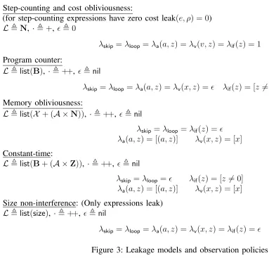
Leakage models. Figure 3 instantiates the functions for different leakage models. We use the notation

[n]ρ=n [x]ρ=ρv(x) leak(n, ρ) = leak(x, ρ) =

[a[e]]ρ=ρa(a,[e]ρ) leak(a[e], ρ) =leak(e, ρ)·λa(a,[e]ρ)

[e1 o e2]ρ=o [e1]ρ [e2]ρ leak(e1 o e2, ρ) =leak(e1, ρ)·leak(e2, ρ)·o [e1]ρ [e2]ρ

{x=e, ρ} −−−−−−−−−−→leak(e,ρ)·λv(x,[e]ρ) {skip, ρ{x←[e]ρ}} {a[e1] =e2, ρ}

leak(e1,ρ)·leak(e2,ρ)·λa(a,[e1]ρ)

−−−−−−−−−−−−−−−−−→ {skip, ρ{a[[e1]ρ]←[e2]ρ}} if [e1]ρ <|a| {if e c1 c2, ρ}

leak(e,ρ)·λif([e]ρ)

−−−−−−−−−→ {c1, ρ} if [e]ρ 6= 0

{if e c1 c2, ρ}

leak(e,ρ)·λif([e]ρ)

−−−−−−−−−→ {c2, ρ} if [e]ρ = 0

{skip;c2, ρ}

λskip

−−→ {c2, ρ}

{loop c1 e c2, ρ}

λloop

−−→ {c1;if e (c2;c) skip, ρ} where c=loop c1 e c2

{c1, ρ} t −

→ {c0₁, ρ0} {c1;c2, ρ}

t − → {c0

1;c2, ρ0}

Figure 2: Instrumented semantics of the while language

Instantiating the general setting. In order to complete the instantiation of the general setting, we must

additionally provide the definition of S(I) and f inal. These are respectively defined as the sets of states of the form _{S, ρ_} and _{skip, ρ_}, where ρ ranges over environments. Under these definitions, we can prove the aforementioned implications between the different policies.

Policies. Policies considered in the literature are generally of the form (=,. =), where =. represents low

equivalence, and is defined relative to a security lattice and a security environment. We consider a lattice with two security levels: H, or high, for secret and L, or low, for public. Then, a security environment is a mapping from variables and arrays to security levels. Finally, two environments ρ and ρ0 _{are low} equivalent w.r.t. a security environment Γ iff they map public variables and arrays to the same values, i.e. ρv(x) =ρ0v(x) for all variables x such that Γ(x) =L andρa(a, i) =ρ0a(a, i) for all arrays a such that Γ(a) = L and every i∈N.

2.3. Secure compilation

The problem addressed in this paper is an instance of secure compilation. It can be stated as follows: given source and target languages (with potentially different leakage monoids), a compiler _J·K from source to target programs, and two policies (φ, ψ) and (φ, ψ0_):

∀S. S _|= (φ, ψ)_∧safe(S) =_⇒? _JS_K|= (φ, ψ0)

Step-counting and cost obliviousness:

(for step-counting expressions have zero cost leak(e, ρ) = 0) L,N, _·,+,,0

λskip=λloop=λa(a, z) =λv(v, z) = λif(z) = 1

Program counter:

L,list(B),_·,++, ,nil

λskip=λloop=λa(a, z) =λv(x, z) = λif(z) = [z 6= 0]

Memory obliviousness:

L,list(X + (A ×N)), _·,++, ,nil

λskip=λloop =λif(z) = λa(a, z) = [(a, z)] λv(x, z) = [x]

Constant-time:

L,list(B+ (A ×Z)),_·,++,,nil

λskip =λloop= λif(z) = [z 6= 0] λa(a, z) = [(a, z)] λv(x, z) = [x]

Size non-interference: (Only expressions leak) L,list(size),_·,++, ,nil

λskip =λloop =λa(a, z) = λv(x, z) =λif(z) =

Figure 3: Leakage models and observation policies

support the same notion of leakage. The failure of the naive strategy forces us to consider an alternative strategy based on 2-simulations, which we develop in the following sections.

Since the set of input parameters is shared among all the compilation phases, we also assume that we have a precondition φ which is shared by all the phases.

3. Lockstep constant-time simulations

We present a simple method for proving preservation of observational non-interference, corresponding to lockstep simulations. Moreover, we instantiate our method to constant folding and spilling. Refinements of the method to manysteps and general simulations are provided in the next sections.

3.1. Non-cancellation of leakage

Program counter:

L,list(B+_{•}), _·,++, ,nil

λskip=λloop=λa(a, z) =λv(x, z) = [•] λif(z) = [z 6= 0]

Constant-time:

L,list(B+ (_{A ×}Z) +_{•}), _·,++, ,nil

λskip=λloop= [•] λif(z) = [z 6= 0] λa(a, z) = [(a, z)] λv(x, z) = [x]

Figure 4: Non-cancelling program counter and constant-time

• for every t1, t01 ∈ Latomic and t2, t02 ∈ L,

t1·t01 =t2·t02 =⇒ t1 =t2∧t01 =t02

• for every t∈ Latomic and t0 ∈ L, t·t0 6=

The non-cancellation property entails the following useful property.

Lemma 4. Assume ψ is non-cancelling. Then for every t1, . . . , tm, t01, . . . , t0n∈ Latomic,

t1·. . .·tm =t01 ·. . .·t0n ⇒m=n∧

^

1≤i≤n

ti =t0i

It turns out that none of leakage models from Figure 3 satisfies the non-cancelling condition. However, one can easily define alternative leakage models that verify the non-cancelling condition, and which yield equivalent notions of non-interference. For instance, Figure 4 presents alternative models for the program counter and constant-time policies; informally, the non-cancelling leakage models are obtained by replacing leakages by a leakage[_•], where _•is a distinguished element, to record that one execution step has been performed.

3.2. General framework

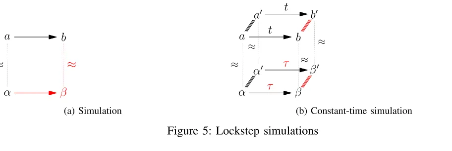
We start by recalling the standard notion of simulation from compiler verification. In the simplest (lockstep) setting, one requires that the simulation relation relates one step of execution of S with one step execution of C, as shown in Figure 5a, in which black represents the hypotheses and red the conclusions. The horizontal arrows represent one step execution of S from state a to state b, and one step execution of C from state α to state β. The relation _{· ≈ ·}relates execution states of the source and of the target program.

Definition 5 (Lockstep simulation). _≈ is a lockstep simulation when:

• for every source step a→b, and every target state α such that a≈α, there exist a target state β and a target execution α →β such that end states are related: b ≈β;

• for every input parameter i, we have S(i)≈C(i);

The following lemma follows from the assumption that all our languages have a deterministic semantics.

Lemma 5. Assume that _≈ is a simulation. Then for every target execution step α_→β and safe source

state a such that a_≈α, there exists a source execution step a_→b such that b _≈β.

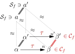
Our method is based on constant-time simulations, a new proof technique adapted from the simulation technique in compiler verification. Whereas simulations are proved by 2-dimensional diagram chasing, constant-time simulations are proved by 3-dimensional diagram chasing. Figure 5b illustrates the definition of constant-time simulation, for the lockstep case. It introduces relations _{· ≡}S · and· ≡C · between source and target states, depicted with a triple line in the diagram. Horizontal arrows represent one step executions (as before), but we now consider two executions at source level and two executions at target level.

Definition 6 (Lockstep 2-simulation). (_≡S,≡C) is a lockstep 2-simulation with respect to ≈ iff

• For every source steps a−→t b and a0 −→t b0 such that a ≡S a0 and for every target steps from α−→τ β and α0 _−→τ0 _β0 _{such that a ≈ α and a}0 _≈α0 _{and α ≡}

C α0 and b ≈ β and b0 ≈β0, we have b ≡S b0 and β ≡C β0 and τ =τ0;

• For every pair of input parameters i, i0 s.t. φ i i0, we have S(i)≡S S(i0) and C(i)≡C C(i0).

The notion of constant-time simulation is tailored to make the _{· ≡ ·} relation inductive, and to yield preservation of (both variants of) observational non-interference. This is captured by the next theorem, where φ is the relation on input parameters —it is useful to think about φ as low-equivalence between memories—and _≡S and ≡C are two relations on source and target states–it is useful to think about ≡S and _≡C as equivalence of code pointer, i.e. the two states point to the same instruction.

Theorem 1 (Preservation of constant-time policy). Assume that leakage is non-cancelling. Let S be a

safe source program and C be the target program obtained by compilation. If S is TIONI (resp. TSONI) w.r.t. (φ,=) then C is TIONI (resp. TSONI) w.r.t. (φ,=), provided the following holds:

1) _≈ is a lockstep simulation;

2) (_≡S,≡C) is lockstep 2-simulation w.r.t. ≈. Proof sketch. Consider two target executions

α1 τ1

−→. . . τm

−→αm+1 α10 τ0

1

−→. . . τn0 −→ α0_n+1

starting in related states, i.e. φ α1 α01, and such that αm+1 and α0n+1 are final states. We must show that m=n andτi =τi0 for every 1≤i≤n. By safety of S and 1) and Lemma 5, there exist source executions

a1 t1

−→. . . tm

−→am+1 a01 t01

−→. . . t0n −→a0_n+1

such that φ a1 a01 and ai ≈αi for every 1≤i≤m+ 1 and a0i ≈αi0 for every 1≤i≤n+ 1. Moreover, by 1) am+1 and a0n+1 are final states, and by 2) α1 ≡C α10 and a1 ≡S a01. By the constant-time property ofS, and the non-cancelling property of leakage,m =n and ti =t0i for every 1≤i≤n. We next reason by induction on i, applying 2) to conclude that αi ≡C α0i and ai ≡S a0i and τi =τi0, as desired.

a

α

b

β

≈ ≈

(a) Simulation

a

α

b

β a′

α′

b′

β′

≈ ≈

≈ ≈

t t

τ τ

(b) Constant-time simulation

Figure 5: Lockstep simulations

independently. This separation of concerns limits the proof effort and support modular proofs. In particular, when the compiler is already proved correct (by showing a simulation _≈), one only needs to show that there exists a constant-time simulation w.r.t. _≈.

3.3. Discussion

Theorem 1 and its subsequent generalizations (Theorem 4 and Theorem 6) are broadly applicable to settings where both the source and target policies are strengthenings of the program counter policies. This limitation is best explained by an analogy with unwinding lemmas, a standard technique for proving information flow policies. However, we stress that the analogy is given for explanatory purposes only; in particular, our method for proving preservation of observational non-interference is modular and oblivious to the choice of a relationφ and of the method used for proving observational non-interference.

Informally, unwinding lemmas come in two flavours: “locally preserves” unwinding lemmas show that two executions started in related states yield related states, where the notion of related states is given by a low-equivalence relation akin to φ, and “step-consistent” unwinding lemmas show that under some conditions, one step execution yields related states, i.e. a→a0 implies that a and a0 are low-equivalent. “Step-consistent” unwinding lemmas are used for reasoning about diverging control flow, i.e. when programs branch on secrets, and are not required when executions have the same control flow, as imposed by the program counter policy. Our methods only consider the equivalent of “locally preserves” unwinding lemmas, and are therefore restricted to policies that entail program counter security. It is certainly possible to extend our method to provide a counterpart to the “step-preserving” policies. However, it remains an open question whether the general framework could still be instantiated to a broad class of program optimizations.

3.4. Examples

3.4.1. Constant folding. We illustrate the general scheme for proving preservation of the constant-time

We use the lockstep simulation technique to prove that constant-folding preserves the constant-time policy. Our first step is to prove that the constant-folding satisfies the lockstep diagram for simulation. To this end, we consider the relation a≈α is defined by

Ja.cmdK =α.cmd∧a.env=α.env

Lemma 6. The relation _≈ is lockstep simulation invariant.

The proof of this lemma is based on the fact that if an expression e has a semantics in a given environment ρ (i.e. [e]ρ=n) then its compilation has the same semantics, [JeK]ρ=n.

Our next step is to prove that the transformation satisfies the lockstep diagram for constant-time simulation. To this end, we use for the _≡ relations the equality of commands a _≡c a0 _{defined by}

a.cmd=a0.cmd.

Lemma 7. (≡c,≡c) is a lockstep 2-simulation w.r.t. _≈.

The proof of this lemma is based on the fact that if an expression e has a (leaky) semantics in both environments and the leakages coincide (i.e. [e]ρ=n and [e]ρ0 =n0 and leak(e, ρ) = leak(e, ρ0)), then

the compilation of e generates the same leakage in both environments, i.e.

leak(JeK, ρ) = leak(JeK, ρ

0₎

It follows that constant folding preserves the constant-time property.

Theorem 2. Constant-folding preserves the constant-time policy.

3.4.2. Register allocation. Register allocation is a compilation pass that maps an unbounded set of

variables into a finite set of registers. In order to preserve the semantics of programs, it is often necessary that the target program stores the value of some variables on the stack, effectively turning variable accesses into memory accesses. Formally, register allocation produces for every program point a mapping from program variables to registers or stack variables (interpreted as an integer denoting the relative position in the stack). Finding optimal assignments that minimize register spilling is a hard problem, and is commonly solved using translation validation. Specifically, computing the assignment is performed by an external program, and a verified checker verifies that the assignment is compatible with the semantics of programs. Formally, we modify the language and its semantics to distinguish between regular variables r and stack variables k . The notion of state changes accordingly, i.e. the environment is now a partial map from registers and stack position to values. The semantics of the language is modified accordingly; in particular, each read/write into the stack leaks its position.

leak(k, ρ) = [k]

leak_{k=e;c, ρ_}=leak(e, ρ) ++ [k]

We let σ be the assignment output by register allocation.

Proving the correctness of register allocation is relatively easy. The proof relies the correctness of the liveness analysis which underlies register allocation. Preservation of the constant time policy is more interesting, because spilling introduces new memory reads and writes. The crucial observation is that the addresses leaked by spilling do not depend on the memory, since they are constant offset relative to the top of the stack. Thus, the proof of the 2-simulation diagram does not pose any specific difficult. For both proofs, we use a_≈α defined by

+ a

α

b

β

≈ ≈

(a) Simulation

a

α

b

β a′

α′

b′

β′

n n′

≈

≈

≈ ≈

t t

τ τ

(b) Constant-time simulation

Figure 6: Manysteps simulations

Theorem 3. _≈ is lockstep simulation invariant. (_≡c,_≡c) is a lockstep 2-simulation relative to_≈. Variable

spilling preserves the constant-time policy.

Remark 1. Following [5], our formalization separates register allocation in two steps. The first step

performs some form of variable renaming and defines for every program point a mapping from source variables to target variables. The second step performs spilling, and defines a single, global, mapping from variables to variables or stack variables. Furthermore, the mapping must be the identity for variables that are mapped to variables.

This proof can be extended to a more complex language with function calls and stack pointer. The difficulty here is that a stack address will not be a constant k but relative to the top of the stack stk+k. Then, when proving preservation of constant-time we have to show that introduced leaks are equal in two different executions, i.e. stk1 +k = stk2 +k where stki correspond to the value of the stack pointer in execution i. So we have to ensure equality of stack pointers. This can be done by a small modification of _≡ predicate of the target language, so that it imposes equality of commands and of stack pointers. Since the value of the stack pointer only depends on the control flow of the program and that preservation of constant-time already requires equality of the control flow, establishing equality of stack pointers adds no difficulty.

4. Manysteps constant-time simulations

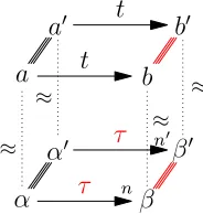
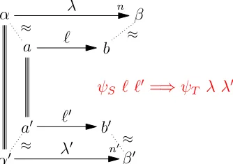
The requirement of lockstep execution is often too strong in practice. For illustrative purposes, consider the nonsensical transformation that replaces every atomic instruction i by skip;i. Every single execution step of the source program will correspond to two execution steps of the target program (so it does not correspond to the lockstep simulation). There exist alternative notions of simulations which relax the requirement on lockstep executions by allowing more than one step of execution (i.e. manysteps), as shown on Figure 6a. We show that an equivalent relaxation exists for 2-simulations.

4.1. Framework

to the same state. A simulation relation will necessarily relate the source state to some target state α, and given the hypotheses of the constant-time simulation diagram (a _≈α, a_→a, and α_→+ _{α) it is} generally not possible to tell how many loop iterations separate the two occurrences of the target state α

(hence to prove that any two such target executions have the same length).

To overcome this issue, the simulation diagram is refined to predict how many steps of the target will correspond to each step of the source. This information is usually implicit in the simulation proof; we only make it explicit to be used in the constant-time simulation diagram.

Formally, we introduce a function num-steps(a, α) which, assuming that a and α are two reachable states related by the simulation relation, predicts how many steps of the target semantics are to be run starting from α to close the manysteps simulation diagram.

Definition 7 (Manysteps simulation). _≈ is a manysteps simulation w.r.t. num-steps when:

• for every source steps a−→b, and every target state α such that a≈α, there exist a target state β and target execution α−→n_{β, where n =num-steps(a, α), such that end states are related: b ≈β;} • for every input parameter i, we have S(i)_≈C(i);

• for every source and target states b and β such that b ≈β, we have b is a final source state iff β is a final target state.

Given such a simulation diagram, it is possible to build the constant-time simulation diagram that universally quantifies over two instances of this diagram, as depicted on Figure 6b. The diagram reads as follows.

Definition 8 (Manysteps 2-diagram). A pair of relations (_≡S, ≡C) is a manysteps 2-simulation w.r.t. ≈

and num-steps iff the following holds: for all a, a0, b, b0, α, α0, β, β0, t, τ, τ0 such that

• initial states are related a_≡S a0 and α ≡C α0; • a−→t b and a0 _−→t _b0_;

• α−→τnβ and α0 τ

0

−→n0

β0 _{where n =num-steps(a, α) and n}0 _=num-steps(a0_{, α}0_); • the simulation relation holds a≈α,a0 ≈α0, b≈β, and b0 ≈β0

we have

• equality of leakage τ =τ0 and n =n0, • final states are related b ≡S b0 and β ≡C β0.

This definition, together with a condition on initial states, enable us to define the manysteps constant-time simulation.

Definition 9 (Manysteps 2-simulation). A pair of relations (_≡S,≡C) is amanysteps 2-simulation relative

to _≈ w.r.t. num-steps when:

1) (≡S,≡C) satisfy the manysteps 2-diagram w.r.t. ≈ and num-steps;

2) for every pair of input parameters i, i0 s.t. φ i i0, we have S(i)≡S S(i0) and C(i)≡C C(i0).

Theorem 4 (Constant-time preservation from manysteps 2-simulation). Assume that leakage is

non-cancelling. Let S be a safe source program and C be the target program obtained by compilation. If S

is TIONI (resp. TSONI) w.r.t. (φ,=) then C is TIONI (resp. TSONI) w.r.t. (φ,=), provided the following

holds, for a given num-steps function that is strictly positive: 1) _≈ is a manysteps-simulation w.r.t. num-steps;

4.2. Example: Expression flattening

The flattening of expressions models the transformation to a 3-address code format: each expression is split in a sequence of assignments and a final expression such that at most one operator appears in each expression. This actually fixes the evaluation order of the sub-expressions. Since the evaluation of an expression is done, after transformation, in several steps, the leakage corresponding to an expression is spread among the leakages of these steps.

The transformed program may use additional variables to store the values of some sub-expressions. Therefore, the set of program variables is extended with names for such temporary values.

The procedure that flattens an expression e is written F(e): it returns a pair (p, e0_{) where p is a} prefix command and e0 an expression such that the evaluation of p followed by the evaluation of e0

yields the same value as the evaluation ofe; moreover, the evaluation of ponly modifies fresh temporary variables. The transformation_J·K of a program applies F to each expression e occurring in that program and inserts the corresponding prefix just before, as follows—we note (p, e0_{) =F(e):}

Jx=eK = p;x=e

0

Jif e c1 c2K = p;if e0 Jc1K Jc2K Jloop c1 e c2K = loop (Jc1K;p) e0 Jc2K

Note here that the loop structure of our language conveniently allows not to duplicate the sequence p, as arbitrary instructions can be executed before the loop guard.

The correctness of this transformation states that the source and compiled programs agree on the values of the non-temporary variables. To this end, the relation a _≈ α between states is defined as follows:

Ja.cmdK=α.cmd∧ ∀x, a.env(x) = α.env(x)

where xdenotes a original program variable (i.e. not a temporary variable introduced by the compilation). The target command is the result of the compilation of the source command and the source and target memories agree on the values of the non-temporary variables.

To show that this relation is a simulation, we must predict the number of target steps corresponding to each source step. For each states a and α, we define num-steps(a, α) as 1 +n, wheren is the length of the prefix of the expression that is evaluated during the step starting in a (if any). By construction, this function is strictly positive. To prove that this pass preserves constant-time, we build a manysteps 2-simulation diagram.

Theorem 5. The relation_≈is a manysteps simulation w.r.tnum-steps. (_≡c,_≡c) is a manysteps 2-simulation

relative to _≈ w.r.t num-steps. Expression flattening preserves the constant-time policy.

The main argument is that if the evaluations of two expressions produce the same leakage, then evaluations after flattening also produces the same leakage. Notice that this transformation may choose any evaluation strategy for the expressions, and that needs not be related to the order that appears in the definition of the leakage of expressions.

5. General constant-time simulations

5.1. Framework

a Sf ∋

α β ∈ Cf

a′ Sf ∋

α′ β′ _{∈ Cf} n

n′

≈ ≈

≈ ≈

τ τ

Figure 7: Final 2-diagram

the full source program (and not only the current step) is constant-time. Formally, the definition of the manysteps 2-diagram is complemented with additional hypotheses: initial source states a and a0 _are reachable in S and are a constant-time pair of states; initial target states α and α0 _{are reachable in C.} Finally, we relax the condition on final state in the simulation: when the source execution terminates the target execution is allowed to take a few more steps.

To allow num-steps to be zero, the simulation diagram features an additional constraint: there should be no infinite sequence of source steps that are simulated by an empty sequence of target steps (every source state in the sequence being in relation with a single one target state). This constraint is usually formalized by means of a measure of source states which strictly decreases whenever the corresponding target state stutters.

Definition 10 (General simulation). Given a relation _≈ between source an target states, a function _{| · |}

from source states to natural numbers2, and a function num-steps from pairs of source and target states to natural numbers; we say that _≈ is a general simulation w.r.t. _{| · |} and num-steps when:

• for every source step a→b and every target state α such that a≈α, there exist a target state β and a target execution α −→n_{β where n =num-steps(a, α) such that end states are related: b≈β;} • for every source step a→b and every target state α such that a≈α and num-steps(a, α) = 0, the

measure of the source state strictly decreases: _|a_|>_|b_|;

• for every final source state a and every target state α such that a≈α, there exist a final target state

β and a target execution α_−→n_{β where n =num-steps(a, α) such that end states are related: a≈β.}

To allow the target execution to terminate after the source execution, we introduce the following variant of the 2-simulation, depicted on Figure 7.

Definition 11 (Final 2-diagram). A pair of relations (_≡S, ≡C) satisfy the final constant-time diagram

w.r.t. _≈ and num-steps when the following holds: for all a, a0_,α,α0_{, β,β}0_{,τ, τ}0 _{such that:} • initial states are related a≡S a0, α≡C α0;

• initial source states are final a, a0 ∈ Sf;

• there are two target executions α −→τ nβ and α0 τ

0

−→n0_β0 _{where n = num-steps(a, α) and n}0 ₌ num-steps(a0_{, α}0_);

• the simulation relation holds a≈α,a0 ≈α0, a≈β, and a0 ≈β0

we have

• equality of leakage τ =τ0 and n =n0;

Jif 0 c1 c2K=Jc2K

Jif b c1 c2K=if b Jc1K Jc2K if b6= 0 Jloop c1 0 c2K=Jc1K

Jloop c1 b c2K=loop Jc1K b Jc2K if b6= 0

Figure 8: Removal of trivial (false) branches

• end states are related and final β ≡C β0, β, β0 ∈ Cf.

Definition 12 (General 2-simulation). Given a relation _≈, a function _{| · |}, and a function num-steps as

above, we say that the pair of relations (_≡S,≡C) is a (general) 2-simulation when: 1) (_≡S,≡C) satisfy the manysteps 2-diagram w.r.t. ≈ and num-steps;

2) for every pair of input parameters i,i0 _{s.t. φ i i}0_{, we have S(i)≡}

S S(i0) and C(i)≡C C(i0); 3) for all related source states a≡S a0, none or both of them are final: a∈ Sf ⇐⇒ a0 ∈ Sf; 4) (_≡S,≡C) satisfy the final 2-diagram w.r.t. ≈ and num-steps.

Theorem 6 (Constant-time preservation from general 2-simulation). Assume that leakage is

non-cancelling. Let S be a safe source program and C be the target program obtained by compilation. If S

is TIONI (resp. TSONI) w.r.t. (φ,=) then C is TIONI (resp. TSONI) w.r.t. (φ,=), provided the following

holds, for given num-steps and _|·| functions:

1) _≈ is a general simulation w.r.t. _|·| and num-steps;

2) (_≡S,≡C) is a general 2-simulation w.r.t. ≈, |·|, and num-steps.

Remark 2. In the Coq formalization, we use slightly more convenient definitions in which more

hypotheses are available: all considered states are reachable, initial source states (a and a0_{) are a} constant-time pair of states. This enables to do more modular proofs.

5.2. Examples

5.2.1. Dead branch elimination. In this section, we present a transformation that we designed for the

purpose of illustration: a more general and less artificial version will be discussed in the following section. This transformation removes conditional branches whose conditions are trivially false. More precisely, the compilation function _J·K is defined as depicted on Figure 8. Assignments are kept unchanged; the if

instructions whose conditions are trivially false (i.e., the literal 0 is used as guard) are replaced by their else branch (recursively compiled); similarly, loop instructions whose guard is false are removed: only the first part of the loop body is kept (recursively compiled).

To justify the correctness of this transformation, we define a relation a_≈α between source state a

and target state α as: α = {Ja.cmdK, a.env}; the target command is the compilation of the source

command, and both states have the same environment.

conditional on false (if or loop), we also define a measure _|a_| of source execution states by taking the full size of a.cmd, such that this measure strictly decreases when the target takes no step.

Theorem 7. _≈ is general simulation invariant.(≡c,≡c)is a general 2-simulation relative to_≈, num-steps

and _|·|. Dead branch elimination preserves the constant-time policy.

5.2.2. Constant propagation. A slightly more interesting variant of the previous transformation is

constant propagation: a static analysis prior to the compilation pass infers at each program point, which variables hold a statically known constant value; then using this information, each expression can be simplified (as in the constant folding transformation described in _§ 3.4.1) and the branches that are trivial after this simplification can be removed.

This transformation, as many other common compilation passes, relies on the availability of a flow-sensitive analysis result: some information must be attached to every program point. As usual, since our language has no explicit program points, we enrich its syntax with annotations. More precisely, each instruction gets one annotation, except the loop which gets two: one that is valid at the beginning of each loop iteration, and one that is valid when evaluating the loop guard. The small-step semantics, when executing a loop, introduces an if and a loop. The annotations to put on the next iteration may depend on the purpose of these annotations; therefore, the semantics is parametrized by a annot-step function which describes how to compute the annotations of a loop at the next iteration, yielding the following rule for the execution of the loop instruction (decorated lettersk figure the annotations):

{loopk1

k2 c1 b c2, ρ} → {c1;if k2 _{b (c}

2;loop k0

1 k0

2 c1 b c2) skip, ρ} where (k0

1, k02) =annot-step(k1, k2).

In this particular case of constant propagation, we assume that the source program is annotated with partial mappings from variables to constant values (integers). Those annotations are generated by a first pass of analysis and are certified independently. Given this information, the compilation may simplify expressions, remove if whose guard is trivial, and remove loops whose guard is false.

However, the compilation only transforms constructs that syntactically appear in the program source code and does not operates on the constructs that are in the execution state as a result of the semantic execution of the program. In particular, the compilation will not transform a trivial if that results from the execution of a loop whose guard is trivially true. More generally, a compilation pass may apply different transformations to similar pieces of code depending on some heuristic, and these heuristics should be irrelevant to the correctness argument. To overcome this issue we reuse the annotation facility to be able to statically determine how each source instruction is transformed. The compiler generates two programs: an annotated version of the source3 and its compiled version. The compiler adds a boolean flag to the source to tell whether a branch is eliminated or not. Therefore, trivial branches that only appear during the execution and are not visible to the compiler will not have this flag set and the num-steps function can predict that the corresponding execution step is preserved. The flag part of k2 is false indicating that the if is preserved; the annot-step function is the identity. The num-steps function is defined following the same idea of the previous example. As well, to prove that execution does not stutter for ever we use the size of the command. The _≈ predicate ensures equality of environments and that the target code come from the compilation of the source taking into account the flags.

Theorem 8. _≈ is general simulation invariant.(≡c,≡c)is a general 2-simulation relative to_≈, num-steps

and _|·|. Constant-propagation preserves the constant-time policy.

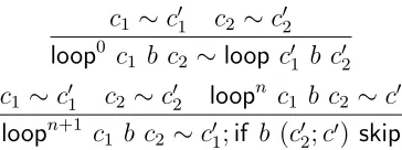
c1 ∼c01 c2 ∼c02

loop0 c1 b c2 ∼loop c01 b c02

c1 ∼c01 c2 ∼c02 loopn c1 b c2 ∼c0

loopn+1 c1 b c2 ∼c01;if b (c02;c0) skip

Figure 9: Specification of loop peeling

5.2.3. Loop peeling. Loop peeling is an optimization that unrolls the first iterations of loops. It is a

good example where annot-stepis not the identity function but counts the number of loop iterations. How many iterations are actually peeled may depend on heuristics which should not be visible in the correctness proof (nor in the simulation argument). In this case, instead of proving one particular compilation scheme, we define a relation between source and target commands that captures various possible ways to perform the transformation. This relation is written _∼ and defined on Figure 9. Each source loop instruction is annotated with a number stating how many iterations of this loop are peeled. For these annotations to remain consistent during the execution, this counter is decremented on each iteration: formally, annot-step(n, a) = (max(0, n−1), a).

For this transformation, the _≈ predicate is equality of environments and _∼ of commands. The num-steps function is equal to 1, except on loop with a non-zero annotation for which it is 0. The _|·| function is the number of nested loop in the first instruction.

Theorem 9. _≈ is simulation invariant. (≡c,≡c) is a 2-simulation relative to _≈, num-steps and _|·|. Loop

peeling preserves the constant-time policy.

5.2.4. Linearization. Linearization transforms programs into lists of instructions with explicit labels.

The linear language features (only) two instructions: assignment “x=e” of the value of an expression e

to a l-value x; and conditional branching “jnzb n”, which continues execution at (relative) position n

when expression b evaluates to a non-zero value or falls through the next instruction otherwise. When the condition is syntactically 1, we simply write “goto n”. In this language, a program is a list of instructions, and execution starts at position zero, i.e., at the beginning of said list. The execution state is a triple made of the program counter, the current environment, and the whole program.

In the language, the leakage of a step correspond to the leakage of the expressions and the value of the next program point. This is analogous to leaking the boolean value of conditional jumps.

The transformation _J·K from the structured language from previous sections to linear is described in Figure 10. It introduces forward jumps at the end of else branches (to bypass the corresponding then branches) and at the beginning of loops (to bypass the second body before the first iteration). These jumps do not correspond to any particular instruction in the source. To define the _≈ relation for the correctness proof, we always allow the target execution to perform (any number of) such jumps. The technical difficulty of the proof comes from the fact that source instruction will be in relation with many target instructions, some of them correspond to the compilation of the original instruction but some of them come from its context; breaking the locality of the proof.

Jx=eK =x=e

Jif b c1 c2K =jnz b n2;Jc2K;goto n1;Jc1K

// where n2 =|Jc2K|+ 2 and n1 =|Jc1K|+ 1

Jloop c1 b c2K =goto n2;Jc2K;Jc1K;jnz b n

// where n2 =|Jc2K|+ 1 and n=−|Jc2K;Jc1K|

Figure 10: Linearization

To establish the 2-simulation, we introduce a relation _≡L between states that claims that the program point is the same. The proof of the 2-diagram follows without surprises. The technicalities due to the change in representation (from a structured language to an unstructured one) are dealt with using the same lemmas as for the correctness proof.

The num-steps function is defined as the number of forward jump from the current target program counter plus 1 if the current source instruction is not a loop. The _|·| function is the number of nested loops in the first source instruction.

Theorem 10. The relation _≈ is a simulation w.r.t num-steps. (_≡, _≡L) is a 2-simulation relative to _≈

w.r.t. num-steps and _|·|. Linearization preserves the constant-time policy.

5.2.5. Common branches factorization. In these last two sections, we consider a new kind of

trans-formation where the order of evaluation of expressions/instructions is changed. The first transtrans-formation consists in factorizing the common prefix of conditional branches. In other terms, the transformation will replace a statement of the form if e (h;c1) (h;c2) by h;if e c1 c2, when the evaluation of e is not affected by the evaluation of c. This allows to reduce the size of the code. To prove the correctness, we need to establish the general simulation for a given relation _≈. When the if instruction on e is executed in the source program, the h instructions should be first executed in the target program before executing the conditional on e. Similarly, when the c instructions are executed in the source program, they have been already executed in the target program, so nothing should be done. For the correctness of the compiler the difficulty is that environment of the source program and of the target program are desynchronised at some point. For 2-simulation the difficulty is that leaks of h will appear in the target trace before they appear in the source. In particular the trace t corresponding to the leak of the if e

does not contain the leaks of h, so we should be able to prove that the leaks of h will be equal in both evaluations because the source program in constant-time.

The notion of simulation used for this transformation a ≈α is defined by:

∃h, a.cmd_∼h α.cmd_{∧ {}a.env, h_{} →}∗ _{α.env,skip_}

The predicate c _∼h c0 _{is presented Figure 11. Morally c is the code of the source program, c}0 _{of the} target program, and h is the sequence of instructions which have been already executed in the target program but are still to be executed in the source. The notion of simulation requires that the evaluation of h in the source environment terminates on the target environment. When h=skip we omit it.

c1 h

∼c0₁ c2 h

∼c0₂ terminating(h) write(h)∩read(e) =∅

if|h|+1 e c1 c2 ∼h;if e c01 c02

c∼h c0

i0;ci_∼;h c0

Figure 11: _≈ predicate for common branches elimination

number indicates the value of the num-steps function needed by the simulation. For conditional, if the number is not 0, it corresponds to the number of instructions which have been factorized out by the compiler. The code of each branch should be related by _∼h, h should be terminating4 _{and should not}

modify the variables read by e (this ensures that the evaluation of e can swap with the evaluation of h). If h is not skip, see the last rule, it means that the target program has already executed h and the source program should catch up with the target. This means that the source evaluation step corresponds to no execution step in the target program; this is why the annotation in the source is 0.

The num-steps function cannot be fully inferred statically (i.e., at compile time), because h may contain conditionals and so the number of steps to execute depends on the execution environment and of which branches are taken. It is not a problem with our proof technique since the num-steps function is parametrized by the source and the target states. The termination condition ensures that the evaluation of h will terminate in a finite number of steps5. The _|·| function is the size of the source instruction.

Theorem 11. _≈ is general simulation with w.r.t._|·| and num-steps .(_≡c,_≡c) is a general 2-simulation

relative to _≈. Common branches factorization preserves the constant-time policy.

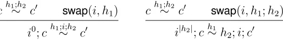
5.2.6. Switching instructions. Switching instructions of a program is a very common optimization. It

can be used together with common branches to improve its efficiency, but its most common use is for instruction scheduling. It is a typical example of transformation that depends on heuristics (which can be different for each target architecture) which should not be visible in the correctness proof. To that end, we simply prove a checker taking a source program and a target program and returns true if they are equal up to a valid permutation inside basic blocks (list of assignments), but the control-flow is still the same. The notion of valid permutation should ensure that the semantic of the program is unchanged. For example, c1;c2 can be transformed into c2;c1 if variables read and written by c2 are not written by c1 (and vice versa), furthermore both instructions should terminate6. To be able to define the _≈ relation we encounter the same difficulty as for common branches factorization: the source and target states are not synchronized. Figure 12 defines the _∼ predicate used to define _≈. As for common branches factorization it is parametrized by a code h representing instructions already executed in the target and that remain to be executed in the source. Intuitively, c_∼h c0 _{should be interpreted has c is a} valid permutation of h;c0_{. Some rules (not shown) allow to perform transformation under context, the} two presented rules define the permutation. The predicate swap ensures that the two instructions can be safely swapped without changing the semantic of the program. The num-steps function return directly the annotation of the current instruction, the _|·| is the size of the instruction.

4. Our formalization requires thathis a sequence of assignments and conditionals. It would be possible to support loops for which the compiler is able to prove termination.

5. Without that condition it is not clear that the correctness of the compiler can be expressed/proved using a small step simulation diagram.

6. Termination ofc1 is needed to ensure preservation of non-interference: ifc1 is non-terminating thenc1;c2 can be aTSONIprogram

ch1;h2

∼ c0 swap(i, h1)

i0;ch1;i;h2 ∼ c0

ch1;h2

∼ c0 swap(i, h1;h2)

i|h2|_;ch_∼1 _h 2;i;c0

Figure 12: _≈ predicate for switching instructions

Theorem 12. _≈ is a general simulation w.r.t. num-steps and _|·|. (_≡c,_≡c)is a 2-simulation relative to _≈.

Switching instructions preserves the constant-time policy.

6. Related work

Many recent works address the challenge of verifying constant-time implementations formally, using established methods such as type systems, abstract interpretation and deductive verification. These methods are applied to source programs [10], assembly programs [6], or intermediate representations (e.g. LLVM IR) [4], [25]. These works do not address the problem of policy-preserving compilation—see however the informal discussion in [4]. Preservation of the constant-time policy by compilation is discussed explicitly in [5], where Almeida et al provide an informal argument for the Jasmin compiler; our method provides the means to make their proof formal. Independently, preservation of the constant-time policy by compilation is studied in [24], where Protzenko et al. claim that their translation from

λow* to C* preserves constant-time. We have been unable to reconstruct their argument, as it uses the usual notion of simulations. However, we believe that the notion of constant-time simulation can also be applied in their setting. Barthe et al [7] develop a general method for result-preserving compilation, and use their method to improve the precision of a constant-time analysis at intermediate level. However, their work focuses on preserving the results of alias analyses and does not study preservation of the constant-time policy. Almeida et al [3] give a simple translation validation technique to guarantee preservation of security in the program counter model for the CompCert compiler.

Other works have considered preservation of specific information flow policies by compilation. Barthe et al [8] define an information flow type system for a concurrent programing language and prove that typable programs are compiled into non-interfering assembly programs, under reasonable assumptions on the scheduler. Laud [17] and Fournet and Rezk [12] define information flow type systems for a core imperative language, and prove that programs are compiled into cryptographically secure implementations. Murray et al [21] prove preservation of value-dependent noninterference for a concurrent imperative language. Their proof uses coupling invariants, which are related to 2-simulations. However, they do not explicitly address the problem of preserving 2-properties by standard compilation passes.

Motivated by developing foundations for secure compilation, Patrignani and Garg [22] explore preservation of hyperproperties as an alternative to full abstraction. However, they do not propose general proof techniques for proving that specific compilation passes preserve a given hyperproperty.

7. Conclusion

We have developed a general method for proving preservation of software-based side-channel countermeasures by compilation, and provided instantiations to representative compiler optimizations. In our experience, proving preservation of constant-time policy is sometimes simpler than proving correctness of the transformation.

Additionally, we have formalized both the general methods and their instantiations using theCoqproof assistant. The overall development is over 8,000 lines of Coq code. The proofs of optimizations range from 250-300 lines (constant propagation and spilling) to 750-800 lines (code motion and expression flattening).

A natural target for future work is to apply our methods to existing verified compilers. Although our work is carried for a rather simple language, we are confident that our selection of optimizations covers the main difficulties that can appear when proving preservation of the constant-time policy for C like languages. In particular, we are confident that our methods are applicable to the Jasmin compiler.

References

[1] Martin R. Albrecht and Kenneth G. Paterson. Lucky microseconds: A timing attack on amazon’s s2n implementation of TLS. In Marc Fischlin and Jean-S´ebastien Coron, editors, Advances in Cryptology - EUROCRYPT 2016 - 35th Annual International Conference on the Theory and Applications of Cryptographic Techniques, Vienna, Austria, May 8-12, 2016, Proceedings, Part I, volume 9665 ofLecture Notes in Computer Science, pages 622–643. Springer, 2016.

[2] Nadhem J. AlFardan and Kenneth G. Paterson. Lucky thirteen: Breaking the TLS and DTLS record protocols. In 2013 IEEE Symposium on Security and Privacy, SP 2013, Berkeley, CA, USA, May 19-22, 2013, pages 526–540. IEEE Computer Society, 2013. [3] Jos´e Bacelar Almeida, Manuel Barbosa, Gilles Barthe, and Franc¸ois Dupressoir. Certified computer-aided cryptography: efficient provably secure machine code from high-level implementations. In Ahmad-Reza Sadeghi, Virgil D. Gligor, and Moti Yung, editors,

2013 ACM SIGSAC Conference on Computer and Communications Security, CCS’13, Berlin, Germany, November 4-8, 2013, pages 1217–1230. ACM, 2013.

[4] Jos´e Bacelar Almeida, Manuel Barbosa, Gilles Barthe, Franc¸ois Dupressoir, and Michael Emmi. Verifying constant-time implementations. In Thorsten Holz and Stefan Savage, editors,25th USENIX Security Symposium, USENIX Security 16, Austin, TX, USA, August 10-12, 2016., pages 53–70. USENIX Association, 2016.

[5] Jos´e Bacelar Almeida, Manuel Barbosa, Gilles Barthe, Arthur Blot, Benjamin Gr´egoire, Vincent Laporte, Tiago Oliveira, Hugo Pacheco, Benedikt Schmidt, and Pierre-Yves Strub. Jasmin: High-assurance and high-speed cryptography. InProceedings of the 24th ACM Conference on Computer and Communications Security(CCS), 2017.

[6] Gilles Barthe, Gustavo Betarte, Juan Diego Campo, Carlos Daniel Luna, and David Pichardie. System-level non-interference for constant-time cryptography. In Gail-Joon Ahn, Moti Yung, and Ninghui Li, editors,Proceedings of the 2014 ACM SIGSAC Conference on Computer and Communications Security, Scottsdale, AZ, USA, November 3-7, 2014, pages 1267–1279. ACM, 2014.

[7] Gilles Barthe, Sandrine Blazy, Vincent Laporte, David Pichardie, and Alix Trieu. Verified translation validation of static analyses. In

30th IEEE Computer Security Foundations Symposium, CSF 2017, Santa Barbara, CA, USA, August 21-25, 2017, pages 405–419. IEEE Computer Society, 2017.

[8] Gilles Barthe, Tamara Rezk, Alejandro Russo, and Andrei Sabelfeld. Security of multithreaded programs by compilation. In Joachim Biskup and Javier Lopez, editors,Computer Security - ESORICS 2007, 12th European Symposium On Research In Computer Security, Dresden, Germany, September 24-26, 2007, Proceedings, volume 4734 ofLecture Notes in Computer Science, pages 2–18. Springer, 2007.

[9] Daniel J. Bernstein. Cache-timing attacks on aes, 2005. http://cr.yp.to/antiforgery/cachetiming-20050414.pdf.

[10] Sandrine Blazy, David Pichardie, and Alix Trieu. Verifying constant-time implementations by abstract interpretation. In Simon N. Foley, Dieter Gollmann, and Einar Snekkenes, editors,Computer Security - ESORICS 2017 - 22nd European Symposium on Research in Computer Security, Oslo, Norway, September 11-15, 2017, Proceedings, Part I, volume 10492 ofLecture Notes in Computer Science, pages 260–277. Springer, 2017.