Computationally binding quantum commitments

(1)

Computationally binding quantum commitments

Dominique Unruh University of Tartu February 3, 2016

Abstract. We present a new definition of computationally binding commitment schemes in the quantum setting, which we call “collapse-binding”. The definition applies to string commitments, composes in parallel, and works well with rewinding-based proofs. We give simple constructions of collapse-binding commitments in the random oracle model, giving evidence that they can be realized from hash functions like SHA-3. We evidence the usefulness of our definition by constructing three-round statistical zero-knowledge quantum arguments of knowledge for all NP languages.

1 Introduction

We study the definition and construction of computationally binding string commitment schemes in the quantum setting. A commitment scheme is a two-party protocol consisting of two phases, the commit and the open phase. The goal of the commitment is to allow the sender to transmit information related to a messagem during the commit phase in such a way that the recipient learns nothing about the message (hiding property). But at the same time, the sender cannot change his mind later about the message (binding property). Later, in the open phase, the sender reveals the messagem and proves that this was indeed the message that he had in mind earlier. We will focus on non-interactive classical commitments, that is, the commit and open phase consists of a single classical message. However, the adversary who tries to break the binding or hiding property will be a quantum-polynomial-time algorithm. At the first glance, it seems that the definition of the binding property in this setting is straightforward; we just take the classical definition but consider quantum adversaries instead of classical ones:

Definition 1 (Classical-style binding – informal) No quantum-polynomitime al-gorithmAcan output, except with negligible probability, a commitmentc(i.e., the message sent during the commit phase) as well as two openings u, u0 that open c to two different messages m, m0.

(Formal definition in Section 2.) Unfortunately, this definition turns out to be inadequate in the quantum setting. Ambainis, Rosmanis, and Unruh [ARU14] show the existence of a commitment scheme (relative to a special oracle) such that: The commitment is classical-style binding. Yet there exists a quantum-polynomial-time adversaryA that outputs a commitment c, then expects a messagem as input, and then provides valid opening information for cand m. That is, the adversary can open the commitmentc to any message of his choosing, even if he learns that message only after committing. This is in clear contradiction to the intuition of the binding property. How is this possible, as Definition 1 says that the adversary cannot produce two different openings for the same commitment? In the construction from [ARU14], the adversary has a quantum state|Ψithat allows him to compute one opening for a message of his choosing, however, this computation will destroy the state|Ψi. Thus, the adversary cannot compute two openings simultaneously, hence the commitment is classically-binding. But he can open the commitment to an arbitrary message once, which shows that the commitment scheme is basically useless despite being classically-binding.1

1.1 Prior definitions

We now discuss various definitions that appeared in the literature and that circumvent the above limitation of the classical-binding property. (We do not discuss the hiding property here, because that one does not have any comparable problems. See Definition 10 below

1_{Note that for classical adversaries, the classical-binding property gives useful guarantees: If an}

(3)

for the definition of hiding.) In each case, we discuss some limitations of the definitions to motivate the need for a new definition for computationally binding commitments. The reader only interested in our results can safely skip this section.

Sum-binding. The most obvious solution is to simply require that the adversary cannot open successfully to each of two messages: That is:

Definition 2 (Sum-binding – informal) Consider a bit commitment scheme. (I.e., one can only commit to m= 0 or m= 1.)

Given an adversaryA, letpb be the probability that the recipient accepts in the following

execution: A commits, then A is given b, and thenA provides opening information for messageb.

A commitment is sum-binding iff for any quantum-polynomial-time adversary A,

p0+p1≤1 +negligible.

Note that even with an ideal commitment,p0+p1 = 1 is possible (the adversary just picks b:= 0 in the commit phase with probabilityp0, andb:= 1 else). Sop0+p1≤1+negligible

is the best we can expect if we allow for a negligible probability of an attack. The sum-binding definition has occurred implicitly and explicitly in different variants in [BCJL93, May97, DMS00, CDMS04, CSST11]. We use the name sum-binding here to distinguish it from the other definitions of binding discussed here since it does not have an established name.

Although it avoids the attack described above, the sum-binding definition has a number of disadvantages:

• It is specific to the bit commitment case. There is no straightforward generalization to the the string commitment case (i.e., where the message mdoes not have to be a single bit). See [CDMS04] for discussion why obvious approaches fail.2

• It is unclear how the definition behaves when we use the commitment several times. (I.e., it is not clear how it behaves under composition.) For example, given bits

m1, . . . , mn, what are the security guarantees if we commit to each of themi? (Be it in parallel, or sequentially.) Basically, we would expect that all commitments together form a binding commitment on the string m = m1. . . mn, but this is something we cannot even express using the sum-binding definition.

• It is not clear how useful sum-binding commitments are as subprotocols in larger protocols. That is, is the sum-binding property strong enough to allow to prove the security of complex protocols using commitments? While there are constructions of sum-binding in the literature (e.g., [DMS00]), we are not aware of research where (computational) sum-binding commitments are used as subprotocols.

2

One obvious attempt would be: Letpm be the probability thatAopens the commitment asmwhen givenmafter the commit phase. Then for allm0, m1, we havepm0+pm1≤1 +negligible.

However, this leaves the possibility that the adversaryAachieves the following: In the commit phase, Aoutputsc, m0, m1 wherem0, m1 are uniformly distributed. ThenAgets a bitb. ThenAopenscwith

(4)

CDMS-binding. Cr´epeau, Dumais, Mayers, and Salvail [CDMS04] suggest a general-ization of the sum-binding property to string commitments. The basic idea is: Instead of boundingp0+p1≤1 +negligible wherepm is the probability that the adversary open his commitment asm∈ {0,1}, we could boundP

mpm ≤1 +negligible wherem ranges over all bitstrings. However, as discussed in [CDMS04], this would be too strong a requirement. (Basically, this is because the sumP

mpm has exponentially many summands, so even negligible attack probabilities can add up to large probabilities.) Instead, they proposed the following definition:

Definition 3 (CDMS-binding – informal) Let F be a family of functions. Fix a string commitment scheme. For f ∈F, let p˜fy be the probability that the recipient accepts

in the following execution: A commits. A gets y. A tries to open the commitment to some m with f(m) =y.

We call the commitment scheme F-CDMS-binding iff for all adversaries A and all

f ∈F, we haveP yp˜

f

y ≤1 +negligible.

Now if all f ∈F have a polynomial-size range, the sum P yp˜

f

y will have polynomially many summands. The intuition behind this definition is that every function f ∈ F represents some property of the committed message m(e.g., f(m) is the parity ofm). Then, if a commitment scheme is F-CDMS-binding, this intuitively means that the although the adversary might be able to change his mind about the messagem, he cannot change his mind about f(m). (E.g., if the parity function is in F, this means that the adversary will be committed to the parity of the messagem.) [CDMS04] successfully used this definition (for a specific classF) to show that using quantum communication and a commitment, we can construct an oblivious transfer protocol. (Note however that their protocol is different and more complex than the original OT protocol from [BBCS91].)

Although the CDMS-binding definition generalizes the sum-binding definition to the case of string commitments, it comes with its own challenges:

• The definition is parametrized by a specific family F of functions that specifies in which way the commitment should be binding. This function family has to be chosen dependent on the particular use case. This makes the definition less universal and canonical.

• To the best of our knowledge, no construction of CDMS-binding commitments is known. Cr´epeau et al. [CDMS04] conjecture that the protocol from [CLS01] can be extended to a CDMS-binding one for functionsF with small range, but no proof or construction is given.

• It is not known whether the definition is composable. If we commit to messages m1, . . . , mn individually usingF-CDMS-binding commitments, does this constitute an F0-CDMS-binding commitment onm:=m1k. . .kmn? If so, for which F0?

(5)

the opening phase). It is not clear how to do that with CDMS-binding commitments. For example, it is not clear how one could use CDMS-binding commitments in the construction of sigma-protocols that are quantum arguments of knowledge (as done in Section 7 below using our definition of binding commitments).

Perfectly-binding commitments. One possibility to solve all the problems men-tioned so far is simply to use perfectly-binding commitments.

Definition 4 (Perfectly-binding – informal) A commitment scheme is perfectly-binding if there exists no tuple (c, m, u, m0, u0) with m 6= m0 such that u is a valid opening for c with message m, and u0 is a valid opening for c with message m0.

However, if we restrict ourselves to perfectly-binding commitments, we get the following disadvantages:

• A perfectly-binding commitment cannot be statistically hiding [May97]. That is, the hiding property cannot hold against computationally unlimited adversaries. That means that we give up on information-theoretical security for one party just because we do not have a suitable definition for the computationally-binding property. For example, the constructions in [Unr12] are only computational zero-knowledge (not statistical zero-knowledge) because perfectly-binding commitments are used.

• Perfectly-binding commitments cannot be short. That is, the length of the commit-ment must be as long as the length of the committed message. So by using only perfectly-binding commitments, we may lose efficiency.

UC commitments. One further possibility is to use commitments that are UC-secure [Unr10]. Since the security of a protocol using a UC-UC-secure commitment can be reduced to the security of the same protocol using an ideal (in particular perfectly-binding) commitment, UC-secure commitments are easy to use. Yet, this solution again comes with disadvantages:

• UC-commitments do not exist without the use of additional setup such as, e.g., a common reference strings (CRS). It is possible to chose the CRS in a pre-computation phase using a coin-toss protocol [DL09]. But that increases the round complexity of the resulting protocol (and, incidentally, loses the UC security and possibly even the concurrent composability of the resulting protocol).

• In the construction of UC-secure commitment schemes, trapdoors are used that allow the simulator to extract the committed message. This implies that constructions of UC-secure commitment are usually more complex, less efficient, and use stronger computational assumptions.

• At least when using a CRS, UC commitments cannot be short.

(6)

Q-binding. Damg˚ard, Fehr, and Salvail [DFS52] give another definition for computa-tionally binding string commitments. Intuitively, the definition says that an adversary who uses the commitment has negligible advantage in a “betting game” over an adversary that has to use perfect commitments. Here, a betting game is represented as an arbitrary predicate on the opened values in the commitments, and on some random input that the adversary learns only after committing. (E.g., a bet could be: the sum of all opened values equals the random value uthat the adversary learns just before opening.) Somewhat more formally:

Definition 5 (Q-binding – informal) For an adversary A and an predicate Q, con-sider the following game: Aoutputs commitments C1, . . . , CN. Then Agets a random

bitstringu. Then Aopens a subset A of the commitments, let(si)i∈A be the contents. A

wins ifQ(A,(si)i∈A, u) = 1.

A commitment scheme is Q-binding iff for any quantum-polynomial-time A and any predicate Q, the adversary Awins with probability at most pIDEAL+negl , where pIDEAL is

the maximum winning probability when using a perfectly binding commitment.

The definition overcomes some of the problems of the CDMS-binding definition. In particular, there is no need to parametrize the definition with a class F of functions, specifically chosen to fit the use case at hand. Also, the Q-binding definition composes in parallel: if a commitment scheme is Q-binding, then the commitment scheme resulting from committing to each of m1, . . . , mn individually is Q-binding, too. (This should come as no surprise, since the Q-binding definition itself explicitly refers to a polynomial number of parallel copies of the commitment scheme.) The definition seems particularly well-suited for commit-and-choose constructions (i.e., where one party commits to a set of values, and the other party selects which of them should be opened), since security when opening a specific subset is built into the definition. [DFS52] give a generic construction for unconditionally hiding Q-binding equivocal trapdoor commitments from a certain class of sigma-protocols. They show that using such commitments, sigma-protocols can be converted into statistical quantum zero-knowledge arguments in the CRS model.

However, their definition also comes with a number of challenges:

• The only construction of unconditionally hiding Q-binding commitments known is actually an equivocal trapdoor commitment. Trapdoor commitments usually need stronger assumptions. Note also that no protocols using non-equivocal Q-binding commitments are known (the zero-knowledge protocols in [DFS52] need the trapdoor because they are constructed following the “no quantum rewinding paradigm”). And, due to the absence of rewinding, the zero-knowledge protocols only work in the CRS model.

• The possibility for parallel composition might be limited: It follows directly from the definition that Q-binding commitments onm1, . . . , mnare a Q-binding commitment onm=m1. . . mn. However, it is not clear what happens if we commit tom1, . . . , mn usingdifferent Q-binding commitments. (Or the same Q-binding commitment, but using different public keys.)

(7)

situations, Q-binding commitments might be more suitable than those we propose; whether this is the case constitutes future work.)

Summarizing, Q-binding commitments seem to be well suited for commit-and-choose constructions, but for proofs involving rewinding, we need another definition.

DFRSS-binding. Damg˚ard, Fehr, Renner, Salvail, and Schaffner [DFR+07] presented a definition for the unconditional binding property, targeted mainly for the bounded quantum storage model; the following is a direct adaptation of their definition to the computational setting:

Definition 6 (DFRSS-binding – adapted) In a commitment, let V denote the re-cipient’s classical state, and Z the sender’s classical state.

A bit commitment is DFRSS-binding iff for any quantum-polynomial-time sender C˜, there exists a randomized function B0 such that the following holds:

Let C˜ and the honest recipient execute the commit phase. Compute b0 :=B0(V, Z). Let C(b˜ 0) and the honest recipient execute the open phase. Let b denote the opened bit (or ⊥if the recipient does not accept). Then Pr[b06=b]is negligible.

In other words, given the classical part of the state of the recipientand the sender, it is possible to extract what bit the sender will open to. (The extraction does not have to be efficiently feasible.)

The definition can be extended to string commitments by letting B0 range over bitstrings.

We have changed the original definition from [DFR+07] to refer to quantum-polynomial-time adversaries. (We also reformulated it for easier readability, changing a number of technical details in the process. However, the current definition is in the spirit of the original. And our discussion also applies to the original formulation.)

The definition was originally intended for protocols in the bounded quantum storage model. What happens if we use it in the standard model, i.e., with no limit on the quantum memory of the sender? In this case, it is always possible for the malicious sender to perform all his operations in superposition, and only the recipient will perform measurements. Then, in Definition 6, the registerZ will be empty. Hence the definition requires that the committed bit b0 can be computed from the recipient’s state V alone. This immediately implies that the scheme cannot be statistically hiding, and that the commitments cannot be shorter than the message.

Hence the DFRSS-binding definition shares the drawbacks of the perfectly binding definition, unless we are in the bounded quantum storage model. (We stress that [DFR+07] never claimed that the definition should be used outside the bounded quantum storage model.)

1.2 Our contribution

(8)

rewinding (see below), does not conflict with statistical hiding (as perfectly-binding commitments would), allows for short commitments (i.e., the commitment can be shorter than the committed message, in contrast to perfectly-binding commitments, and to extractable commitments in the CRS model). Basically, collapse-binding commitments seem to be in the quantum setting what computationally-binding commitments are in the classical setting.

We show that collision-resistant hash functions are not sufficient for getting collapse-binding or even just sum-collapse-binding commitments (Section 3), at least when using standard constructions, and relative to an oracle. We present a strengthening of collision-resistant hash functions, “collapsing hash functions” that can serve as a drop-in replacement for collision-resistant hash functions (Section 4). Using collapsing hash functions, we show several standard constructions of commitments to be collapse-binding (Section 5).

We conjecture that standard cryptographic hash functions such as SHA-3 [NIS14] are collapsing (and thus lead to collapse-binding commitments). We give evidence for this conjecture by proving that the random oracle is a collapsing hash function.

We show that the definition of collapse-binding commitments is usable by extending the construction of quantum proofs of knowledge from [Unr12] (Section 7). Their construction uses perfectly-binding commitments (actually, strict-binding, which is slightly stronger) to get proofs of knowledge. We show that when replacing the perfectly-binding commitments with collapse-binding ones, we get statistical zero-knowledge quantum arguments of knowledge. In particular, this shows that collapse-binding commitments work well together with rewinding.

1.3 Our techniques

(a)

A B

A Vc B

A B

Vc

c ok

b /M

/S /U

(b)

A B

A Vc B

A Vc Mok B

A B

Vc

c ok

b /M

/S /U

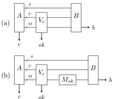
Figure 1: Games from the definition of collapse-binding commitments.

Collapse-binding commitments. To explain the definition of collapse-binding commitments, first consider a perfectly-binding commitment. That is, when an adversary A outputs a commit-mentc, there is only one possible messagemcthat Acan opencto. Hence, if the adversaryAoutputs a superposition of messages that he can open c to, that superposition will necessarily be in the state |mci. Hence, we can characterize perfectly-binding commitments by requiring: when an ad-versary outputs a superposition of messages that he can open the commitmentc to, that superpo-sition will necessarily be a single computational basis vector (i.e., no non-trivial superposition).

To express this more formally, consider the

(9)

whetherU, Mcontain matching opening information/message. More formally,Vcmeasures whether U, M is a superposition of states|u, mi such thatu is valid opening information for messagemand commitmentc. Letok = 1 if the measurement succeeds. Then we feed the registersS, U, M back to the second partB of the adversary. B outputs a classical bit b. As discussed before, a commitment is perfectly-binding iff for all adversaries A, the state of M after measuring ok = 1 is a computational basis vector.

The state of a register is a computational basis vector (or, synonymously: is in a collapsed state) iff measuring that register in the computational basis does not change that state. Consider the circuit in Figure 1 (b). Here we added a measurement Mok on

M afterVc. Mok is a complete measurement in the computational basis, but is executed

only ifok = 1. SinceMok disturbs the state of M iff that state is not a computational

basis vector, we can rephrase the definition of perfectly-binding commitments:

A commitment is perfectly-binding iff, for all computationally unlimited adversaries A, B, Pr[b= 1] is equal in Figures 1 (a) and 1 (b) wherebis the output (i.e., guess) ofB.3 Now we are ready to weaken this characterization to get a computational binding prop-erty. Basically, we require that the same holds for quantum-polynomial-time adversaries:

Definition 7 (Collapse-binding – informal) A commitment is collapse-binding iff, for all quantum-polynomial-time adversariesA, B, Pr[b= 1]in Figure 1 (a) is negligibly close toPr[b= 1] in Figure 1 (b).

In other words, with a perfectly-binding commitment, the adversary cannot produce a superposition of different messages that are contained in the commitment. But with a collapse-binding commitment, the adversary is forced to produce a statethat looks like it is not a superposition of different messages. For the purpose of computational security, this will often be as good.

We quickly explain why collapse-binding commitments work well with quantum rewinding. In the case of quantum rewinding (e.g., in the analysis of proofs of knowl-edge [Unr12]), one problem is that we might need to run an adversary until he opens a commitment c, then to measure the opened message, and then to go back to an earlier state by applying the inverse of the adversary. The problem is that measuring the opened message will disturb the state of the adversary, and thus make rewinding impossible. Except: if the opened message cannot be distinguished from being already in a collapsed state (as guaranteed by collapse-binding), then measuring the opened message does not disturb the state in a noticeable way and we can rewind. (See the discussion on arguments of knowledge below.)

Constructing collapse-binding commitments. Collapse-binding commitments are useful only if they exist. Perfectly-binding commitments are easily seen to be collapse-binding, but then we cannot have statistically hiding or short commitments. In the classical setting, we get practical computationally-binding commitments from a collision-resistant hash function H. The most obvious construction is to sendc:=H(mku) for

(10)

uniformly randomuof suitable length. We call this the “canonical commitment”. The canonical commitment is easily seen to be classical-style binding ifH is collision-resistant, and it is statistically hiding if H is a random oracle. To get rid of the random-oracle requirement, we can use a somewhat more complex constructions by Halevi and Micali [HM96] instead. Unfortunately, both the canonical commitment and the Halevi-Micali commitments are not collapse-binding ifH is merely collision-resistant. In fact, relative to a specific oracle and using a specific collision-resistant hash function, there is a total break where the adversary can unveil the commitment to any message of his chosing. To show this, we tweak the technique from [ARU14] to construct a hash function H such that the adversary can sample an image c of H together with a quantum state

|Ψi such that: Given the state|Ψi, for anym, the adversary can find a random u with H(mku) =c. But this process destroys|Ψi, so the adversary cannot find two preimages of c; the hash function is collision-resistant. But the canonical commitment, based on this H, is trivially broken. Similar constructions break the Halevi-Micali commitments. Since collision-resistance seems too weak a property in the quantum setting (at least for our purposes), we give a strengthening of collision-resistance: collapsing hash functions:

Definition 8 (Collapsing hash function – informal) An adversary is valid if he outputs a classical valuec, and a register M containing a superposition of messagesm

with H(m) = c. We call H collapsing iff no quantum-polynomial-time adversary can distinguish whether we measure M in the computational basis or not, before giving the register M back to the adversary. (This is formalized with games similar to those in Figure 1.)

We can show that collapsing hash functions are collision-resistant, and they share a number of structural properties with collision-resistant functions. E.g., injective functions are collapsing, and the composition H◦H0 of collapsing functions is collapsing.

Due to the similarity between the definition of collapsing hash functions and collapse-binding commitments, we can show that the canonical commitment and the Halevi-Micali commitments are collapse-binding if H is collapsing.

However, this leaves the question: do collapsing functions exist in the first place? We conjecture that common industrial hash function like SHA3 [NIS14] are actually collapsing (not only collision-resistant). In fact, we argue that the collapsing property should be a requirement for the design of future hash functions (in the sense that a hash function where the collapsing property is in doubt should not be selected for industry standards), since collision-resistance is not sufficient if we wish to achieve post-quantum secure cryptography. We support our conjecture that sufficiently unstructured functions are collapsing by proving that the random oracle is collapsing:

(11)

realistic modeling of hash functions [BDF+11]. As a first step, we identify a new property, “half-collision resistance”:

Definition 9 (Half-collision resistance – informal) A half-collision of H is a string x such that there exists an x0 6= x with H(x0) = H(x). A hash function H

is half-collision resistant if no adversary does the following: He outputs a half-collision with non-negligible probability. And he never outputs a non-half-collision. (The adversary may output⊥ though.)

That is, half-collision resistance says that the adversary cannot find non-injective inputs to H without sometimes accidentally outputting injective inputs. We show: if H is half-collision resistant, it is collapsing.

The proof idea is: ifH is not collapsing, the adversary can produce a superpositionM of messages m with H(m) = c and notice whether M is being measured. The latter implies that M must be a superposition of at least two messages m with H(m) = c. Hence by measuring M, the adversary gets a half-collision. Much additional work is needed to make sure that the adversary does not accidentally measure the registerM when it is not a nontrivial superposition.

(The half-collision resistance property might be useful independent of the proof that the random oracle is collapsing. When trying to construct collapsing hash functions based on other assumptions, half-collision resistance might be easier to verify since its definition consists of purely classical games.)

Next we construct a random function H∗ :X →Y with |Y|= 2₃|X|. That is, H∗ is slightly compressing. The domain of H∗ is partitioned into two sets X1, X2 with

|X1|= 2|X2|. H∗ is injective onX2, and 2-to-1 onX1. Besides those constraints, H∗ is uniformly random. We can then show thatH∗ is half-collision resistant. (Basically, this means that the adversary cannot identify the subsetX1.) Furthermore, we can show that H∗ is indistinguishable from a random functionH :X →Y. The latter fact is shown by step-wise rewriting of the definition ofH∗ until we reachH (crucially using the fact that random functions and random injections are indistinguishable [Zha15]). SinceH∗ is half-collision resistant, it is collapsing. And since H is indistinguishable fromH∗,H is collapsing.

We now know that random functions H :X →Y are collapsing if |Y|= 2₃|X|(i.e., if they are slightly compressing). However, we want that H is collapsing for arbitrary X and Y, as long as Y has superpolynomial size. For|X| ≤ |Y|,H is indistinguishable from a random injection, which in turn is collapsing. The interesting case is|X|>|Y|

(namely, whenH is compressing). In this case, we show (following an idea from [Zha15]) thatH can be written asH =fn◦ · · · ◦f1 where allfi are slightly compressing. (Some technical care is needed when |Y|/|X|is not a power of 2₃.) Since all fi are collapsing, so is H. This shows that a random functionH is collapsing, in other words, that the random oracle is collapsing (if its range has superpolynomial size).

(12)

Unruh showed that a sigma-protocol (i.e., a particular kind of three round proof system) is a quantum proof of knowledge if it has two properties: special soundness (from two interactions with the same first and different second messages one can efficiently compute a witness) and strict soundness (the first and second message of a valid interaction determine the third). In the classical setting, only special soundness is needed. In the quantum setting, strict soundness is additionally required to allow for quantum rewinding: In the proof from [Unr12], we run the malicious prover to get his response (the third message). Then we measure the response. Then we rewind the prover (by applying the inverse of the unitary transformation representing the prover). Then we run the prover again to get a second answer. Special soundness then implies that from the two responses, we get a witness. However, we need to make sure that measuring the prover’s response before rewinding does not disturb the state (too much). In [Unr12], this follows from strict soundness: strict soundness guarantees that the response is uniquely determined, and thus measuring the response does not disturb the state. To achieve strict soundness, [Unr12] lets the prover commit to all possible responses in the first message using perfectly-binding commitments.4 _{The drawback of this solution is that the} commitments cannot be statistically hiding, so we cannot get statistical zero-knowledge proofs using the method from [Unr12].

What happens if we replace the perfectly-binding commitments by collapse-binding commitments containing the response? In that case, the response will not necessarily be information-theoretically determined by the first two messages. However, the defi-nition of collapse-binding commitments guarantees that measuring that response will be indistinguishable from not measuring it. Thus, if we measure the response, the state might be disturbed, but it will be computationally indistinguishable from not being disturbed. This is enough for the proof technique from [Unr12] to go through when using collapse-binding commitments, assuming the prover is computationally limited. The resulting protocol will not be a quantum proof of knowledge, but a quantum argument of knowledge (i.e., secure only against computationally limited provers). But in contrast to [Unr12], the proof system will be statistical zero-knowledge.

To summarize: from collapse-binding commitments (or from collapsing hash functions), we get three-round statistical zero-knowledge quantum arguments of knowledge for all languages in NP (with inverse polynomial knowledge error). To the best of our knowledge, not even three-round statistical zero-knowledge quantumarguments were known before.

1.4 Related work.

Commitments. Brassard, Crépeau, Jozsa, and Langlois [BCJL93] presented an information-theoretically hiding and binding commitment scheme using quantum com-munication. However, the protocol was flawed, Mayers [May97] showed that information-theoretically hiding and binding commitments are impossible. (This is no contradiction to our results, because our commitments are not information-theoretically binding.) Dumais, Mayers, and Salvail [DMS00] and Crépeau, Légaré, and Salvail [CLS01] constructed

4

(13)

statistically hiding commitments from quantum one-way permutations/functions, respec-tively. Their protocols use quantum communication, and are sum-binding. Cr´epeau, Dumais, Mayers, and Salvail [CDMS04] generalized the sum-binding definition to string commitments and constructed an OT protocol based on that definition. (However, it is not known whether the protocol composes even sequentially.) Damg˚ard, Fehr, Lunemann, Salvail, and Schaffner [DFL+09] and Unruh [Unr10] showed a much simpler OT protocol to be secure, assuming much stronger commitment definitions in the CRS model, but achieving stronger security notions (sequential composability/UC). Ambainis, Rosmanis, and Unruh [ARU14] show that classical-style binding commitments are not necessarily even sum-binding.

Quantum random oracles. Random oracles were first explicitly considered in a quantum cryptographic context by Boneh, Dagdelen, Fischlin, Lehmann, Schaffner, and Zhandry [BDF+11] who stressed that the adversary should have superposition access to the random oracle. Zhandry [Zha15] showed that the random oracle is collision-resistant. In contrast, we show (based on his result) that the random oracle is collapsing (a stronger property).

Quantum rewinding and proof systems. Watrous [Wat09] showed how quantum rewinding can be used to prove the security of quantum zero-knowledge protocols. Unruh [Unr12] showed how a different flavor of quantum rewinding can be used for proving the security of quantum proofs of knowledge; we extend their technique to quantum arguments of knowledge. Unruh [Unr15a] constructs non-interactive computational zero-knowledge quantum arguments of knowledge in the random oracle model.

2 Definitions and basic properties

Preliminaries. For the necessary background in quantum computing, see, e.g., [NC10]. By |ii withi∈I we denote the vectors of the computational basis of the Hilbert space with dimension |I|. We also use the symbol|·i to refer to other (non-basis) vectors (e.g.,

|Ψi). And hΨ|is the conjugate transpose of |Ψi. kxk refers to the Euclidean or`2-norm. We only consider finite dimensional Hilbert spaces. We denote |+i:= √1

2|0i+ 1 √

2|1i and

|−i:= √1 2|0i −

1 √

2|1i. For a linear operatorAon a Hilbert space, we denote by A † _its

conjugate transpose. We denote byI the identity. We call an operator A on a Hilbert space a projector iff it is an orthogonal projector, i.e., a linear map withP2 =P and P =P†. By TD(ρ, ρ0) we denote the trace distance between ρand ρ0, and byF(ρ, ρ0) the fidelity.

(14)

We call an algorithm quantum-polynomial-time if it is a quantum algorithm and its runtime is bounded by a polynomial in its input length with probability 1. We call an algorithm classical-polynomial-time if it performs only classical operations and its runtime is bounded by a polynomial in its input length with probability 1. We write 1η for a bitstring (of 1’s) of lengthη. (The latter is useful for making algorithms run in polynomial-time in the length of the security parameter, e.g., A(1η) will run polynomial-time in η.)

Commitments. A commitment scheme (com,verify) consists of a quantum-polynomial-time algorithmcom and a deterministic quantum-polynomial-time algorithm

verify.5 _{(c, u)} _← _com₍₁η_{, m) returns a commitment} _c _{and the opening information} _u for the message m and security parameter η. c alone is supposed not to reveal any-thing aboutm(hiding). To open, we send (m, u) to the recipient who checks whether

verify(1η, c, m, u) = 1. Both com andverify have classical input and output. com has a well-defined message space MSPη that also depends on the security parameterη (e.g.,

{0,1}η_{). Furthermore, for technical reasons, we assume that it is possible to find triples} (c, m, u) withverify(1η, c, m, u) = 1 with probability 1 in quantum-polynomial-time inη.6

We first state some standard properties of commitments.

Definition 10 Let (com,verify) be a commitment scheme. We define:

• Perfect completeness: (com,verify) has perfect completeness iff for all m ∈ MSPη, Pr[verify(1η, c, m, u) = 1 : (c, u)←com(1η, m)] = 1.

• Computational hiding: (com,verify) is computationally hiding iff for any quantum-polynomial-timeA and any polynomial `, there is a negligible µ such that for anyη, anym0, m1 ∈MSPη with|m0|,|m1| ≤`(η), and any|Ψi,7 P0−P1

≤µ(η)

where Pi := Pr[b= 1 : (c, u)←com(1η, mi), b←A(1η,|Ψi, c)].

• Statistical hiding: Like computational hiding, except that we quantify over all A

(not just quantum-polynomial-time A).

Definition 11 (Classical-style binding) A commitment scheme is classical-style binding iff for any quantum-polynomial-time algorithm A, the following is negligible in η:

Pr[verify(1η, c, m, u) = 1∧verify(1η, c, m0, u0) = 1∧m6=m0 : (c, m, u, m0, u0)←A(1η)]

5

To be practical, those algorithms should of course be classical. We allow quantum-polynomial-time algorithms here to state our results in greater generality.

6

This technical condition is necessary, e.g., for Definition 13 below. Without this condition, it is not clear that “valid” adversaries exist at all. Note that a commitment scheme with quantum-polynomial-time com and perfect completeness will always satisfies this technical condition: to findc, m, u, simply set m:= 0 and compute (m, u)←com(1η, m).

7_|Ψi_{is the auxiliary input of}_A_{that represents knowledge of}_A_{acquired, e.g., in prior protocol runs.}

(15)

Definition 12 (Collapse-binding) For algorithmsA,B, consider the following games:

Game1 : (S, M, U, c)←A(1η), ok ←Vc(M, U), m←Mok(M), b←B(1η, S, M, U)

Game2 : (S, M, U, c)←A(1η), ok ←Vc(M, U), b←B(1η, S, M, U)

Here S, M, U are quantum registers. Vc is a measurement whether M, U contains a valid

opening, formallyVc is defined through the projector P m,u

verify(1η_,c,m,u₎₌₁|mihm| ⊗ |uihu|.

Mok is a measurement ofM in the computational basis if ok = 1, and does nothing if ok = 0 (i.e., it sets m:=⊥ and does not touch the registerM).

A commitment scheme is collapse-binding iff for any quantum-polynomial-time algo-rithmsA, B, the difference Pr[b= 1 :Game₁]−Pr[b= 1 :Game₂]

is negligible.

Instead of measuring using Vc whether the adversary outputs a correct opening informa-tion, we can quantify only over adversaries that always output correct opening information. This leads to the following equivalent definition of collapse-binding commitments. This definition is often easier to handle when proving that a given scheme is collapse-binding.

Definition 13 (Collapse-binding – variant) For algorithmsA,B, consider the fol-lowing games:

Game1 : (S, M, U, c)←A(1η), m←Mcomp(M), b←B(1η, S, M, U)

Game2 : (S, M, U, c)←A(1η), b←B(1η, S, M, U)

Here S, M, U are quantum registers. Mcomp(M) is a measurement ofM in the computa-tional basis.

We call an adversary (A, B) valid if Pr[verify(c, m, u) = 1] = 1 when running

(S, M, U, c)←A(1η) and measuring M, U in the computational basis to obtainm, u.

A commitment scheme is collapse-bindingiff for any quantum-polynomial-time valid adversary(A, B), the differencePr[b= 1 :Game₁]−Pr[b= 1 :Game₂]

is negligible.

Lemma 14 A commitment scheme (com,verify) is collapse-binding with respect to Definition 12 iff it is collapse-binding with respect to Definition 13.

Proof. To avoid confusion, we call the games from Definition 12Game1,Game2, while we call those from Definition 13 Game0₁,Game0₂. And the adversary in Definition 13 (that is used inGame0₁,Game0₂) we call (A0, B0).

First, assume that there is an adversary (A0, B0) breaking Definition 13, i.e., µ:=

|Pr[b = 1 : Game0₁]−Pr[b = 1 : Game0₂]| is non-negligible. Let (A, B) := (A0, B0). By definition of validity, the measurement Vc from Definition 12 will succeed with probability 1 in Game1 and Game2. Hence that measurement has no effect, and thus Pr[b= 1 :Game1] = Pr[b= 1 :Game0₁] and Pr[b= 1 :Game2] = Pr[b= 1 :Game0₂]. Thus

(16)

Now, consider an adversary (A, B) breaking Definition 12, i.e., ν := |Pr[b = 1 : Game1]−Pr[b= 1 :Game2]|is non-negligible. Construct (A0, B0) as follows: A0(1η) runs (S, M, U, c)←A(1η). Then it appliesok ←Vc(M, U). Ifok = 1,A0 returns (S, M, U, c).

Otherwise,A0 picks (c, m, u) with verify(1η, c, m, u) = 1,8 initializesM, U with |mi|ui, andS with |⊥i, and outputsc. (We assume that |⊥iis orthogonal to any state that A would produce.) AndB0 does the following: Ifok = 0, thenB0 outputs 0. Ifok = 1, B0 executesB.

A0 is valid by construction: If ok = 1, verify(1η, c, m, u) = 1 with probability 1 when measuring M, U as m, u, because M, U is in the image of Vc. And if ok = 0,

verify(1η, c, m, u) = 1 by choice of c, m, u. We easily see that

0 = Pr[b= 1 :Game0₁|ok = 0] = Pr[b= 1 :Game0₂|ok = 0] = 0

α:= Pr[b= 1 :Game1|ok = 0] = Pr[b= 1 :Game2|ok = 0]

β := Pr[b= 1 :Game1|ok = 1] = Pr[b= 1 :Game01|ok = 1]

γ := Pr[b= 1 :Game2|ok = 1] = Pr[b= 1 :Game02|ok = 1]

δ := Pr[ok = 1 :Game1] = Pr[ok = 1 :Game0₁] = Pr[ok = 1 :Game2] = Pr[ok = 1 :Game02]

and from this we calculate

Pr[b= 1 :Game0₁]−Pr[b= 1 :Game0₂]

=

0(1−δ) +βδ

− 0(1−δ) +γδ =

α(1−δ) +βδ

− α(1−δ) +γδ

=Pr[b= 1 :Game₁]−Pr[b= 1 :Game₂] =ν

which is non-negligible. Thus (A0, B0) breaks Definition 13.

Definition 12 guarantees that the adversary cannot distinguish whether the register M is measured or not. However, it is not immediately obvious what happens when we measure M partially (e.g., we measure just one qubit). Could it be that such a partial measurement will be noticed? We expect that this is not the case, since a partial measurement lies half-way between no measurement and a complete measurement. The following lemma confirms that intuition: If a commitment scheme is collapse-binding, then Definition 12 also holds for partial measurements. (Assuming that the partial measurement is performed in the computational basis and can be implemented by a polynomial-time circuit.)

Lemma 15 (Collapse-binding w.r.t. partial measurements) For a commitment scheme (com,verify), and for algorithms A, B, consider the following games:

Game1 : (S, M, U, c, f)←A(1η), ok ←Vc(M, U), x←M_okf (M), b←B(1η, S, M, U)

Game2 : (S, M, U, c, f)←A(1η), ok ←Vc(M, U), b←B(1η, S, M, U)

(17)

Here f is a Boolean circuit (with multiple-bit output). Vc is as in Definition 12. M_okf is

a measurement of M that returns f(m) where m is the content ofM if ok = 1, and does nothing if ok = 0(i.e., it sets m:=⊥ and does not touch the registerM). More formally, if ok = 1, Mf is the measurement defined by the projectors Px:=Pm:f(m)=x|mihm|for

allx in the range of f, and if ok = 0, Mf is defined by the single projectorP⊥:=I.

If (com,verify) is collapse-binding, then for any quantum-polynomial-time adversary

(A, B), the differencePr[b= 1 :Game₁]−Pr[b= 1 :Game₂]

is negligible.

Proof. We start with Game1. It is easy to see that Vcand M_okf commute, and thatVc is idempotent. Thus Pr[b= 1 :Game1] = Pr[b= 1 :Game3] with:

Game3 : (S, M, U, c, f)←A, ok0 ←Vc, x←M_okf 0, ok ←Vc, b←B

(We omit the inputs of the various algorithms and measurements since they are unchanged throughout the proof.) If we consider the first three operations (A, Vc, M_okf0) as a

single adversary, we can apply the collapse-binding property of com. Thus |Pr[b= 1 : Game3]−Pr[b= 1 :Game4]|=ε1 for some negligibleε1 with:

Game4 : (S, M, U, c, f)←A, ok0←Vc, x←M_okf 0, ok ←Vc, m←Mok, b←B

We can see that Vc, M_okf 0, Mok all commute. Furthermore Vc is idempotent, so we get Pr[b= 1 :Game4] = Pr[b= 1 :Game5] with:

Game5: (S, M, U, c, f)←A, ok ←Vc, m←Mok, x←M_okf , b←B

(Note that we replace M_okf 0 by M_okf .) The outcome ofM_okf is determined by the outcome

of Mok, we have Pr[b= 1 :Game5] = Pr[b= 1 :Game6] with:

Game6: (S, M, U, c, f)←A, ok ←Vc, m←Mok, b←B

Since (com,verify) is collapse-binding, we get|Pr[b= 1 :Game6]−Pr[b= 1 :Game2]|=ε2 for negligible ε2.

Thus, summarizing,|Pr[b= 1 :Game1]−Pr[b= 1 :Game2]| ≤ε1+ε2 is negligible.

Another question that naturally arises is whether collapse-binding commitments parallel compose. That is, if we commit to values m1, . . . , mn with n commitments, does this give a collapse-binding commitment onm:= (m1, . . . , mn)? Note that such a property is not obvious. For example, to the best of our knowledge, no prior definition of a quantum computational binding property in the literature is known to have this property. For collapse-binding commitments, however, the next lemma shows that the parallel composition of several commitments is still collapse-binding.

(18)

Let (comn,verifyn) be the n-fold parallel composition of (com,verify). That is, its message space is Mp. And comn(m1, . . . , mn) computes (ci, ui) ← com(mi) for i = 1, . . . , n, and returns (c, u) with c := (c1, . . . , cn) and u := (u1, . . . , un). And

verifyn((c1, . . . , cn),(m1, . . . , mn),(u1, . . . , un)) = 1iff ∀i.verify(ci, mi, ui) = 1.

Then (comn,verifyn) is collapse-binding.

Proof. By Lemma 14, to show that (comn,verifyn) is collapse-binding, we need to show that for any valid adversary Aagainst (comn_,_verifyn_),

Pr[b= 1 :Game₁]−Pr[b= 1 : Game2] is negligible, withGame1,Game₂ as follows:

Game1: (S, M, U, c)←A(1η), m←Mcomp(M), b←B(1η, S, M, U)

Game2: (S, M, U, c)←A(1η), b←B(1η, S, M, U)

Using the definition of (comn,verifyn), this is equivalent to:

Game1: (S, M1, . . . , Mn, U1, . . . , Un, c1, . . . , cn)←A(1η),

mi ←Mcomp(Mi) for i= 1, . . . , n,

b←B(1η, S, M1, . . . , Mn, U1, . . . , Un)

Game2: (S, M1, . . . , Mn, U1, . . . , Un, c1, . . . , cn)←A(1η),

b←B(1η, S, M1, . . . , Mn, U1, . . . , Un)

And the validity of Aimplies for all i that measuringMi, Ui will always returnmi, ui with verify(ci, mi, ui) = 1.

We define hybrid games for i= 0, . . . , n:

Hyb_j : (S, M1, . . . , Mn, U1, . . . , Un, c1, . . . , cn)←A(1η),

mi ←Mcomp(Mi) for i= 1, . . . , j,

b←B(1η, S, M1, . . . , Mn, U1, . . . , Un)

Note that in Hyb_j, only M1, . . . , Mj are measured. Mj+1, . . . , Mn are untouched. We immediately have

Pr[b= 1 :Game1] = Pr[b= 1 :Hybn], Pr[b= 1 :Game2] = Pr[b= 1 :Hyb0]. (1)

We define a new adversary (A0, B0) for (com,verify) as follows: A0(1η) picksj← {$ 1, . . . , n}. Then he executes (S, M1, . . . , Mn, U1, . . . , Un, c1, . . . , cn) ←A(1η). He measuresmi ← Mcomp(Mi) for i= 1, . . . , j−1, and then sets

S0:= (j, S, M1, . . . , Mj−1, Mj+1, . . . , Mn, U1, . . . , Uj−1, Uj+1, . . . , Un)

(19)

As mentioned above, since A is valid for each i, measuring Mi, Ui returns mi, ui withverify(1η, ci, mi, ui) = 1. Hence measuringM, U as output by A0 returnsm, uwith

verify(1η, c, m, u) = 1. Thus A0 is valid for (com,verify). Thus Pr[b= 1 :Game0₁]−Pr[b= 1 :Game0₂]

is negligible whereGame0₁,Game0₂ are as follows:

Game0₁: (S0, M, U, c)←A(1η), m←Mcomp(M), b←B(1η, S0, M, U)

Game0₂: (S0, M, U, c)←A(1η), b←B(1η, S0, M, U)

For any fixed choice ofj,Game0₁ is the same as Hyb_j, andGame0₂ is the same asHyb_j₋₁. Thus

Pr[b= 1 :Game0₁] = n X

j=1 1

nPr[b= 1 :Hybj],

Pr[b= 1 :Game0₁] = n X

j=1 1

nPr[b= 1 :Hybj−1].

(2)

Hence

Pr[b= 1 :Game0₁]−Pr[b= 1 :Game0₂]

(2)

= 1_nPr[b= 1 :Hyb_n]−Pr[b= 1 :Hyb₀]

(1)

= 1_nPr[b= 1 :Game1]−Pr[b= 1 :Game2]

(3)

We showed above that the lhs of (3) is negligible. Thus the rhs of (3) is negligible, too. Sincen is polynomially-bounded in η, this implies thatPr[b= 1 :Game1]−Pr[b= 1 : Game2] is negligible as well. As stated in the beginning of this proof, this implies that (comn,verifyn) is collapse-binding.

3 Commitments from collision-resistant hash functions

In the following, we will often refer to hash functions. We will always assume that a hash function depends implicitly on the security parameter (in particular, the size of the range can depend on the security parameter). We also assume that the hash function is quantum-polynomial-time computable (inη and the input length).9 Besides that, we do not assume any further properties such as collision-resistance unless explicitly mentioned.

Definition 17 (Canonical commitment scheme) Given a hash function H and a parameter `u=`u(η), the canonical commitment scheme for H is:

• Message spaceMSPη :={0,1}∗.

• comcan(m): Pick u

$

← {0,1}`u_{. Compute} _c_:=_H(m_k_u)_{. Return} _{(c, u)}_.

• verify_can(c, m, u): Return 1 iff H(mku) =c.

9_{When working in the random oracle model: Quantum-polynomial-time computable given access to}

(20)

It is immediate to see that this scheme is classical-style binding if H is collision-resistant. However, in general it will not be hiding; for example, H(mku) could leak the first bit of m. However, it is hiding ifH is a random oracle:

Lemma 18 Fix `u≥0 and assume that|Y| ≤2`u/8. For a random oracle H :X→Y,

the canonical commitment is statistically hiding.

Proof. This lemma was proven in [Pas04, Lemma 9]. The statement of the lemma there additionally assumes that the message space of the canonical commitment is also{0,1}`u

(i.e., equal to the space of the randomnessu). However, this is never used in the proof. Furthermore, the lemma there assumes that|Y|= 2`u/8_{, but the adaption to the case}

|Y| ≤2`u/8 _{is straightforward.}

When using a hash function in the standard model, we can use the following commitment scheme instead:

Definition 19 (Bounded-length Halevi-Micali commitment [HM96]) Fix inte-gers`=`(η),n=n(η). LetL:= 4`+ 2n+ 4. LetH :{0,1}L_{→ {}_0,₁_}`_{be a hash function.}

LetF =F(η)be a family of universal hash functionsf :{0,1}L_{→ {}_0,₁_}n_{. We define the} bounded-length Halevi-Micali commitment (comHMb,verifyHMb) with MSPη = {0,1}n as:

• comHMb(m): Pick f ∈ F and u∈ {0,1}L uniformly at random, conditioned on

f(u) =m. Compute h:=H(u). Letc:= (h, f). Return (c, u).

• verify_HMb(c, m, u) with c= (h, f): Check whether f(u) =mand h=H(u). If so, return1.

Definition 20 (Unbounded Halevi-Micali commitment [HM96]) Fix an integer

`=`(η). Let H :{0,1}∗ _{→ {}_0,₁_}` _{be a hash function. Let} _L_{:= 6`}_{+ 4}_{. Let} _F _{be a family}

of universal hash functionsf :{0,1}L_{→ {}_0,₁_}`_{. We define the} _{unbounded Halevi-Micali} commitment (comHMu,verifyHMu) as:

• comHMu(m): Pick f ∈ F and u ∈ {0,1}L uniformly at random, conditioned on

f(u) =H(m). Computeh:=H(u). Let c:= (h, f). Return (c, u).

• verify_HMu(c, m, u) withc= (h, f): Check whetherf(u) =H(m) and h=H(u). If so, return 1.

Theorem 21 (Security of Halevi-Micali [HM96]) If`is superlogarithmic, then the Halevi-Micali commitment and the bounded-length Halevi-Micali commitment are sta-tistically hiding. IfH is collision-resistant, then the Halevi-Micali commitment and the bounded-length Halevi-Micali commitment are classical-stylebinding.

Note that [HM96] did not prove the classical-style binding property against quantum

(21)

The following theorem shows that collision-resistance does not seem to be enough to make the above constructions secure in the quantum setting, i.e., classical-style binding is all we get.

Theorem 22 There is an oracleO relative to which there exists a collision-resistant10 hash function H such that the canonical commitment scheme and both Halevi-Micali commitment schemes using H admit the following attack:

There is a quantum-polynomial-time adversaryAO that outputs a commitmentc, then expects a bitb, and then outputs with overwhelming probability a pair (m, u) such that verify(c, m, u) = 1 and the first bit of m is b.

Clearly, a commitment with that property should not be considered secure. This shows that collision-resistance is too weak a property for constructing commitments in the quantum setting, at least when using standard constructions.

Proof. [ARU14, Definition 6] defines a specific oracle O_all (more precisely, a probability distribution on oracles). We repeat only the parts of the construction that are relevant for our proof: Let X :={0,1}`1 _and_Y _:=_{_0,₁_}`2 _{for some arbitrary polynomially-bounded}

superlogarithmic `1, `2. For each y ∈ Y, let Sy ⊆ X be a uniformly random subset of a certain size k. Let OV be an oracle that tests membership in Sy, more precisely O_V(y, x) = 1 iff x∈Sy. (OV may be queried in superposition.) Finally,Oall is defined

to be an oracle consisting ofO_V and several other oracles (some of them implementing unitary transformations).

We use the following important facts about O_all:

Fact 1 (Hardness of two values) LetAbe an algorithm making a polynomial number of oracle queries. Then Pr[x6=x0 ∧ x, x0 ∈Sy : (y, x)←AOall(1η)] is negligible.

This fact is a reformulation of [ARU14, Corollary 7 (i)].

Fact 2 (Searching one value) There is a pair (E1, E2) of quantum-polynomial-time

oracle algorithms such that:

• EOall

1 (1η) outputs y∈Y and a quantum state |Ψ(y)i.

• Given a Boolean circuit P with |{x ∈ Sy : P(x) = 1}| ≥ |Sy|/3, EOall

2 (1η, y,|Ψ(y)i, P) outputs x ∈ Sy with P(x) = 1 with overwhelming

proba-bility.

This is a special case of [ARU14, Theorem 5].11

Informally, Fact 2 tells us that if we choose y ∈ Y ourselves, we get a quantum trapdoor |Ψ(y)i that allows us to searchone value x∈Sy satisfying a predicate of our

10

H is collision-resistant iff for any quantum-polynomial-timeA, Pr[x6=x0∧H(x) =H(x0) : (x, x0)← A(1η_{)] is negligible.}

11

We have fixedδmin:= 1/3 andnto be the security parameter, and we have removed the argument

(22)

choice, as long as this predicate is satisfied 1₃ of the time. (But note: we cannot get two such x in the sameSy, as this would violate Fact 1.)

Let h2 :{0,1}∗ → {0,1}` (for some arbitrary polynomially-bounded superlogarithmic `) be uniformly random. We can then define the oracleO to be the oracle containing

O_all and h2. (I.e.,O gives access toO_all and an additional random oracle.) Note that sinceh2 and Oall are independent, Fact 1 still applies when Ais given access to O.

We now construct a hash function H : {0,1}∗ → {0,1}`_{. For} _x _∈_X_, _y _∈ _Y _with OV(y, x) = 1, let h1(xky) := 0ky and leth1(z) := 1kzeverywhere else. Let H :=h2◦h1.

Claim 1 (Collision-resistance of H) H is collision-resistant (relative toO).

To show this, we show thath1 and h2 are collision-resistant relative toO. This then shows thatH =h2◦h1 is collision-resistant relative toO. Any collision of h1 must be of the formh1(xky) =h1(x0ky0) with xky 6=x0ky0 and OV(y0, x0) =OV(y, x) = 1 since h1 is injective everywhere else. By definition of h1, this implies that 0ky = 0ky0, thus y=y0 and x6=x0. And thenOV(y0, x0) =OV(y, x) = 1 implies by definition ofOV that x, x0 ∈Sy. By Fact 1, a polynomial-time adversary with oracle access to O finds such x, x0, y only with negligible probability. This shows that h1 is collision-resistant relative toO.

By [Zha15, Theorem 3.1], h2 is collision-resistant (given oracle access to h2).12 Since O_all is chosen independently of h2, it can be simulated with no extra queries to h2. I.e., an adversary breaking collision resistance of h2 using O = (Oall, h2) can

be transformed into one breaking collision resistance of h2 using h2. Hence h2 is also collision-resistant given oracle access toO.

Thus h1, h2 are collision-resistant relative to O, and thus H =h2◦h1 is collision-resistant relative toO.

Attack on the canonical commitment scheme. Let `m be some arbitrary message length, and`u the length of the opening information (see Definition 17). For this attack, we assume that the length parameters `1, `2 in the construction of O_all have been chosen such that `m+`u=`1+`2. (This is always possible, since`1, `2 are only required to be superlogarithmic.) The adversaryA does the following:

• LetE1, E2 be the algorithms from Fact 2.

• (y,|Ψ(y)i)←EOall

1 (1η). Letc:=h2(0ky) and send cas the commitment.

• Upon input b, choose P such that P(x) := 1 iff the first bit of x is b. Run x←EOall

2 (1η, y,|Ψ(y)i, P). Splitxky as mku:=xky with |m|=`m,|u|=`u and send (m, u). (Note: the lengths ofm, u do not necessarily match the lengths ofx, y, but their combined length does since`1+`2=`m+`u.)

12

Strictly speaking, [Zha15, Theorem 3.1] only applies to random oracles with finite but arbitrary large domain, not toh2 which has domain{0,1}∗. However, if an adversary finds a collision inh2 with

non-negligible probabilityµ, then there must be a length`∗ such that the adversary finds a collision of length at most`∗with probability at leastµ/2. Thus an adversary breaking collision-resistance ofh2

(23)

Since Sy ⊆ Y is a random set of (superpolynomial) cardinality k, we have that the fraction of Sy having leading bit b (i.e., satisfying P) is at least 1₃ with overwhelming probability. Thusx as returned byE2 satisfies, by Fact 2, with overwhelming probability x ∈ Sy and P(x) = 1. From P(x) = 1 it follows that the first bit of m is b as required. And x ∈ Sy implies OV(y, x) = 1 which implies h1(xky) = 0ky. Hence H(mku) =h2(h1(xky)) =h2(0ky) =c. Thus verifycan(c, m, u) = 1. This shows that the

attack on the canonical commitment is successful with overwhelming probability.

Attack on the bounded-length Halevi-Micali commitment. Let n be the mes-sage length, and `, L as in Definition 19. For this attack, we assume that the length parameters `1, `2 have been chosen such that `1+`2 =L. (This is always possible, since `1, `2 are only required to be superlogarithmic.) The adversary Adoes the following:

• (y,|Ψ(y)i)←EOall

1 (1η). Pickf ∈F (the family of universal hash functions). Let h:=h2(0ky) and letc:= (h, f) and send cas the commitment.

• Upon input b, choose P such that P(x) := 1 iff the first bit of f(x) is b. Run x←EOall

2 (1η, y,|Ψ(y)i, P). Letu:=x and m:=f(u) and send (m, u).

Similarly as for the attack on the canonical commitment, we get that Agets with over-whelming probability an x∈Sy withP(x) = 1 which then impliesverifyHMb(c, m, u) = 1.

Attack on the unbounded Halevi-Micali commitment. We describe the attack on the unbounded Halevi-Micali commitment. Let `m be a superpolynomial message length, and Lthe length of the opening information (see Definition 20). For this attack, we assume that the length parameters `1, `2 have been chosen such that `1+`2 = `m. (This is always possible, since `1, `2 are only required to be superlogarithmic.) The

adversaryA does the following:

• (y,|Ψ(y)i) ←EOall

1 (1η). Pick f ∈ F and u ∈ {0,1}L such that f(u) = h2(0ky). Compute h:=H(u). Let c:= (h, f) and send cas the commitment.

• Upon inputb, letP(x) := 1 iff the first bit ofxisb. Runx←EOall

2 (1η, y,|Ψ(y)i, P). Letm:=xky. Send (m, u).

Similarly as for the attack on the canonical commitment, we get that Agets with over-whelming probability anx∈Sy withP(x) = 1 which then impliesverifyHMu(c, m, u) = 1.

4 Collapsing hash functions

(24)

The definition of collapsing hash functions is similar to that of collapsing commitments (Definition 13).

Definition 23 (Collapsing) For a function H and algorithms A, B, consider the following games:

Game1 : (S, M, c)←A(1η), m←Mcomp(M), b←B(1η, S, M)

Game2 : (S, M, c)←A(1η), b←B(1η, S, M)

HereS, M are quantum registers. Mcomp(M)is a measurement ofM in the computational basis.

We call an adversary(A, B) validifPr[H(m) =c] = 1when we run (S, M, c)←A(1η)

and measure M in the computational basis as m.

A function H is collapsing iff for any quantum-polynomial-time valid adversary

(A, B), the difference adv :=Pr[b= 1 :Game1]−Pr[b= 1 :Game2]

is negligible. (We

call adv the advantage.)

Notice that the definition of collapsing hash functions is inherently quantum, even though the object we consider (the hash functionH) is classical. We know of no classical analogue to collapsing hash functions. However, a collapsing hash function will necessarily be collision-resistant, see Lemma 25 below.

We proceed to give a number of useful properties of collapsing hash functions.

Lemma 24 An injective functionH is collapsing with advantage 0.

Proof. Consider an adversary (A, B) against Definition 23. Since (A, B) is valid, by definition we have thatm←Mcomp(M) in Game1 returns m withH(m) =c. Since H is injective, this means there is only one suchm. ThusM is in state |mi before applying m←Mcomp(M), and the measurementMcomp(M) does not change the state ofM. Thus

Pr[b= 1 :Game1] = Pr[b= 1 :Game2].

Lemma 25 A collapsing hash function is collision resistant.

Proof. Assume the hash functionH is not collision resistant. Then there is a quantum adversary C that outputs a collision (m, m0) with H(x) = H(x0) with non-negligible probability µ.

We construct a quantum-polynomial-time adversary (A, B) for Definition 23. Let Abe the following quantum algorithm: It runs C to get a collision (m, m0). If (m, m0) is a collision, it stores m, m0 in the register S, and initializesM with |Ψm,m0i:=

1 √

2|mi+ 1 √

2|m

0_i_{. It sets}_c_:=_{H(m) =}_H(m0_{) and returns (S, M, c). If (m, m}0_{) is not a}

collision,A stores⊥in the registerS, initializes M with|0i, sets c:=H(0), and returns (S, M, c).

The algorithm Bretrieves m, m0 fromS. IfS contains ⊥instead, Breturns b:= 0. OtherwiseBmeasures whetherM contains|Ψm,m0i, i.e.,BmeasuresMwith the projector

(25)

By construction, (A, B) is valid.

In Game2, with probability 1−µ,B finds S to contain ⊥ and returns b = 0. If S contains a collisionm, m0, then by construction of A,M contains|Ψm,m0i, soB outputs

b= 1 with probability 1 in this case. Hence Pr[b= 1 :Game2] =µ.

In Game1, with probability 1−µ, B finds S to contain ⊥ and returns b = 0. If S contains a collisionm, m0, then by construction the state of M before Mcomp(M) is

|Ψm,m0i, hence after that measurement it is |mi or|m0i (each with probability 1

2). In each case, the measurement performed byB (projector |Ψm,m0ihΨ_m,m0|) succeeds with

probability 1₂. Thus, ifS contains a collision, B returns b= 1 with probability 1₂. Hence Pr[b= 1 :Game1] =µ/2.

Hence Pr[b= 1 :Game1]−Pr[b= 1 :Game2] = µ

2 is non-negligible, in contradiction

to the assumption thatH is collapsing.

Definition 23 guarantees that the adversary cannot distinguish whether the registerM is measured or not. Like in the case of commitments (cf. the discussion before Lemma 15) we can ask what happens when a partial measurement is performed. Analogous to Lemma 15 we get that a partial measurement cannot be noticed, either:

Lemma 26 (Collapsing w.r.t. partial measurements) For a functionH and algo-rithmsA, B, consider the following games:

Game0₁ : (S, M, c, f)←A(1η), x←Mf(M), b←B(1η, S, M)

Game2 : (S, M, c, f)←A(1η), b←B(1η, S, M)

Heref is a Boolean circuit (with multiple-bit output).13 And S, M are quantum registers.

Mf(M)measuresf(m)wheremis the content ofM in the computational basis. Formally,

Mf(M) is the measurement defined by the projectors Px :=Pm:f(m)=x|mihm| for all x

in the range of f.

If H is collapsing, then for any quantum-polynomial-time valid adversary(A, B), the differencePr[b= 1 :Game0₁]−Pr[b= 1 :Game₂]

is negligible.

Proof. The proof is analogous to that of Lemma 15. (The proof actually becomes a bit simpler, because all occurrences of and arguments relating to Vc may be omitted.)

Lemma 27 If a valid adversary (A, B) breaks the collapsing property of g ◦f with advantage ε, then there are valid adversaries (A0, B0) and (A00, B00) with advantages ε0, ε00

againstg, f, respectively, such thatε≤ε0+ε00.

(A0, B0)and (A00, B00)each perform only two additional evaluations of f in comparison to(A, B). (And one additional measurement in the computational basis. But no additional evaluations ofg.)

(26)

Proof. Consider the following circuits: A B A B A B c b /M

/S _A _B

A M B

A B c b /M /S / (4)

HereMrepresents a measurement in the computational basis. (Discarding the outcome.) By definition of ε, we have

ε=

Pr[b= 1 : lhs of (4)]−Pr[b= 1 : rhs of (4)] .

Let Uf :|xi|yi 7→ |xi|y⊕f(x)i. Since Uf is self-inverse, introducing two consecutive applications of Uf into the lhs of (4) does not change the outcome probability. That is, with

A B

A Uf Uf B

Uf Uf

A B

Uf Uf

c b /M / S / / /M 0

|0i/ /

A0 B0

(5)

we have

Pr[b= 1 : lhs of (4)] = Pr[b= 1 : (5)].

The dashed boxes in (5) define a new adversary (A0, B0) againstg. The top two wires leavingA0 contain the state ofA0, while the bottom wire M0 contains the superposition of hashed values. SinceA is valid for g◦f, M contains a superposition of valuesm with g◦f(m) =c. (By this we mean formally that the projectorP

m,u:g◦f(m)=c|mihm|applied to M passes with probability 1.) Hence M0 contains a superposition of valuesm0 =f(m) withg(m0) =c. ThusA0 is valid forg. Letε0 be the advantage of A0 againstg. That is, we have

ε0=Pr[b= 1 : (5)]−Pr[b= 1 : (6)]

with the following circuit (6):

A B

A Uf Uf B

Uf M Uf

A B

Uf Uf

c b / M / S / / /M 0 /

|0i/ /

A0 B0

(27)

We now change the circuit slightly: Instead of discarding the outcome of the measurement

M, we assign it to the classical variablec00.

A B

A Uf Uf B

Uf M Uf

A B

Uf Uf

c

c00

b /M

/S

/

/ M

/M

0

/

|0i/ /

A00 B00

(7)

Obviously, not discardingc00 does not change the distribution of b, hence

Pr[b= 1 : (6)] = Pr[b= 1 : (7)].

The dotted lines in (7) define an adversary (A00, B00) against f. The wires S and M0 together form the state of (A00, B00), and the middle wire M is supposed to contain the hashed values. If M contains the valuem, then M0 contains f(m) and c00 will be f(m). Thus, if we measure a particular value c00, then M contains a superposition of values mwith f(m) =c00. Thus, (A00, B00) is valid for f. Letε00 be the advantage of (A00, B00) againstf. Then we have

ε00=Pr[b= 1 : (7)]−Pr[b= 1 : (8)]

with the following circuit (8):

A B

A Uf M Uf B

Uf M Uf

A B

Uf Uf

c

c00

b /M

/S

/ / M

/M

0

/

|0i/ /

A00 B00

(8)

The subcircuit consisting of the two Uf and the two measurementsMis easily seen to be equivalent to a measurementMon the M wire (since we do not use the outcomec00). Thus

Pr[b= 1 : (8)] = Pr[b= 1 : rhs of (4)].

Collecting all inequalities, we get:

ε=Pr[b= 1 : lhs of (4)]−Pr[b= 1 : rhs of (4)]

≤ε0+ε00.

Corollary 28 If f and g are collapsing, so is g◦f.

(28)

5 Commitments from collapsing hash functions

In Section 3 we saw that collision-resistant hash functions are not sufficient for several standard constructions of commitment schemes. We will now show that those same constructions are secure in the quantum setting when using collapsing hash functions instead.

The following lemma (and its Corollary 30 below) allows us to extend the message space of a collapsing commitment by hashing the message with a collapsing hash function. Besides being useful in its own right, we need it in the analysis of the unbounded Halevi-Micali commitment. The proof of the lemma is similar to that of Corollary 28.

Lemma 29 Letf be a hash function. Let (com,verify) be a commitment scheme. Let comf(1η, m) := com(f(m)) and verifyf(1η, c, m, u) = verify(1η, c, f(m), u). If a valid

adversary (A, B) breaks the collapse binding property of (comf,verifyf) with advantageε

(with respect to Definition 13), then there are valid adversaries(A0, B0) and (A00, B00) with advantages ε0, ε00 against the collapse binding property of (com,verify) and the collapsing property of f, respectively, such that ε≤ε0+ε00.

(A0, B0)and (A00, B00)each perform only two additional evaluations of f in comparison to(A, B). (And one additional measurement in the computational basis. But no additional evaluations of com or verify.)

Proof. Consider the following circuits:

A B

c

b /M

/S /U

A B

A M B

A B

c

b /M

/S /U

/ (9)

HereMrepresents a measurement in the computational basis. (Discarding the outcome.) By definition of ε, we have

ε=

Pr[b= 1 : lhs of (9)]−Pr[b= 1 : rhs of (9)] .

Let Uf :|xi|yi 7→ |xi|y⊕f(x)i. Since Uf is self-inverse, introducing two consecutive applications of Uf into the lhs of (9) does not change the outcome probability. That is, with

A B

A Uf Uf B

Uf Uf

A B

Uf Uf

c

b /M

/ S / U

/ /

/M

0

|0i/ /

A0 B0

Computationally binding quantum commitments

Computationally binding quantum commitments

Contents

1

Introduction

2

Definitions and basic properties

3

Commitments from collision-resistant hash functions

4

Collapsing hash functions

5

Commitments from collapsing hash functions