Target Recognition Method for Support Vector Machine on Stomach
Tumor Imaging
Gong Chen1, *, Ye-Rong Zhang1, and Fang-Fang Wang1, 2
Abstract—In stomach tumor imaging, traditional time domain algorithm, i.e., back projection (BP) algorithm, and traditional frequency domain algorithm, i.e., frequency wave number migration (F-K) algorithm, can locate tumor target accurately. However, BP and F-K algorithms perform poorly in identifying tumor sizes and shapes. The algorithms must consider the influence of various tissues in the human body: the attenuation of the signal strength of electromagnetic waves, the decrease in speed and the refraction due to the different permittivities between different organs of the body. These factors will eventually lead to image offset and even generate a virtual image. It is effective to refrain the displacement of image with modifying the time element of the imaging algorithm by iteration. This paper proposes a method based on combination of support vector machine (SVM) with BP and F-K algorithms to solve problems in recognizing tumor shape. The method uses field strength obtained by BP and F-K algorithms as input in SVM to establish the SVM model. Based on BP algorithm, recognition method for SVM includes the following characteristics: short prediction time of SVM and good virtual elimination effect. However, the algorithm requires long periods and possibly misses tumor targets. Except the same characteristics as BP algorithm: short prediction time of SVM and good virtual elimination effect, F-K algorithm also works more efficiently, does not miss any tumor targets, and conforms more with requirements of real-time imaging. When the data are contaminated by noises, the tumor shape in the stomach can still be suitably predicted, which demonstrates the robustness of the method.
1. INTRODUCTION
Electromagnetic inverse scattering retrieves spatial positions, sizes, shapes, and electromagnetic properties of targets in scattering field. This theory is widely used in medical imaging, target recognition, earthquake relief, and city construction [1–4].
Gastrointestinal (GI) tract is a hollow and muscular conduit which is one from the mouth to the anus. It has been reported that GI-tract-related cancers such as gastric cancers, esophagus and colon cancers have been ranked the third, fourth, and fifth causes of male’s cancer deaths, respectively while they have been ranked the fourth, fifth, and sixth causes of female’s cancer deaths, respectively, in Hong Kong in 2014 [2]. Tumors in gastrointestinal (GI) tract greatly threaten human’s health.
In order to diagnose GI tract cancers, a novel technique of endoscopy, wireless capsule endoscopy (WCE) was introduced in 2000 [5]. It consists of a short-focal-length camera, light source and radio transmitter. After it is swallowed by a patient, the capsule moves, relies on the self peristalsis of the human GI tract, through esophagus, stomach, and finally drains out of the body. The camera takes photos of the GI tract producing thousands of images in each examination. It would be time consuming for physicians to spend two or more hours to review all the images, which also increased
Received 9 May 2017, Accepted 4 August 2017, Scheduled 11 August 2017 * Corresponding author: Gong Chen ([email protected]).
chances of mistakes and misdiagnosis while the physicians focused on a small part of the field for a long time. In [6], Hu et al. proposed a new compact and panoramic image representation for WCE images. Recently, Li and Meng study a computerized tumor detection system for WCE images, which exploits textural features and support vector machine (SVM) based feature selection [7–10]. Hwang and Celebi [11] introduced an unsupervised detection of polyps in WCE images based on Gabor texture features and K-means clustering. Their works have achieved detection of bleeding and ulcer in WCE images, but not get real-time imaging. Therefore, a new kind of capsule endoscopy with through-body radar is utilized in this paper for the first time.
In stomach cancer imaging problems, electromagnetic environment poses complexity because of the unclear corresponding relationship between received and tumor signals. Tumor target is close to near field of antenna. Thus, a model must be simulated first. In this study, finite difference time domain (FDTD) method [12] is used to simulate the stomach model. Simulation experiments determine different shapes, positions and quantities of tumors.
This study uses two imaging algorithms: back projection (BP) [13, 14] and frequency wave number migration (F-K) algorithms [15–17]. BP algorithm represents a typical time domain algorithm. First, propagation delay of signal is calculated. Then, calculation results are coherently super positioned. The method is simple but requires longer calculation time. F-K algorithm acts as a typical algorithm in frequency domain, which is based on wave equation. The basic principle is to map a depth migration date into time domain. This method is widely used in fields of profile detection and seismology. Benefits of F-K algorithm include short time consumption and high resolution.
Only time or frequency domain algorithm can determine the positions of tumors. Information on tumor sizes and shapes remains lacking. When multiple tumors are detected, tumors interfere with each other, which results in virtual scenes, leading to misjudgment by the doctor.
This study proposes a method based on combination of support vector machine (SVM) [18–22] with BP and F-K algorithms. BP and F-K algorithms are used to obtain characteristic data of SVM method. SVM method is used to recognize shapes and sizes of tumors and to improve resolution and accuracy of imaging results. This method is also utilized to establish statistical learning theory in Vapnik-Chervonenkis dimension and structural risk minimization theories [23–26]. SVM features a two-convex quadratic programming problem. Thus, SVM can obtain global optimal solution and prevent local optimal solution by neural networks. SVM also possesses a regularization function that prevents regularization of electromagnetic inverse scattering problem.
First, this study establishes a simple stomach model. Second, a physical model is established to simulate the actual propagation path of electromagnetic wave in human body. Then FDTD method is used to simulate this model, and radar signal is recorded at each sampling location. Scattering signals of tumor targets are obtained by background subtraction. Third, BP and F-K algorithms are used to calculate intensity value at each grid of imaging area. These field values are used as characteristic data of SVM method. Feature data and default category labels correspond to input and output of SVM, respectively. When tumors present a positive signal, the label is 1. When healthy cells exhibit a negative signal, the label is 0. Thus, SVM model is established. Finally, SVM model is used to predict imaging areas and to obtain accurate information on tumor targets with different shapes, positions and quantities [27].
Simulation results show that the method based on combination of SVM with BP and F-K algorithms not only locates tumor target accurately but also identifies tumor shape and size. SVM combined with F-K algorithm presents better recognition ability than the SVM combined with BP algorithm and requires shorter computation time. Introduction of SVM method does not play an important role in shortening imaging time. The SVM method mainly detects shape and size of tumor targets.
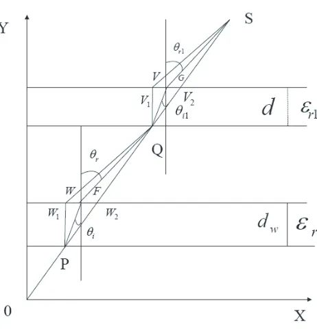
Figure 1. Refraction model.
As shown in Figure 1, the thickness of the stomach is dw, and relative dielectric constant is εr. The thickness of the abdominal muscles is d, and relative dielectric constant is εr1. In rectangular
coordinatesX-0-Y, the position of the capsule emission source is the coordinate origin, and the position of the receiving antenna is S(sx, sy). The intersection of the electromagnetic wave and the stomach is
P(px, py), and the refracted point is W(wx, wy). The coordinates of F are F(fx, fy), fx = qx−wx,
fy =qy−wy. The intersection of electromagnetic waves with the abdominal cavity is Q(qx, qy), and the refracted point isV(vx, vy). The coordinates of Gis (gx, gy),gx=sx−vx,gy =sy−vy.
The propagation path of electromagnetic wave in the stomach is calculated by the iteration method. Two extreme cases are considered: assuming that the stomach wall is air, the relative dielectric constant isεr= 1. Then there is no refraction in the electromagnetic wave, and its propagation path is straight
OPQ. The intersection of the electromagnetic wave and the stomach is W2(w2x, py +dw). It is also
assumed that the relative dielectric constant of the gastric wall is infinite. The propagation path of electromagnetic wave is approximately perpendicular to the stomach wall. The propagation path is OP W1Q, and the intersection point is W1(w1x, py +dw). Since the electromagnetic wave has to
satisfy the law of refraction on the surface of two kinds of dielectric decomposition, it can be seen that
w1 < w < w2. The geometric relationship between the incident angle and the refraction angle is as
follows:
sin(θi) = wx−px (wx−px)2+ (w
y−py)2
(1)
sin(θr) = fx
f2 x +fy2
(2)
k = sin(θi)
sin(θr) (3)
wherefx =qx−wx,fy =qy−wy,k is the refractive index,θi the incident angle, and θr the refraction angle.
The actual refractive indexW(wx, wy) is obtained by iterative method:
(a) Let the initial value of wx be the midpoint w0 of the interval (wx1, wx2), and k is obtained by
(b) k is compared with the relative dielectric constant of gastric wall tissue εr. If k < εr, take the midpoint of the interval (wx1, w0), and ifk > εr, take the midpoint of the interval (w0, wx2).
(c) Repeat steps (a) and (b) until k = εr, then the iteration stops. Finally, the refraction point
W(wx, wy) is obtained.
Similarly, the refractive index of the electromagnetic wave in the abdominal musclesεr1can be calculated
in the manner described above.
The propagation distance of electromagnetic wave in the gastric wall is l1, and the propagation
distance in non human tissues isl2+l3+l4. The propagation distance in the abdominal muscles is l5.
Then the propagation distance of electromagnetic wave is:
l = l1
v +
l2+l3+l4
c +
l5 v
= √
εrl1
c +
l2+l3+l4
c +
√
εr1l5 c
= √
εrl1+√εr1l5+l2+l3+l4 c
= deff
c (4)
wheredeff is the effective propagation distance of electromagnetic wave, cthe speed of light in vacuum, v the speed at which electromagnetic waves travel through the stomach wall and abdominal muscles,
εr the relative dielectric constant of the gastric wall, andεr1 the relative permittivity of the abdominal
cavity.
3. DESCRIPTION OF THE PROBLEM
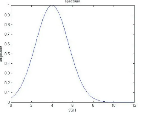
Figure 2 displays the stomach model. The model measures 20 cm in length and 12.5 cm in width in abdominal cavity. Relative dielectric constant and electrical conductivity of abdominal cavity are 36 and 7, respectively. A circular tumor model with diameter of 1 cm at coordinate site (0 cm, 4 cm) is derived. Relative dielectric constant of tumor is 50, and electrical conductivity equals 4. Signal source is (0 cm, 0 cm) in the coordinate system. Receiving antenna is placed close to outer side of the abdomen. A receiving antenna is arranged in X direction every 0.5 cm. Aperture length spans 22 cm, and the number of antennas equals 45. Transmit signal corresponds to a sine-modulated Gauss pulse with center frequency of 4 GHz and width of 0.6 ns. Figures 3 and 4 show frequency and time domain waveforms of the signal, respectively. Received signal is labeled as e(x, z = 0, t). X and Z represent abscissa and ordinate of sampled data, respectively. X andZ change alongX andZ axes, respectively, and amplitude of variation measures 0.005 m, with Δx= 0.005 m and Δz= 0.005 m. Space interval of FDTD isdx =dy = 0.5 mm, and time interval isdt= 19.25×10⁻¹². Calculation area is surrounded by perfectly matched layer-absorbing boundary.
Figure 3. Frequency domain waveform of transmitted signal.
0 0.1 0.2 0.3 0.4 0.5 0.6 0.7 0.8 0.9 1
-1 -0.8 -0.6 -0.4 -0.2 0 0.2 0.4 0.6 0.8 1
Guass function
t/ns
E(
t)
Figure 4. Time domain waveform of transmitted signal.
Regardless of whether BP or F-K algorithm is used for stomach tumor imaging, only the scattering signals of tumor must be obtained. Background signals, including reflection, refraction wave, scattering and direct signals, should be filtered to eliminate influence of human body on imaging results [28–30]. This study uses background subtraction to extract tumor signals. Steps of background subtraction are as follows:
(i) The model with tumor is simulated by FDTD method, and all radar signals on receiving antenna are recorded.
(ii) Simulation is conducted again after removing the tumor from Step 1 model without changing the other parameters. All radar signals on receiving antenna are recorded again.
(iii) Scattering signal of tumor is obtained after subtraction of radar signal in Step 1 from radar signal in Step 2.
4. BP F-K ALGORITHMS
In stomach tumor imaging, gastric model comprises tumor and healthy cells. Owing to large difference in electrical parameters (including dielectric constant and conductivity) between tumor and healthy cells, the model can be regarded as two classes: tumor cells represent the positive class, and healthy cells correspond to negative class. SVM performs well in binary classification. Simulation data are obtained by FDTD method. In this method, imaging area is divided into fixed meshes. Each mesh corresponds to a cancer or healthy cell and is labeled as positive or negative one, respectively. Negative class is marked as 0, and positive class is marked as 1. Input and output of SVM exhibit a one-to-one mapping relationship. Therefore, characteristic value of each mesh must be determined. Flow of BP algorithm is as follows:
(i) Imaging area is divided into a certain mesh intervals.
(ii) For each mesh, round-trip delay from transmitter to receiver is computed as follows:
t(n) = R(n)
v , (5)
where R(n) represents the path from receiver to capsule. Propagation path is no longer a straight line because of refraction when electromagnetic waves spread throughout the human body. Therefore, effective path deff must be first calculated in experiments in Section 2. V corresponds
to actual propagation velocity of electromagnetic wave in the human body. (iii) Electric field value in position of the receiver is recorded.
(iv) Steps 1 to 3 are repeated for each mesh.
(v) Magnitude of each mesh is calculated in Step 3 and is added as follows:
e(x, z) =
n
e(t(n)). (6)
The basic principle of F-K algorithm [32–35] is as follows:
FDTD method is used to record radar datae(x, z = 0, t). X represents the horizontal coordinate, andZ stands for vertical coordinate. Downward direction is the positive, andtcorresponds to the time.
(i) E(kx, z = 0, w) is obtained by generating input data e(x, z = 0, t) using two-dimensional Fourier transform
E(kx, z= 0, w) =
e(x, z = 0, t) exp(−jkxx)·exp(−jwt)dxdt (7)
wherekx signifies the wave number in X direction, and wrepresents frequency.
(ii) After wave field extrapolation in frequency wave number domain, depth atZ is expressed as follows:
E(kx, z, w) =E(kx, z= 0, w) exp(jkzz), (8)
where kx represents the wave number in X direction, kz the wave number inZ direction, and w
the frequency.
(iii) kx andw are derived for two-dimensional inverse Fourier transform in Eq. (9) as follows:
e(x, z, t) = 1 4π2
E(kx, z, w) exp(jkxx)·exp(jwt)dkxdw (9)
In imaging of human gastric tract, kx represents the wave number in X direction, kz the wave number inZ direction,w the frequency,kthe wave number, and vthe actual propagation velocity of electromagnetic waves in the human body. Relationship among kx, kz, and k can be expressed as follows:
w2 v2 =k
2 =k2
x+kz2. (10)
(iv) In substitution of Eqs. (10) and (11), t = 0, after derivation, e(x, z, t = 0) can be obtained as follows:
e(x, z, t= 0) = 1 4π2
E
kx, z = 0, vk2 x+kz2
·
v·kz
k2 x+kz2
e(x, z, t= 0) represents the intensity at corresponding pixels.
F-K algorithm uses fast Fourier transform technology, resulting in high calculation speed. Interpolation method should be selected carefully when e(kx, z = 0, w) is mapped into e(kx, z = 0, kz). Whether BP or F-K algorithm is used, each pixel features a corresponding intensity, which is marked as ES. ES represents the characteristic data of each sample. For each mesh, feature vector Es is used as input, and corresponding category label, which is marked as ζ, is used as output. Data set (ES, ζ) is divided into two parts using the evaluation system for training sample data of SVM, to obtain the training model. Positions and shapes of tumors and healthy cells are distinguished depending on category labels to achieve localization and recognition of tumors.
5. ESTABLISHMENT OF SVM MODEL
This study uses the SVM toolbox developed by Professor Lin Zhiren of Taiwan University to forecast classification accuracy. A total of 364 pixels are selected as training samples, including a certain number of positive samples. Appropriate classifier, kernel function, and normalization methods are selected according to the results of several experiments.
Two categories of classifiers, namely, C-SVC and V-SVC, can be selected when SVM is considered as a classifier. BP algorithm is used to predict radar data using the two classifiers. After training, classification accuracies reach 88.674% and 85.321% for C-SVC and V-SVC, respectively. Accuracy rate of C-SVC is higher than that of V-SVC by 3.353%. Then, F-K algorithm is used to predict radar data using the two classifiers. Classification accuracies of C-SVC and V-SVC reach 76.274% and 71.891%, respectively. Accuracy rate of C-SVC is higher than that of V-SVC by 4.383%. Thus, C-SVC classifier is selected to train and predict data.
Choice of kernel function significantly affects classification results of SVM. SVM toolbox presents four kinds of kernel functions: linear kernel function, polynomial kernel function, radial basis kernel function (RBF), and sigmoid kernel function. SVM toolbox is used to train and predict the data obtained by BP algorithm with the four kinds of kernel functions. Classification accuracies of the four kernel functions total 67.745%, 64.823%, 88.674%, and 50.015%, respectively. Then, SVM toolbox is used to train and predict data obtained by F-K algorithm with the four kinds of kernel functions. The training model with polynomial kernel function presents an error, and classification accuracies of the other three kernel functions reach 65.284%, 76.274%, and 47.336%. Thus, RBF is selected for the SVM model.
This section investigates the influence of normalization of feature data on classification accuracy. Radar data obtained by BP algorithm are normalized by [−1,1], [0, 1] or non-normalized. Classification accuracies of the three methods reach 88.651%, 88.674%, and 81.962%. Radar data obtained by F-K algorithm are normalized by [−1,1], [0, 1] or non-normalized, classification accuracies of the three method reach 75.937%, 76.274%, and 75.828%. Thus, [0, 1] normalization can achieve the best classification results based on presented data.
Penalty parameter C and the parameter δ2 in RBF can be obtained by optimization of genetic algorithms or networks. As stomach tumor imaging requires real-time imaging, longer delay results in poorer disease prognosis. Therefore, this paper adopts a network optimization method with shorter computation time.
According to machine type classifications, kernel functions, normalization, and parameter selection tests, high classification accuracy in obtaining parameters of C and δ2 can be achieved with the use of C-SVC classification, RBF, [0, 1] normalization, and network optimization method. Radar data obtained by BP and F-K algorithms are trained to obtain two SVM models, namely, model BP and model F-K. Then, these two models are used for subsequent experiments.
6. EXPERIMENT
6.1. Establishment of the Gastric Tumor Model
Figure 5. Imaging results by the electric field intensity.
Figure 6. 3D imaging results by the electric field intensity.
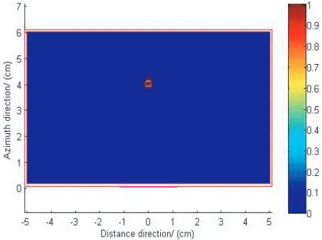
Figure 7. Imaging results by the prediction of the category labels.
of the category labels. The red outline indicates the skin of the human body. Red inner frame express the abdominal wall of human body. The golden box indicates the location of the tumor.
The color block in Figure 7 is the actual location of the tumor target. The actual position and imaging position are relatively consistent. The accurate location of the target is successfully obtained. A virtual shadow exists in the grayscale map of the electric field intensity. The prediction method based on SVM not only eliminates the virtual shadow effectively, but also retains most of the target information. The tumor target information can be predicted when the classification accuracy reaches a certain degree (i.e., the shape of the tumor target has a certain ability to be identified). The classification accuracy of the positive class in this study is 88.674%. The shape and position of the tumor target can be judged properly.
Figure 8. Azimuth direction amplitude distribu-tion.
Figure 9. Distance direction amplitude distribu-tion.
Figure 10. Circular tumor imaging based on BP algorithm.
Figure 11. Square tumor imaging based on BP algorithm.
6.2. Reconstruction of Tumor Models in Different Patients
The stomach presents relatively different shapes, sizes, locations, and quantities of tumors. In this section, simulation experiments and analyses are conducted for these different situations. Only the following changes are made based on the model shown in Figure 1: (1) circular shape of tumor, with the center coordinates of (3.5 cm, 3.2 cm) and diameter of 0.8 cm; (2) square shape of tumor, with center coordinates of (−1.2 cm, 2.8 cm) and length of 0.5 cm; (3) rectangular shape of tumor with center coordinates of (−3.2 cm, 4.4 cm), length of 1 cm, width of 0.3 cm, and tumor located in lateral wall of stomach; (4) three tumors are detected in stomach, with same locations, sizes, and shapes as those of (1), (2), and (3). Figures 5 to 8 show simulation results obtained by BP algorithm.
Figure 12. Rectangular tumor imaging based on BP algorithm.
Figure 13. Multiple tumor imaging based on BP algorithm.
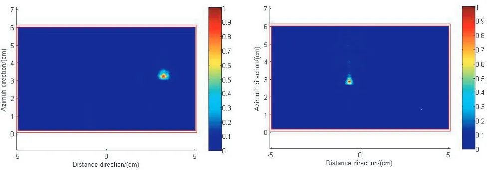
Figure 14. Circular tumor target recognition imaging by SVM based on BP algorithm.
Figure 15. Square tumor target recognition imaging by SVM based on BP algorithm.
caused by mutual interference among tumor targets. Scattering intensity is large when rectangular target tumor size is large but is small when circular and square tumors are smaller. Therefore, imaging of rectangular target is relatively good, but width of distance is smaller than the actual model. Imaging of circular and square targets is slightly poorer. Circular and square targets not only are clear during shape recognition but also manifest a certain offset in the central position.
The model is then predicted by the model BP obtained in a previous section, and results are shown in Figures 14 to 17.
Figures 14 to 17 show that the shapes of tumor targets are predicted more clearly by the model BP. Whether tumor shape is a square, rectangular, or circular, the basic outline remains visible. Mutual interference among tumors decreases in the case of multiple targets, and area of virtual scene decreases. However, electric field intensity of tumor signal and the virtual scene signal present a slight difference. Thus, SVM can detect false virtual scene signals as tumor signals and cannot completely eliminate virtual scenes. Scattering intensity is also large because of the large size of rectangular and circular tumors. Scattering intensity of square tumors is small. Thus, SVM misses square targets.
Figures 13 to 16 show simulation results obtained by F-K algorithm.
Figure 16. Rectangular tumor target recognition imaging by SVM based on BP algorithm.
Figure 17. Multiple tumor imaging by SVM based on BP algorithm.
Figure 18. Circular tumor imaging based on F-K algorithm.
Figure 19. Square tumor imaging based on F-K algorithm.
tumors, but a virtual scene can still be observed. As shown by comparison of Figures 19 and 11, F-K algorithm presents higher resolution in distance direction than BP algorithm, and imaging shows a clear square shape. Figure 20 shows the clear outline of rectangular tumor target, but virtual scenes are also observed. Figure 21 shows less mutual interference between each tumor, and virtual scene is less than the results of BP algorithm.
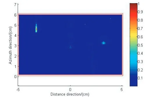
Then, the model is predicted by model F-K obtained in a previous section, and results are shown in Figures 22 to 25.
Figure 20. Rectangular tumor imaging based on F-K algorithm.
Figure 21. Multiple tumor imaging based on F-K algorithm.
Figure 22. Circular tumor target recognition imaging by SVM based on F-K algorithm.
Figure 23. Square tumor target recognition imaging by SVM based on F-K algorithm.
Figure 24. Rectangular tumor target recognition imaging by SVM based on F-K algorithm.
6.3. Signal Polluted by the Noises
The predicted results are based on noise-free conditions. Nevertheless, the data collection process is bound to have noise pollution. Thus, we have to study the signal with the noise.
Table 1. Classification accuracy of the signal after the noise addition.
SNR/dB 5 30 50 No noise
Square
Imaging area 99.937% 99.935% 99.934% 99.937% Negative 99.815% 99.814% 99.812% 99.815% Positive 87.987% 88.323% 88.432% 88.674%
Circular
Imaging area 99.238% 99.237% 99.234% 99.241% Negative 99.801% 99.798% 99.795% 99.804% Positive 46.213% 45.806% 45.684% 46.353%
Rectangle
Imaging area 99.578% 99.572% 99.567% 99.586% Negative 99.476% 99.469% 99.465% 99.489% Positive 88.642% 88.619% 88.573% 88.661%
Two tumors
Imaging area 99.625% 99.618% 99.609% 99.625% Negative 99.574% 99.568% 99.563% 99.575% Positive 89.123% 89.076% 89.055% 89.125%
Table 1 shows the use of the training model to predict the signal of noise pollution. After the addition of different SNR noises, the classification accuracy levels of the positive and negative classes in the imaging area are obtained. The said table shows that the classification accuracy is basically unchanged with the increase in the SNR. This condition shows that the effect of noise pollution on the imaging results is relatively limited. In the imaging region class, the classification accuracy of the negative class is especially high, and the error is 3 bits after the decimal point. This scenario is because the number of negative class samples is much larger than that of the positive class. The classification accuracy of the positive class is slightly lower, especially the circular tumor, which is related to the input data. However, suitable recognition is still obtained.
The relative root mean square error (RMSE) of the abscissa and ordinate of the tumor center is
(a) (b)
defined as follows:
eRMS,x= 1 N N i=1
xiact−xipre lx
2
eRMS,x= 1 N N i=1
yiact−yipre ly
2
(12)
where (xiact, yiact) is the actual location of the tumor target; (xipre, yipre) is the predictive location of the tumor target; lx and ly are the model length and width;N is the number of the test samples.
The proposed method can localize stomach tumors even at low SNR, as shown in Figure 26. As SNR increases, RMSE decreases, and positioning effect improves (i.e., this method is robust).
This section predicts the signal with noise pollution using by the no-noise model. The classification results are basically the same, which shows that the method is robust.
7. CONCLUSION
This study uses FDTD method to simulate gastric tumor model. There will be refraction, reflection and other phenomena when electromagnetic waves travel through the body. A physical propagation model of electromagnetic wave is established to get the correct propagation path of electromagnetic wave. Then, BP and F-K algorithms are used to calculate intensity of each pixel in imaging areas. Intensity of each pixel in imaging area and default category label are marked as input and output of SVM, respectively. SVM model is established after a certain number of tests. Experimental results show that BP and F-K algorithms can locate tumor targets. Imaging featuring the BP algorithm performs poorly because of lack of resolution in distance direction. F-K algorithm presents better effect on shape recognition. However, both methods produce virtual scenes in multitarget imaging because of signal interference. The method based on combination of SVM with BP algorithm can eliminate virtual scenes effectively but may miss targets. The method based on combination of SVM with F-K algorithm can not only eliminate virtual scenes but also accurately locate targets. Based on algorithm efficiency, BP algorithm requires 40 s to 60 s, whereas F-K algorithm takes 1 s. After obtaining characteristic data, prediction of SVM based on the two algorithms lasts for 1 s. Thus, the method based on combination of SVM with F-K algorithm functions better than that based on combination of SVM with BP algorithm and can meet requirements of real-time detection. In the future, the focus of our work is to improve the efficiency of the method and to study the 3D model of the tumor.
ACKNOWLEDGMENT
This work is supported by the National Natural Science Foundation of China 61601245, State Key Laboratory of Millimeter Waves, Southeast University K201724, and China Postdoctoral Science Foundation Funded Project 2016M601693.
REFERENCES
1. Bolomey, J. C., “Recent european developments in active microwave imaging for industrial, scientific, and medical applications,” IEEE T. Microw. Theory, No. 37, 2109–2117, Dec. 1989. 2. National Breast Cancer Coalition (NBCC), URL: http://www.stopbreast- cancer.org, 2014. 3. Yujiri, L., “Passive millimeter wave imaging,” IEEE MTT-S International Microwave symposium,
Vol. 4, 98–101, Jun. 2006.
4. Salmon, N. A., “Polarimetric scene simulation in millimeter-wave radiometric imaging,” Proc. SPIE, 260–269, Feb. 2004.
6. Hu, C., L. Liu, and B. Sun, “Compact representation and panoramic representation for capsule endoscope images,” Int. J. Inf. Acquisit., Vol. 6, 257–268, 2009.
7. Li, B. and M. Q.-H. Meng, “Tumor recognition in wireless capsule endoscopy images using textural features and SVM-based feature selection,” IEEE Trans. on Information Technology in Biomedicine, Vol. 16, No. 3, 323–329, May 2012.
8. Li, B. and M. Q.-H. Meng, “Computer aided detection of bleeding regions in capsule endoscopy images,”IEEE Trans. Biomed. Eng., Vol. 56, No. 4, 1032–1039, Apr. 2009.
9. Li, B. and M. Q.-H. Meng, “Texture analysis for ulcer detection in capsule endoscopy images,”
Image Vis. Comput., Vol. 27, No. 9, 1336–1342, Aug. 2009.
10. Li, B. and M. Q.-H. Meng, “Computer-based detection of bleeding and ulcer in wireless capsule endoscopy images by chromaticity moments,” Comput. Bilo. Med., Vol. 39, No. 2, 141–147, Feb. 2009.
11. Hwang, S. and M. Emre Celebi, “Polyp detection in wireless capsule endoscopy videos based on image segmentation and geometric feature,” Proc. 2010 IEEE Int. Conf. Acoust. Speech Signal Process., 678–681, Mar. 2010.
12. Wang, F. F. and Y. R. Zhang, “Through-wall imaging ultra-wideband radar: Numerical simulation,”Chinese Journal of Radio Science, Vol. 25, No. 3, 569–573, Jun. 2010.
13. Fetterman, M. R., J. Dougherty, and W. L. Kiser, Jr., “Scene simulation of mm-wave images,”
IEEE 2007 AP-S Int. Symposium, 1493–1496, Dec. 2007.
14. Liu, G. D. and Y. R. Zhang, “Three-dimensional microwave-induced thermo-acoustic imaging for breast cancer detection,” Acta Phys. Sin., Vol. 60, No. 074303, 1–7, Sep. 2010.
15. Zhang, H. M., Y. R. Zhang, and F. F. Wang, “Target shape reconstruction method for the through-wall radar based on SVM,”Chin. J. Radio, Vol. 30, 153–159, Feb. 2015.
16. Wang, F. F. and Y. R. Zhang, “An electromagnetic inverse scattering approach based on support vector machine,” Acta Phys. Sin., Vol. 61, No. 084101, 1–8, Jul. 2012.
17. Skjelvareid, M. H., T. Y. Birkelund, and Y. Larsen, “synthetic aperture focusing of ultrasonic data from multilayered media using an omega-K algorithm,” IEEE Transactions on Ultrasonics, Ferroelectrics, and Frequency Control, Vol. 58, No. 5, 1037–1048, May 2011.
18. Vapnik, V.,The Nature of Statistical Learning Theory, Springer-Verlag, New York, 1995.
19. Miteran, J., S. Bouillant, and E. Bourennane, “SVM approximation for real-time image segmentation by using an improved hyperrectangles-based method,” Real-Time Imaging, Vol. 9, 179–188, 2003.
20. Vapnik, V.,Statistical Learning Theory, J. Wiley, New York, 1998.
21. Steinwart, I., “On the optimal parameter choice for v-support vector machines,” IEEE Trans. on Pattern Analysis and Machine Intelligence, Vol. 25, No. 10, 1274–1284, 2003.
22. Mangasarian, O. and D. Musicant, “Lagrangian support vector machines,” Journal of Machine Learning Research, Vol. 1, 161–177, 2001.
23. Wang, L.,Support Vector Machines: Theory and Applications, Springer-Verlag, New York, 2005. 24. Jain, A. K. and D. Zongker, “Feature selection, evaluation, application, and small sample
performance,”IEEE Trans. PAMI, Vol. 19, No. 2, 153–158, Feb. 1997.
25. Dash, M. and H. Liu, “Feature selection for classification,” Intell. Data Anal., Vol. 1, 131–156, 1997.
26. Guyon, I., J. Westion, S. Barnhill, and V. Vapnik, “Gene selection for cancer classification using support vector machines,” Mach. Learn., Vol. 46, 389–422, 2002.
27. Zhang, H. M., Y. R. Zhang, and F. F. Wang, “Target-recognition method for support vector machine on near-field radar imaging,” Journal of Nanjing University of Posts and Telecommunications (Natural Science), Vol. 34, No. 5, 41–46, Oct. 2014.
28. Gurel, L. and U. Oguz, “Three-dimensional FDTD modeling of a ground-penetrating radar,”IEEE Trans. Geosci. Remote Sens., Vol. 38, 1513–1520, Apr. 2008.
29. Wu, S. Y., Y. Y. Xu, and J. Chen, “Through-wall shape estimation based on UWB-SP radar,”
30. Dehmollaian, M., “Through-wall shape reconstruction and wall parameters estimation using differential evolution,”IEEE Geosci. Remote Sens. Letters, Vol. 8, 201–205, Feb. 2011.
31. Chapelle, O., P. Haffner, and V. N. Vapnik, “Support vector machines for histogram-based image classification,”IEEE Transactions on Neural Networks, Vol. 10, No. 5, 1055–1064, May 1999. 32. Cheng, Z., W. Ji, and L. Hao, “Imaging algorithm for synthetic aperture interferometric radiometer
in near field,” Science China Technological Sciences, Vol. 54, 2224–2231, Aug. 2011.
33. Sun, J. G., “F-K demigration in media with constant velocity: Basic concepts, formulas, and applications in inhomogeneous media,”Journal of Jilin University (Earth Science Edition), Vol. 38, No. 1, 135–143, Jan. 2008.
34. Xiu, Z. J., J. Chen, G. Y. Fang, and F. Li, “Ground penetrating radar imaging based on F-K migration and minimum entropy method,” Journal of Electronics and Information Technology, Vol. 29, No. 4, 827–830, Apr. 2007.