AUTOFOCUS ALGORITHMS PERFORMANCE EVALUATIONS USING AN INTEGRATED SAR PRODUCT SIMULATOR AND PROCESSOR
T. S. Lim, C. S. Lim, V. C. Koo, H. T. Ewe, and H. T. Chuah
Faculty of Engineering & Technology Multimedia University
Jalan Ayer Keroh Lama, Bukit Beruang, 75450 Melaka, Malaysia
Abstract—The design and development of synthetic aperture radar (SAR) system for a particular application often requires redesign of software and hardware to optimize the system performance. In addition, evaluations of the performance of existing autofocus and image formation algorithms are required for the SAR system designers to select a most suitable algorithm for a given image quality requirements. This is a time-consuming taskwithout a reconfigurable and comprehensive software package. Thus, a comprehensive SAR integrated simulator and processor software is needed to aid the system designers in optimizing all the system parameters and performance. This paper presents an integrated SAR simulator and processor (iSARSIMP) software package and the performance of three selected SAR autofocus algorithms has been evaluated as examples to demonstrate the usefulness of the iSARSIMP for SAR system designers. In the performance evaluation, simulated and actual SAR raw data were used for further analysis and comparison of the three selected autofocus algorithms.
1. INTRODUCTION
required for the SAR system designer for a selection of a most suitable autofocus algorithm for a given image quality requirements. In addition, the design and development of a typical SAR system often requires redesign of software and hardware to optimize the system performance. Thus, a complete SAR integrated simulator and processor software is needed to aid the system designers in optimizing all the system parameters and performance.
This paper introduces an integrated SAR simulator and processor (iSARSIMP) software package, where it is applied to analyze the performance of three selected autofocus algorithms. The iSARSIMP software is implemented by using Matlabr
application software. A complete simulator would model end-to-end SAR process, including the sensor-target geometry, the antenna and receiver systems, the operation of a signal processor, and the production of a radar image [1, 2]. The developed iSARSIMP is capable to perform mission planning, terrain modelling, autofocus and image processing algorithms evaluations as well as for understanding SAR processes. The iSARSIMP actually is an extension workof earlier developed iSIM simulator package [1]. However, various major enhancements can be found in the iSARSIMP as compared to iSIM. The iSARSIMP is a complete SAR simulator and processor enhanced with three image processing algorithms and various autofocus algorithms. In addition, one-dimensional (1D) and 3-dimensional (3D) SAR images plots also available for image quality analysis. The design of iSARSIMP is based on modular simulation and processing platform, which consists of various independent modules that share a pool of data files. Each module may be developed and executed separately, depending on individual applications.
The data format of iSARSIMP is a simplified version of the CEOS (Committee of Earth Observations Satellites) standard on SAR data set [1, 3]. The SAR data records will use the same data format for all SAR product types [1] in iSARSIMP. By having common formats, users from various working groups would be able to analyze and merge data from multiple resources.
simulated complex data and actual SAR raw data from RADARSAT-1.
2. THE ISARSIMP TOOL
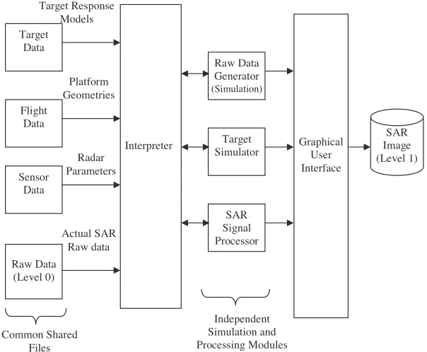
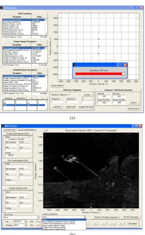
The structure of iSARSIMP is a modular-based SAR simulation and processing platform as shown in Figure 1. It consists of various independent modules that share a pool of data files. Each module may be developed and executed separately, depending on individual applications. In order to exchange data resources, the iSARSIMP requires an interpreter to convert their task-specific results to a common format. Figure 2 shows the main interface of the iSARSIMP. Basically it is consists of two main modules: (a) SAR Simulator module and (b) SAR Processor module.
Independent Simulation and Processing Modules Common Shared Files Radar Parameters Target Response Models Platform Geometries SAR Image (Level 1) Sensor Data Flight Data Target Data Raw Data (Level 0)
Interpreter Graphical User Interface Raw Data Generator (Simulation) Target Simulator SAR Signal Processor Actual SAR Raw data
Figure 1. Structure of modular-based iSARSIMP.
2.1. SAR Simulator Module
(a)
(b)
parameters, (ii) Range domain parameters, (iii) Azimuth domain parameters, (iv) SAR data simulation and (v) Radarsat-1 SAR data extraction. The main function of this module is to assist system designers in designing a SAR system. The design parameters in each sub-module can be modified and saved for a new SAR system design. All the other related parameters in sub-modules will be automatically updated when a particular parameter is modified or changed. The SAR data simulation module is able to generate simulated Level-0 raw SAR data, which is saved in the modified CEOS format [1]. Besides, the Radarsat-1 SAR data extraction module function is to extract a particular area of data from Radarsat-1 raw data [4], which can be saved in Matlabr
mat file format.
2.2. SAR Processor Module
A snapshot of the SAR Processor Module of iSARSIMP software is shown in Figure 2(b). There are three common SAR processing algorithms implemented in this module to process the raw data (level 0) to be SAR image (level 1). The implemented SAR processing algorithms are Range Doppler algorithm (RDA), Chirp Scaling algorithm (CSA) and Omega-K algorithm (ωKA) [4]. In addition, the processed SAR image (level 1) will be displayed on the SAR processor module and can be exported to standard image format such as JPEG. For SAR image quality evaluation and analysis, three focal quality indicators namely (i) 3 dB resolution (3 dBR), (ii) peak sidelobe ratio (PSLR), (iii) signal-to-noise ratio (SNR), (iv) integrated sidelobe ratio (ISLR) and (v) image entropy (IE) of a processed SAR image are provided in this module. Moreover, the inclusion of one-dimensional in range and azimuth domain plots, two-one-dimensional SAR images as well as three-dimensional SAR images plots provide a useful tool for the performance comparison and analysis of various SAR autofocus and image formation algorithms.
3. AUTOFOCUS ALGORITHMS PERFORMANCE EVALUATION USING ISARSIMP
The distance between radar platform and the center of scene being imaged must be known accurately for demodulation of radar returns in a SAR imaging process. When this distance is not measured or known accurately, the SAR data will be corrupted by phase error. The phase error function, θe(y) that varies with each received echo (in azimuth
Fourier transform,Se(X, Y) is given as:
Se(X, Y) =S(X, Y)ejθe(y) (1)
whereXandY are the range and azimuth spatial frequency variables. The SAR autofocus algorithm is to estimate the phase error,θe(y) and
subsequently removes the phase error.
The three selected autofocus algorithms in this performance evaluation using iSARSIMP are phase gradient algorithm (PGA), non-overlapping sub-aperture autofocus (NSA) algorithm and Particle Swarm optimization (PSO) based autofocus [5, 6] algorithm. Various autofocus algorithms have been proposed in the literature over the past 20 years. The most popular and widely utilized is PGA algorithm, which is presented by Eichel et al. in 1989 [7, 8]. PGA determines the phase error by estimates the phase differences between range-compressed SAR data, and subsequently integrates it. It has been shown that a linear unbiased minimum variance (LUMV) estimate of the gradient of the phase error is given by [7]:
ˆ˙
θlumv(y) = N
n=1
Im [ ˙se(y)s∗e(y)]
N
n=1
|se(y)|2
= ˙θe(y) + N
n=1
|se(y)|2θ˙n(y)
N
n=1
|se(y)|2
(2)
where ˙θeand ˙senare, respectively, the first derivative ofθeandse; and
these is shifted and windowed SAR image data.
A more recent algorithm is non-overlapping sub-aperture autofocus (NSA), proposed by [9]. In the basic NSA, the azimuth length is divided into Ka smaller sub-apertures. The unwrapped
phase gradient of each sub-aperture is independently estimated using a conventional optimization approach. Further, the second derivative of the phase is computed to remove the phase-slope discontinuities at the borders of sub-apertures. The algorithm is innovative because it uses a search technique that does not require the computation of a gradient [9]. However, the authors of the algorithm have made no comparison with other autofocus algorithms in for 2D simulated and real SAR data.
Figure 3. Ideal 2D and 1D SAR images plots of the 3 simulated point targets.
Figure 4. Ideal 3D plot of SAR images of the 3 simulated point targets.
3.1. Example 1: Simulated Data
500 m in range domain) SAR image need to be generated using SAR Simulator Module. The reflectivity of the 3 simulated point targets is set at 1.0 (max), 0.8 and 0.6 respectively. All others simulation parameters can be found from Figure 2(a). Figure 3 shows the ideal 2D and 1D SAR images plots of the 3 simulated point targets using Range Doppler Algorithm (RDA) from SAR Processor Module. For better visualization, two 3D plots of SAR images of the 3 simulated point targets are shown in Figure 4. In order to evaluate the performance of the selected autofocus algorithms, a most common phase error, namely low-frequency high-order polynomial phase errors (LF-HPE) is introduced in the simulated SAR image.
(a) (b)
(c) (d)
Figure 5. (a) Simulated SAR image corrupted seventh-order polynomial phase error, (b) Compensated by PGA algorithm, (c) Seventh-order polynomial phase error function (actual phase error), (d) Actual and estimated phase error functions by PGA.
(a) (b)
(c) (d)
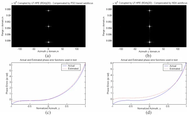
Figure 6. (a) Simulated SAR image compensated by PSO based algorithm, (b) Compensated by NSA algorithm, (c) Actual and estimated phase error functions by PSO, (d) Actual and estimated phase error functions by NSA.
inspection of Figure 5(b) as compared to Figure 5(a) shows significant improvement in the image quality. It can be observed from Figure 5(d) that the phase errors (LF-HPE) in the image have been successfully estimated and subsequently being minimized after compensated by PGA algorithm.
In addition, Figure 6(a) and Figure 6(b) show the compensated 2D SAR image by using PSO based and NSA autofocus algorithms respectively. When comparing Figure 6(a) and (b) with Figure 5(a) by visual inspection, significant image quality improvement can be observed where phase errors almost totally eliminated. From Figures 6(c) and (d), it can be noticed that phase error estimated by PSO based autofocus algorithm is closer to actual phase error as compared to NSA autofocus algorithm.
(a) (b)
(c) (d)
Figure 7. (a) Corrupted simulated SAR image (3D), (b) Compensated by PGA (3D), (c) Compensated by PSO (3D), (d) Compensated by NSA (3D).
In order to evaluate the quality of two-dimensional SAR image, signal-to-noise ratio (SNR), 3 dB resolution (3dBR), peaksidelobe ratio (PSLR) and image entropy (IE) are used as focal quality metrics. The 3 dBR is defined as −3 dB mainlobe of a point target response in the azimuth direction. This is the main performance criterion since the minimum space separation of two points that can be distinguished will determine how well the final image is focused. The PSLR is the ratio between the height of the largest sidelobe and the height of the mainlobe [4]. The PSLR should be kept small to avoid small targets masked by adjacent strong targets. The PLSR is analyzed in one dimension (in azimuth domain) after range and azimuth compression. On the other hand, image entropy is a conventional focal quality indicator used to measure how well an image is focused. As an image becomes blurred or corrupted by phase errors, the IE of the image will increase. Thus, an image is best focused when the value of IE of the image is minimum. An approximation of the IE is given in [5, 11], for SAR data in discrete form as:
IE=−
M−1
m=0
N−1
n=0
sm,nlnsm,n (3)
Table 1 shows the results of the SNR, 3 dBR, PSLR (1D azimuth domain) and IE of the simulated SAR image for the ideal, corrupted by LF-HPE and post-compensation by the selected autofocus algorithms. From Table 1, it is found that PGA algorithm recorded the highest SNR, lowest PSLR and IE value follows by PSO and NSA algorithms. It should be noted that the smaller value of IE indicates better focus of the image. All the selected autofocus algorithms manage to improve the 3 dBR from 4 m (corrupted) to 1 m. The results in Table 1 indicate that PGA recorded the best performance among the three algorithms, follows by PSO and NSA. However, the differences in performance among the three algorithms are rather small. In term of the computational time, NSA is the fastest algorithm while PSO based algorithm recorded the longest time.
Table 1. SNR, 3 dBR and IE of the simulated 2D SAR image.
SNR (dB) 3 dBR(m) PSLR (dB) IE
Ideal SAR Image 6.7383 1 −21.9957 0.154105
Corrupted by LF-HPE
(7-order polynomial) 6.5258 4 −11.2174 0.261200
PGA compensation 6.7965 1 −22.0156 0.154704
PSO based autofocus
compensation 6.7697 1 −20.5156 0.158882
NSA compensation 6.7352 1 −20.1328 0.170616
3.2. Example 2: Actual SAR Data
(a) (b)
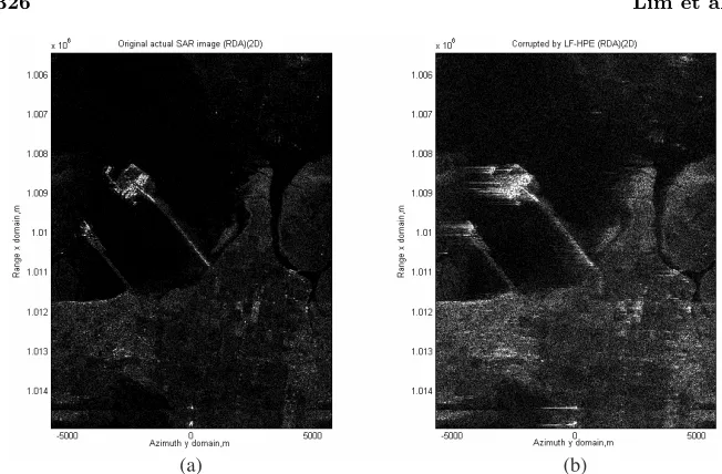
Figure 8. (a) Original actual SAR image from RADARSAT-1 data, (b) Corrupted image.
(a) (b)
Figure 9. (a) Compensated by PGA, (b) Compensated by PSO.
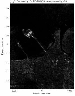
in Figure 8(b). As illustrated in Figure 8(b), the LF-HPE blurs the image and consequently degrades the resolution of the image. The degree of distortion depends on the number of order and value of the coefficients of the polynomial phase error. In addition, Figures 9(a) and 9(b) show the compensated SAR image which was corrupted by LF-HPE by using PGA and PSO based autofocus algorithms respectively. The visual inspection of Figures 9(a) and 9(b) as compared to Figure 8(b) shows that great improvement in the image focus quality after reconstructions of the PGA and PSO based autofocus algorithms. Lastly, the compensated SAR image by NSA algorithm as depicted in Figure 10 also shows significant improvement in the image focus quality as compared to Figure 8(b). However, from Figures 8–10, it can be observed that PGA and PSO algorithms exhibit higher performance as compared to NSA algorithm in the actual SAR image phase errors elimination.
Figure 10. Compensated by NSA.
Table 2. IE of the actual SAR image.
IE
Ideal SAR Image 5.88104
Corrupted by LF-HPE (7-order polynomial) 6.81286
PGA compensation 5.88676
PSO based autofocus compensation 5.89285
NSA compensation 5.94194
best performance in phase error elimination follows by PSO algorithms. However, the NSA algorithm recorded the shortest computational time in phase error estimation while PSO algorithm requires the longest computational time.
4. CONCLUSION
The performance of the three selected SAR autofocus algorithms have been analyzed and compared using an integrated SAR simulator and processor (iSARSIMP) software package. Other than autofocus algorithms performance analysis, the iSARSIMP is also integrated with three popular SAR image formation algorithms (RDA, CSA and ωKA), SAR raw data generator, simulator, output viewer in 1D, 2D and 3D plots options. The developed iSARSIMP is a comprehensive software tool for design, optimize, analyze, simulate and process SAR related product. Thus, it can assist system designers and researchers to evaluate SAR system design, processing techniques, autofocus algorithms and so on for a given SAR system and image quality requirements. The simulated and actual SAR data testing results further validate the potential of NSA and PSO based autofocus algorithms in estimating SAR phase errors with comparable performance with the well-established PGA algorithm.
REFERENCES
1. Koo, V. C., C. S. Lim, and Y. K. Chan, “iSIM — An integrated SAR product simulator for system designers and researchers,” Journal of Electromagnetic Waves and Applications, Vol. 21, No. 3, 313–328, 2007.
“Radar image simulation,”IEEE Trans. Geosci. Remote Sensing, Vol. 16, No. 4, 296–303, 1978.
3. CEOS Working Group on Data, “Synthetic aperture radar data product format standards,” CEOS-SAR-CCT, Issue/Rev: 2/0, 1989.
4. Cumming, I. G. and F. H. Wong, Digital Processing of Synthetic Aperture Radar Data, Artech House Inc., 2005.
5. Lim, T. S., V. C. Koo, H. T. Ewe, and H. T. Chuah, “A SAR autofocus algorithm based on particle swarm optimization,” Progress In Electromagnetics Research B, Vol. 1, 159–176, 2008. 6. Lim, T. S., V. C. Koo, H. T. Ewe, and H. T. Chuah,
“High-frequency phase error reduction in SAR using particle swarm optimization,” Journal of Electromagnetic Waves and Applications, Vol. 21, No. 6, 795–810, 2007.
7. Eichel, P. H. and C. V. Jakowatz, “Phase gradient algorithm as an optimal estimator of the phase derivative,”Optics Letters, Vol. 14, No. 20, 1101–1103, 1989.
8. Eichel, P. H., D. C. Ghiglia, and C. V. Jakowatz, Jr., “Speckle processing method for synthetic aperture radar phase correction,” Optics Letters, Vol. 14, 1101–1103, 1989.
9. Koo, V. C., Y. K. Chan, and H. T. Chuah, “A new autofocus based on sub-aperture approach,” Journal of Electromagnetic Waves and Applications, Vol. 19, No. 11, 1547–1561, 2005.
10. Kennedy, J. and R. C. Eberhart, “Particle swarm optimization,” Proc. IEEE International Conference on Neural Networks, Vol. 4, 1942–1948, 1995.