Computation of the Fields and Potentials for Particle Tracing under
the Effect of Electromagnetic Forces
Christos Tsironis*
Abstract—In this work we describe a model for the computation of the scalar and vector potentials associated with known electric and magnetic fields, as well as for the inverse problem. The formulation is general, but the applications motivating our study are related to the requirements for advanced modeling of charged particle dynamics in plasma-driven electromagnetic environments. The dependence of the electromagnetic field and its potentials in space and time is assumed to be separable, where the spatial part is connected to established solutions of the static problem, and the temporal part is derived from a phenomenological description based on time-series of measurements. We benchmark our model in the simple problem of a finite current-carrying conductor, for which an analytical solution is feasible, and then present numerical results from simulations of a magnetospheric disturbance in geospace.
1. INTRODUCTION
In problems involving electric and/or magnetic fields, there are basically two options regarding the mathematical modeling of the fields in equations of a physical system. The first option, which is more straightforward, is to use the actual vector fields, i.e., the electric and magnetic field (typically denoted asEandB). The second option is to formulate the problem in terms of the scalar and vector potential of the electromagnetic field (usually denoted as Φ andArespectively). The problem formulations emerging from these two options are different in principle, but not directly independent; they are connected via the (physical and mathematical) relations of the fields with the potentials. In fact, taking into account these (known) relations properly, it is always possible to derive each one of the two formalisms starting from the other one (more details in [1]).
An example of how the different formalisms are connected is seen in the problem of charged particle motion in electromagnetic fields. When the problem is solved within Newtonian mechanics, the emerging Lorentz equation involves the electric and magnetic fields along with the particle momentum. On the other hand, when the motions are calculated using analytical mechanics, the Lagrangian and Hamiltonian functions depend on the electric (scalar) and magnetic (vector) potentials. However, the equations of motions derived within the Lagrangian or Hamiltonian formalism are known to be the same as the ones derived from Newton’s laws, the only differences being in the number and the order of the differential equations [2]. In the course of derivation of the motion equations based on each formalism, this equivalence is always reflected to the known field-potential relations.
Naturally, the choice of specific formalism to apply depends not only on the nature of the problem, but also on the targets of the specific research study. Here we refer mostly to problems connected to charged particle dynamics, which will be the subject area of this paper. For problems where the focus is on producing kinematic data (position, velocity, energy, . . . ), to be used for orbit tracking or for the computation of connected ensemble-averaged physical quantities (e.g., radiation spectrum, diffusion
Received 29 September 2019, Accepted 20 December 2019, Scheduled 5 January 2020
* Corresponding author: Christos Tsironis ([email protected]).
scaling), one usually selects to use the Newtonian formalism due to its immediacy in solving for the motions. In case one needs to get involved in a deeper study of the particle dynamics, the Hamiltonian formalism is preferred due to the insight it provides on the properties of dynamical systems (phase-space structure, invariant quantities etc.) [2].
With respect to the modeling of the forces acting on the particles, the choice of formalism described above (and in the spirit analyzed in the second paragraph of this introduction) generally points to the use of the fields in the case of Newtonian formalism and of the potentials in the case of Hamiltonian formalism. However, depending on the force fields involved, there are cases where it is easier (or even necessary) to calculate the potentials instead of the actual fields, independently of the formalism. One of these cases, which is of special interest for this paper, is the modeling of the electric field component generated due to the dynamic variation of the magnetic field flux. The equation of interest here stems from Faraday’s law (i.e., the third Maxwell’s equation): the sum of the electric field’s curl and the magnetic field’s variation rate is equal to zero. However, a more straightforward equation for the electric field may be derived in terms of the potentials, according to which the sum of the electric field, the divergence of the scalar potential, and the variation rate of the vector potential is zero [3].
The straightforward computation of the scalar and vector potentials involves the solution of Poisson differential equations and the calculation of volume integrals with possible singularities (see examples in [1, 3]). The emerging analytical and numerical difficulties can be overcome in cases where the electric current sources of the problem are far from the regions where the fields and/or potentials should be calculated, e.g., in the problem of computing the vector potential around a current conductor. However, in cases where the distribution of the current sources is dense inside the computational space, e.g., in the problem of charged particle motions in magnetospheric plasmas [4], the numerical computations involved are problematic and alternative solution methods should be looked for.
In this work, we construct a model for calculating the electric and magnetic field when the scalar and vector potentials are known from theory or observations, and vice versa. The formulation is not restricted to specific problems, but the proposed applications are relevant to charged particle motions under the effect of electromagnetic forces coming from dynamic plasmas. In our model, the dependence of the electric and the magnetic field in space and time is thought of as separable: the spatial part is modeled using known solutions of static electric/magnetic problems, whereas the temporal part comes from a phenomenological approach using time-series of electromagnetic measurements. Our model is benchmarked against a simple problem with analytical solution, and then numerical results of particle orbits during a magnetospheric disturbance in geospace are shown, with the orbits computed and compared for different scenarios regarding the actual forces affecting the particle dynamics.
The structure of this paper is as follows. In Section 2, a short synopsis of the classical theory for the electromagnetic fields and potentials (including gauge functions and transformations) is presented, and in Section 3, the model for the description of the dynamic electromagnetic fields and potentials is analyzed. In Section 4, the known methods for the computation of the potentials from the fields and vice versa (including our proposed method) are presented and benchmarked, and in Section 5 the application to a space plasma physics problem takes place. Finally, in Section 6, the conclusions of this study are discussed and the steps for future work are mentioned.
2. ELECTROMAGNETIC FIELDS, POTENTIALS AND GAUGES
The classical theory of electromagnetic fields is reflected in Maxwell’s equations [1, 3]
∇ ·E(r, t) = (r, t)
ε0
(1)
∇ ·B(r, t) = 0 (2)
∇ ×E(r, t) = −∂B(r, t)
∂t (3)
∇ ×B(r, t) = μ0J(r, t) +μ0ε0
∂E(r, t)
∂t (4)
EandB may be expressed in terms of a scalar (also called electric) potential Φ and a vector (also called magnetic) potentialA as follows [1, 3]
E(r, t) = −∇Φ(r, t)−∂A(r, t)
∂t (5)
B(r, t) = ∇ ×A(r, t) (6)
GivenE andB, Equations (5) and (6) do not have a unique solution for Φ andA, but there is a degree of arbitrariness in determining the potentials. This is established by a gauge functionλ, and it can be easily proved that the fields are invariant under the following gauge transformation [1, 5]
Φ(r, t) = Φ(r, t)−∂λ(r, t)
∂t (7)
A(r, t) = A(r, t) +∇λ(r, t) (8)
i.e., that applying the above transformation yieldsE =E and B=B.
A characteristic example of the usefulness of the gauge transformations is the simplification of the Laplace equation for the vector potential in magnetostatics. The derivation of the Laplace equations starts by substituting Eqs. (5) and (6) to Eqs. (1) and (4), assuming also that all temporal derivatives are zero. The initial result has the following form [3]
∇2Φ(r) = −(r)
ε0
(9)
∇2A(r) = −μ
0J(r) +∇
∇ ·A(r) (10)
Equation (10) would be simplified if the second term on the right-hand side, which includes a complicated derivative of the unknown potential, was dropped. This may be achieved by choosing a specific gauge level forA, which is known as the Coulomb gauge and is based on the relation ∇ ·A= 0 [5].
For some problems, there are important advantages in using an electromagnetic model in which the properties customarily associated with the fields, like, e.g., the stored energy and the energy flow, are assigned instead to the potentials. For example, the reformulation of Poynting’s theorem on the basis of the potentials provides an energy flow vector which simplifies the quantitative description of electromagnetic power transfer, because it is closely related to the circuital concept and, unlike the Poynting vector, demonstrates also the fundamental importance of electromagnetic forces [6]. This may be equally applied to problems that include charged particle dynamics, where a deeper study of the associated dynamical system (i.e., beyond a simple kinematic tracking of particle orbits, like, e.g., in [7]) is required. In such studies, the Hamiltonian formalism is preferred because it provides an insight of the phase-space structure and the system invariants (as demonstrated, e.g., in [7, 8]). Within this formalism, however, it is more convenient to use the potentials instead of the fields, since these enter directly in the Hamiltonian function as scalar variables [2].
3. DESCRIPTION OF THE ELECTROMAGNETIC FIELD
We present in this section a useful model for space and time-dependent electric and magnetic fields and their potentials, which we will use throughout this paper. This model has a practical simplification, which however is suitable for describing accurately many categories of natural and technical systems: the functional dependencies of the fields and their potentials over space and time are considered to be separable. This assumption opens the way for an easier modeling of the electromagnetic field, since the spatial part may be modeled using the solution of the corresponding electro/magneto-static problem (either known, or anyway obtained with less effort than the one needed for solving the full electrodynamic problem), whereas the temporal part may be obtained in terms of phenomenological approaches involving time-series coming from the electric and magnetic data.
solving Eq. (5) with known E and A, in (ii) B is found from Eq. (6) with known A, and Φ by solving Eq. (5) with knownE andA, in (iii)Ais computed by solving Eq. (6) with knownB, and thenE from Eq. (5) with known Φ andA, and in (iv)Bis found from Eq. (6) with knownA, andEfrom Eq. (5) with known Φ and A. In problems related to the computation of charged particle motions in the presence of electromagnetic forces, which are under focus in our paper, the most frequent scenario occurring is (iii). This is mainly because the magnetic field and the electric potential are, in principle, easier to measure, but also because, in many cases of interest, there are a lot of theoretical models available for these two quantities as compared toE and A(details, e.g., in [9]). Hence, in the following, and without loss of generality (the formalism for the other cases may be derived likewise), we will present our model formulation on the basis of that specific case.
In the context introduced above, the time-dependence of the fields and potentials is described in a logic similar to that of an “event”, i.e., a well-defined set of simultaneous physics processes which are localized in time, starting and ending at specific timestampst1 and t2 respectively. According to this,
we have the following expressions for the magnetic field and the scalar potential [10]
B(r, t) = B(r, t1) +
B(r, t2)−B(r, t1)
b12(t) (11)
Φ(r, t) = Φ(r, t1) + [Φ(r, t2)−Φ(r, t1)]f12(t) (12)
where b12 and f12 are normalized profile functions characterizing the variations of B and Φ, with
b12(t1) =f12(t1) = 0 andb12(t2) =f12(t2) = 1. Equations (11), (12) imply that (i) the values ofB, Φ at
the start and end time of the event may be computed by given models for the physics process, e.g., from solutions to a static problem with input parameters relevant to the dynamical system at the specific timestamps, and (ii) the physics behind the evolution ofB and Φ during the event should be included in the profile functions, which may be computed by fitting against measurements of relevant processes. In case the system dynamics composes of fragments that obey different physics, the ansatz may be generalized to a sum of components described by different profile functions that refer to consecutive events (we analyze this option in the end of this section).
Owing to the separability of the space and time dependencies in Equation (11), the application of Equation (6) for determiningA yields a relation of the following form
A(r, t) =A(r, t1) +
A(r, t2)−A(r, t1)
b12(t) +cA(t) (13)
where ∇ ×A(r, ti) = B(r, ti) (i= 1,2), and cA is an arbitrary function which depends only on time,
yielded from the partial integration of Eq. (6) over space. Without any loss of generality, we can set
cA(t) = 0 in order to simplify our model equations. This option is justified since cA is related to the
choice of gauge level where the vector potential is measured and, in this sense, could be placed out of Eq. (13) in terms of a proper transform [5]. Then, by comparing Eqs. (11) and (13), it is seen that A
is described by a similar type of equation as the one for B. This comes essentially as a result of the fact that the profile functions do not have a spatial dependence (a choice aiming to the separability of the independent variables); so, in case one applies a gauge transform, and since the magnetic fields pre and post-transform are equal, they should also be described by the same profile function (i.e.,
B =B ⇔b =b).
Inserting Equations (12) and (13) into Equation (5), as described after the beginning of this section, gives a first version of the model equation for the electric field
E(r, t) =−∇Φ(r, t1)−[∇Φ(r, t2)− ∇Φ(r, t1)]f12(t)−
A(r, t2)−A(r, t1)
db12(t)
dt (14)
This relation provides a direct approach for the computation ofE with respect to the known quantities Φ andA(as computed using the known values ofB). For the sake of conceptual understanding, it may be written in a similar form to the ones forB, Φ, andA, in Eqs. (11), (12), and (13), respectively. In this direction, first we calculate the electric field values at the timestamps ti (i = 1,2) signifying the
Then, after some algebraic manipulations, Equation (14) becomes
E(r, t) = E(r, t1) +
A(r, t2)−A(r, t1)
db12(t)
dt −
db12(t1)
dt
+
E(r, t2)−E(r, t1)−
A(r, t2)−A(r, t1)
db12(t2)
dt −
db12(t1)
dt
f12(t) (15)
In what has been presented up to now, we have assumed that the system dynamics is dominated by a single event. In cases where a number of electromagnetic processes with different physics are present, the model formulas in Equations (11) and (12), and, consequently, in Eqs. (13), (14), and (15), can be generalized as sums of consecutive events based on different profile functions. As a first step, the fields and the potentials between two timestampsti,ti+1 may be modeled with the following formulas
Bi,i+1(r, t) = B(r, ti) +
B(r, ti+1)−B(r, ti)
bi,i+1(t) (16)
Φi,i+1(r, t) = Φ(r, ti) + [Φ(r, ti+1)−Φ(r, ti)]fi,i+1(t) (17)
Ai,i+1(r, t) = A(r, ti) +
A(r, ti+1)−A(r, ti)
bi,i+1(t) (18)
Ei,i+1(r, t) = E(r, ti) +
A(r, ti+1)−A(r, ti)
dbi,i+1(t)
dt −
dbi,i+1(ti) dt
+
E(r, ti+1)−E(r, ti)−
A(r, ti+1)−A(r, ti)
dbi,i+1(ti+1)
dt −
dbi,i+1(ti) dt
fi,i+1(t) (19)
If one considers a number ofN consecutive events, each one evolving within the timestampsti andti+1
(i = 1,2, . . . , N), the above formulas may be used in conjunction with Heaviside step functions [11] (denoted here withH) for describing the hierarchy of these events in time. Additionally, in cases where it is necessary, lags of pause between the events may be included by setting the corresponding dynamic profile functions equal to zero. Then, assuming the ability to adhere proper definitions for all the profile functions, the fields and potentials of the total process may be expressed in terms of the unified formula
L(r, t) =
N
i=1
H(t−ti)H(ti+1−t)Li,i+1(r, t) (20)
In Eq. (20), L symbolizes each one of the fields and potentials, i.e., it stands for either B, Φ,A orE. It should be clear that if one manages to have available the time-dependent profile functions and the space-dependent boundary values for two out of the four fields and potentials (as analyzed in the second paragraph of this section), then the problem of fully describing the electromagnetic forcing is solved. The boundary functions are actually snapshots of the dynamic quantities and can be calculated as solutions of properly associated electrostatic and/or magnetostatic problems. In this respect, and in order to simplify each problem when necessary, gauge transformations may be used in order to express the quantities of interest more conveniently. On the other hand, the dynamic profile functions may be either prescribed in terms of empirical models or calculated/computed on the basis of time-series data coming from electromagnetic data (measurements, models etc.). In the next section, we present and analyze different techniques for tackling the two aforementioned issues.
4. METHODS FOR CALCULATING THE FIELDS AND POTENTIALS
4.1. Calculation of the Dynamic Profiles
The mathematical functions used for the modeling of the dynamic evolution of the electromagnetic fields and potentials might be determined in two ways: (i) empirical formulas or phenomenological models, and (ii) curve fits of electromagnetic time-series data. In all circumstances, these functions will depend on the temporal evolution of the parameters affecting the specific electromagnetic component (i.e., the dependence of these parameters on time); for example, in space plasma studies, the magnetic field depends on parameters such as the geomagnetic index, the storm-time index and the dynamic solar pressure ([12] and references therein). This aspect should definitely be taken into account, in some way, to the modeling, in order to derive a consistent description of the associated phenomena.
Phenomenological models describe physical processes according to existing empirical knowledge and relations, which are not directly derived from theory (i.e., from first principles) but in a way which is consistent with fundamental theory. In practical applications, such a model for our problem would attempt to define the profiles in terms of smooth (i.e., continuous and differentiable in the variable regions of interest) analytical functions of time, taking into account any restrictions and boundary conditions of the process. As an example, we mention the case where the values of the magnetic field or the scalar potential at two time instants are known; then, one may assume that the evolution of the component in the time lag between these two instants is linear, polynomial, exponential, sinusoidal etc., and define accordingly the profile functions.
In cases where time series of measurements are available, these can be used to produce the necessary profile functions via a fitting procedure (the reader is pointed to [15]). To present the formalism, we assume that the field/potential component L(r, t), with associated profile functions per event li,i+1(t)
(cf. previous section), depends on time only implicitly through theMparametersGj(t) (j = 1,2, . . . , M).
In this frame, the quantity L takes the alternative form L(r, t) = L[r, Gj(t)], and its full derivative over
time may be written as follows [11]
dL(r, t)
dt =
M
j=1
∂L(r, t)
∂Gj ·
dGj(t)
dt (21)
In order to make Equation (21) more suitable for numerical computations, one performs a discretization. Having available data, the established procedure is to define the discretization step Δtaccording to the resolution of the measurements. The discrete formula is the following
L(r, t+ Δt)−L(r, t) =
M
j=1
{L [r, Gj(t+ Δt)]−L [r, Gj(t)]} (22)
and may be seen as a direct consequence of the differentiation chain rule, which says that the total variation is the sum of the variations due to each one of the parameters [11]. By comparing Eqs. (21) and (22), one obtains a realistic estimation of the “global” profile function l(t) for the total simulation interval [t1, t2], as the cumulative result of the dynamics induced from the functions per time lagli,i+1
l(t) =
M
j=1
{L [r, Gj(t)]−L [r, Gj(t1)]}
M
j=1
{L [r, Gj(t2)]−L [r, Gj(t1)]}
(23)
Notice that the profile function, apart from being computed from measured values of L, could also be calculated on the basis of values provided by a theoretical model; for example, in space plasma applications, a Tsyganenko model for the magnetic field could be employed [13].
4.2. Solving the Static Electric and Magnetic Problems
when the fields vary slowly within the time frame of the event, or where the description handles the time dependence separately from the spatial field distribution (see the model presented in the previous section). In such cases, one may use the solutions of the associated static problems for the determination of the spatial part of the fields/potentials; in exact, these are the terms L(r, ti) in Eq. (20) and the
previous four equations. These solutions emerge from the equations of electrostatics/magnetostatics, which, in their turn, stem from Maxwell’s equations after eliminating all time derivatives [1, 3].
The standard theory towards the calculation of the electromagnetic fields and potentials in static problems has been set in the Coulomb gauge (cf. Section 2, and details in [3]). In this gauge, combining Equation (10) with the static version of Eq. (4) and taking into account that ∇ ·A = 0, one gets to ∇2A=−∇ ×B. The solution of the specific partial differential equation forA is written as [1]
A(r) =
VS
∇×B(r)
|r−r| d
3r (24)
whereVS is the volume of the problem space. In the same manner, by combining Equation (9) with the
static version of (1), one may derive the differential equation∇2Φ =−∇ ·E, which, analogously to the previous one forA, has the following solution for Φ [1]
Φ(r) =
VS
∇·E(r)
|r−r| d
3r (25)
Notice that Equations (24) and (25), together with the static versions of Equations (5) and (6), i.e.,
E=−∇Φ andB =∇ ×A, provide solution to all versions of problems mentioned in Section 3.
The technique described above is convenient for many classes of problems relevant to physics and electrical engineering, like, e.g., the determination of the vector potential due to the current flowing in conductors (straight wire, circular loop etc.) around their surrounding space [3]. However, in a variety of physics problems where the charge and/or current sources are scattered inside the volume in which we intend to find the fields/potentials, integrals of the above type are hard to compute due to the poles at the denominatorr−r. Technically, one way to handle the numerical problem atr =r would be to remove the corresponding discontinuity by redefining the integrals as follows
Θα[L(r)] = VS
L(r)
|r−r|2+α2d
3r (26)
In this framework, Equations (24) and (25) may be formulated like A = limα→0Θα(∇ ×B) and
Φ = limα→0Θα(∇ ·E) respectively, and the computation (analytical or numerical) may involve a very
small value ofαset empirically or determined after convergence check. In applications, an investigation whether α can be connected to parameters of the system physics (in plasmas, e.g., Debye screening distance, collision mean free path, thermal Larmor radius etc. [14]) would be of special interest.
More rigorously, the problem may be solved by moving from the Coulomb gauge to another electromagnetic gauge where the computation of the required potentials is more simple. One such option is the Poincare gauge, which is governed by the relation r·A = 0 [5]. In the following, using primes as in Equations (7) and (8), we denote the potentials in the Coulomb gauge (i.e., before the transformation) as unprimed and the ones in the Poincare gauge (i.e., after the transformation) as primed. The relations of the potentials with the fields in the Poincare gauge are [5]
A(r) = −r×
1
0
B(ur)udu (27)
Φ(r) = −r·
1
0
E(ur)udu (28)
which replace Eqs. (24) and (25) respectively in the solution technique described above. Furthermore, based on Equations (7) and (8), the gauge function for the transition between the gauges may be calculated by ∇2λ=∇A, whereas Φ is equal to Φ since λdoes not depend on time.
verification for our method, because there is has an analytic solution for Ain the Coulomb gauge, and consequently B is also known. The corresponding formulas are [1, 3]
Awc(r) = − μ0Iwc
2π ln
ρ2+L2
w+Lw ρ
ˆ
z (29)
Bwc(r) = μ0Iwc
2π Lw
ρ
1
ρ2+L2
w
ˆ
φ (30)
In the above,Iwc is the electric current flowing in the conductor, 2Lw is the length of the wire, and we
use a cylindrical coordinate system (ρ, φ, z). Notice here that, in the limiting case of infinite length for the wire (Lw ρ), one obtains the familiar formulaBwc=μ0Iwc/2πρfor the magnetic field amplitude,
which is actually a consequence from Biot-Savart’s law [3]. In this example, we use the solutions in Eqs. (29) and (30) for proving that the vector potential in the Poincare gauge yields the same magnetic field with the vector potential in the Coulomb gauge, as given in Equation (30).
The first step is to insert Equation (30) into Equation (27), in order to calculate the vector potential in the Poincare gauge. After some preliminary algebra, we obtain the intermediate result
Awc(r) =−r×φˆ μ0Iwc
2πρ
1
0
u2ρ2 L2
w+u2ρ2+Lw
u2ρ2+L2
w
du (31)
The integral in Eq. (31) is calculated more easily by changing the integration variable to υ = uρ/Lw.
By performing a series of manipulations, taking into account thatr×φˆ=ρzˆ−zρˆ[11] and the integral
(1 +υ2+√1 +υ2)−1υ2dυ = ln(υ+√1 +υ2) [15], one gets to the final result
Awc(r) =− μ0Iwc
2π ln
ρ2+L2
w+ρ Lw
zLw ρ2 ρˆ−
Lw ρ ˆz
(32)
A comparison of Equations (29) and (32) manifests important differences between the expressions of the vector potential in the two gauges. Apart from the different arguments in the logarithmic functions,
A is seen to have also a radial component, in contrast to A which has only an axial component. Nevertheless, by applying the established relation for calculating the magnetic field when the vector potential is known (B = ∇ ×A), one manages to obtain the exact same result as in Equation (30), i.e., B =B. The latter completes our verification sequence.
Within a selected description for the dynamic variation of the fields and potentials (details in the previous subsection), the computation of the vector potential opens the way for the determination of the electric field; this is done using either Equation (15) or (19), depending on the case. For applications (see, e.g., next section), we have developed a simple computer code in Fortran 95 for the numerical computation of the vector potential in the two gauges, given the magnetic field either as an analytic model or as tabulated values. In the Coulomb gauge, the code evaluates Equation (24), using the technique reflected by Equation (26) for a specified value of the small parameterα, whereas in the Poincare gauge the code implements Equation (27). The corresponding integrals are computed using standard numerical integration techniques (e.g., Euler’s method, trapezoidal rule, Gaussian quadratures [16]), for the selection of which the user has an option in the input definition.
As a test for the code, we have computed the magnetic field of the straight-line wire conductor, based on the vector potential both in the Coulomb and in the Poincare gauge, and have compared the results with the analytic formula of Equation (30). Regarding the actual computation ofBwc from Awc
andAwc, we have patched an additional routine to our code that finds the curl components of an input
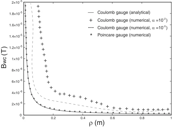
vector, given its values on a discretized grid. In Figure 1 we visualize the results of the computation under the different methods, by plotting the computed magnetic field as a function of the radial distance from the conductor. For the specific computation, the parameters of the wire conductor had values equal to Lw = 5 m andIwc= 1 A, whereas we examined two cases for the parameterα, in which it was equal
0 2×10⁻⁶ 4×10⁻⁶ 6×10⁻⁶ 8×10⁻⁶ 1×10⁻⁵ 1.2×10⁻⁵ 1.4×10⁻⁵ 1.6×10⁻⁵ 1.8×10⁻⁵ 2×10⁻⁵
0 0.2 0.4 0.6 0.8 1
B
wc
(T
)
ρ (m)
Coulomb gauge (analytical)
+ Coulomb gauge (numerical, α =10-2 )
* Poincare gauge (numerical)
* * * * * * * * * * * * * * * * * * * * * * * * * * * * * * * * * * * * * * * * * * * *
--- Coulomb gauge (numerical, α =10-5 ) + + + + + + + + + + + + + + + + + + + + + + + + + + + + + + + + + + + + + +
Figure 1. Comparison of different calculations for the magnetic field of a straight-line conducting wire (Lw = 5 m, Iwc= 1 A) as a function of the radial distance from the wire.
5. APPLICATION TO THE MODELING OF MAGNETOSPHERIC SUBSTORMS
Here we apply the methods already shown to the description of the effects of electromagnetic disturbances to the plasma populations of the Earth’s magnetosphere. We briefly describe an existing particle tracing model for geospace studies and, based on the principles for modeling the dynamic fields (as presented in Section 4), we address the necessary updates in order to include the electric field coming from Faraday induction in the physics description given by sophisticated magnetic field models. Charged particle trajectories during a magnetospheric substorm in geospace are visualized and, for consolidation purposes, compared with orbits computed without the presence of the inductive electric field.
5.1. Overview of the Particle Tracing Model
Whenever the solar wind enters into the Earth’s magnetosphere, space weather effects like geomagnetic storms and magnetospheric substorms are triggered (excellent reviews are [17, 18]). Geomagnetic storms occur when the energy transfer from the Sun to geospace intensifies as a result of magnetic reconnection [17], whereas magnetospheric substorms are connected to the variability in the orientation of the interplanetary magnetic field ([19] and references therein). Both events evolve as energy loading-dissipation cycles, and bring up a configuration change in the magnetosphere by enhancing its current systems [18, 21]. The associated dynamic processes evolve in a variety of timescales, from days for storms to hours, or even minutes, for substorms. In this respect, among the modeling requirements are the consistent description of the electromagnetic fields and the computation of the solar-driven plasma dynamics under these circumstances.
A modeling option is to follow directly the full particle orbits under the electric and magnetic forces during the phases of the event. In such models, the Lorentz equation of motion is solved, either in its full form or reduced in terms of the guiding-center approximation, and the standard physics included is the magnetic field coming from the Earth’s terrestrial magnet plus the fields generated by the magnetospheric currents, and the electric field owed to large-scale plasma convection and corotation with the Earth (e.g., [10, 20]. An important factor, however, is the electric field induced by the time variation of the magnetic field, as it is involved in the strong acceleration of charged particles which is observed during geomagnetic disturbances [19]. In the following, we briefly present the capabilities of the current version of the particle tracing model (for more details the reader is pointed to [10]).
magnet placed at the planet’s center, tilted at an angle θt = 11.5◦ and reversed magnetic poles with
respect to the geographic ones. The formula in Geocentric Solar Magnetospheric coordinates is [10]
Bdip(r) =
BER3E r5
3x(xsinθt+zcosθt)−r2sinθt
ˆ
x
+ [3y(xsinθt+zcosθt)] ˆy+
3z(xsinθt+zcosθt)−r2cosθt
ˆ
z (33)
RE = 6378 km being the Earth radius and BE = 31000 nT the magnetic field strength on the planet’s
surface. In the componentBextgenerated by the electric current systems of the inner magnetosphere, the
most important contributions come from the magnetopause, the magnetotail, the Birkeland regions and the ring current [9]. Our model employs the Tsyganenko routines T89, T96 and TS05, which incorporate physics principles to a data-based description stemming from satellite measurements, and provide the magnetic map of the region under study [13]. In T89, a physics-based description of the magnetospheric currents and the corresponding vector potential was introduced; the T96 model improved T89 in the description of the magnetopause geometry and the equatorial tail physics, whereas TS05 upgraded T96 with the inclusion of storm and substorm dynamics. As far as physics parameters are concerned, what is required at input for T89 is the geomagnetic indexKp, and for T96, TS05 the solar wind pressurePdyn,
the disturbance storm-time index Dst and the components of the interplanetary magnetic field Bimf
transverse to the Sun-Earth direction (the reader is referred to the very good review [13] for details). For the electric field, the sum of the two components is described in terms of a scalar potential Φcc, for the computation of which a variety of physics models has been developed. The most important
are: (i) the Volland-Stern-Maynard-Chen (VSMC) model, based on an empirical dawn-dusk potential distribution withKp-dependence and magnetopause shielding [22], (ii) the Boyle-Reiff-Hairston (BRH) model, which describes the convection field with a polar-cap potential function driven by the solar wind and the interplanetary magnetic field [23], and (iii) the Weimer (WM) model, which is derived from a combination of low-altitude measurements of the convection velocities at high latitude [24]. In our code the VSMC model is employed, because it combines accuracy in the physics description with simplicity in the computer implementation. According to that model, Φcc is approximated as [22]
Φcc(r) =
1
(2Kp2+3Kp+ 1)3
· yr
R2
E
−ωEBER3E
r (34)
with ωE = 2π/24 h−1 the Earth’s rotation frequency and1 = 0.045 kV/m2, 2 = 0.0093, 3 =−0.159
constants that have been fitted over magnetic measurements in the inner tail region. In Equation (34), the first term is the convective potential, in which the fraction involvingKpdetermines the field intensity, and the other term is the potential generating the corotation field.
The magnetic field dynamics is formulated with the scope to describe events with an initial growth period, where the field strength increases to high values, followed by a shorter relaxation phase where the field values return to their quiet-time levels [19]. In this context, Bdip varies slowly in comparison
to the solar activity and its geomagnetic response, so it has been assumed as time-independent. The formulation is along the guidelines of Subsection 4.1: the event sets off at t = ti, grows up to t= tg
and relaxes until its end (t=tf). AsBext depends on the modification of the geomagnetic parameters,
introducing the row matrix G = [Gj] for the input parameters required by each Tsyganenko model
(e.g., [θtKp] for T89), its time derivative is cast in the form of Eq. (21). We remind that the functions Gj(t) may be specified analytically or as tabulated values (i.e., with derivatives computed as finite
differences). In principle, the terms ∂Bext/∂Gj are not available in analytic form, but are obtained
at discrete timestamps by repeated usage of the numerical field model. However, in this fashion, the computing cost increases significantly. In order to simplify the computation, we approximate the dynamic variation ofBextin [ti, tf] in terms of a polynomial-based functionbif (cf. Section 3) [10]
bif(t) =H(t−ti)H(tf −t)
H(tg−t) K
k=1
wk
t−ti tg−ti
k
+H(t−tg) K
k=1
wk
tf −t tf −tg
k
(35)
where wk are a set of K fitting coefficients over ground and satellite data, which for our problem have
For the dynamics of the electric field, we mention first that the slow time-scale of the convection and corotation processes, in comparison to the overall solar-driven plasma dynamics, allows for their consideration as static. As a consequence, and similarly to the Earth’s magnetic field, the scalar potential Φcc has been assumed as time-independent in our model. The time dependence of the electric field
lies in the temporal variation of the external magnetic field, which brings upon an additional electric component as described by Faraday’s induction law. According to Equation (5), this component is given by Eext=−∂Aext/∂t, whereAext is the vector potential forBext. The role of this component in
modeling properly the dynamics of the solar-perturbed geomagnetic plasma is currently established to be important. This is explained via the fact that it has short space/time scales, which is effective in accelerating ions to very high energies, as observed during storms and substorms, whereas the convection process forms a distribution of plasma currents of comparatively low energy (see [19] for details).
The dynamic evolution of the vector potential during the event is described via a relation similar to Eq. (13), where, accordingly, the profile function bif and the values Aext(ti) andAext(tf) enter. In
conjunction with Equation (14), it stems that the dynamic variation of the electric field is quantified in terms of the derivative of the profile function, whereas the required values of the vector potential may be calculated from the solution of the corresponding static problem. Regarding the latter, it is known that an analytic solution for the vector potential, given arbitrary magnetic field, is in most cases not possible. This is the reason why, in the current model, the option of the induced field is available only when the magnetic field model T89 is used, which involves simplifications in the description of the plasma current sources that allow the analytic calculation ofAext[13]. For including the vector potential
calculation in the case of the later models T96 and TS05, which have more complicated formulations (e.g., spherical harmonic expansion, integrals of special functions) with no analytic expression available, we have updated the particle tracing model with the numerical methods presented in Subsection 4.2.
In the framework given above, where (i) the event evolves in phases determined by the values of
G at the timestamps t= ti and t =tf, (ii) the Earth’s dipole magnetic field and the magnetospheric
convection-corotation scalar potential are considered static with respect to the disturbance time scales, (iii) the external magnetic field is described by the normalized profile functionbif, and (iv) the
Faraday-induced electric field is calculated on the basis of the vector potential generating the external magnetic field, the total magnetic and electric fields are finally expressed as
Btot(r, t) = Bdip(r) +Bext
r,G(ti)
+
Bext
r,G(tf)
−Bext
r,G(ti)
bif(t). (36)
Etot(r, t) = −∇Φcc(r)−
Aext
r,G(tf)
−Aext
r,G(ti)
dbif(t)
dt . (37)
These formulas may be easily adapted to codes for the computation of the electromagnetic field in geospace or for other relevant applications, like, e.g., test particle codes and wave dispersion codes.
The particle tracing method performs precise trajectory calculations of near-Earth plasma electrons and ions during the magnetospheric activity growth and relaxation phases. These computations are performed by solving the Lorentz equation of motion, which fully describes the charged particle orbit under the effect of the associated electric and magnetic fields, including also the gravitational force [14]
md
2r
dt2 =q
E(r, t) +dr
dt ×B(r, t)
−mg(r) (38)
In Eq. (38), g(r) = gER2Er/rˆ 2 is the gravitational acceleration (gE = 9.81 m/s2 is its value on Earth’s
surface), andm,q are the particle mass and electric charge. For electrons it isme= 9.31·10−31kg and qe =−1.6·10−19Cb, while for an ion of atomic massAi and ionization rate si it ismi = 1837Aime and qi =si|qe|. The computation is interrupted in case the particle leaves far from the inner magnetosphere,
either by (i) crashing onto Earth (r≤RE), (ii) crossing the magnetopause, or (iii) reaching a tailward
distance further than 70RE. There are different stop codes so that each case is distinguished [10].
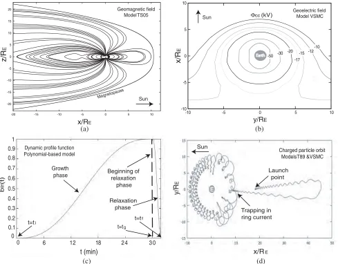
In Figure 2 we provide an overview of results from the particle tracing code, which combines the models presented up so far. In the top-left subfigure, the magnetic field map is displayed using the model TS05 for the external magnetic field, whereas in the top-right subfigure the electric equipotential surfaces are shown using the model VSMC for the convection-corotation field. In the bottom-left subfigure we plot the dynamic profile function bif, and finally, in the bottom-right subfigure, we show an ion orbit
Geomagnetic field Model TS05
-20 -15 -10 -5 0 5 10 15 20
-20 -15 -10 -5 0 5 10
Magnetopau se
Earth
Geoelectric field Model VSMC
x/R
E
y/RE
-10 -5 0 5 10
-10 -5 0 5 10
-50
-10 -20
-17 -15 -12
Φcc (kV)
Sun
-30
Sun
6 12 18 24 3 0
0 1
t (min)
bi
f
(t)
0.9 0.8
0.7
0.6
0.5
0.4
0.3
0.2
0
0.1 t=ti
Growth phase
Relaxation phase Beginning of
relaxation phase
t=tf
t=tg
Sun
x/RE
y/R
E
Dynamic profile function
Polynomial-based model Charged particle orbitModels T89 & VSMC
Earth
E
Trapping in ring current
Launch point
x/RE
z/R
E
(a) (b)
(c) (d)
Figure 2. Overview of results from the particle tracing code for the solar-driven magnetosphere of Earth: (a) magnetic field map of the geospace region, (b) equipotential surfaces of the electric field, (c) dynamic profile function for the magnetic field of the disturbance event, (d) electromagnetic field-driven ion orbit during the disturbance.
5.2. Numerical Results
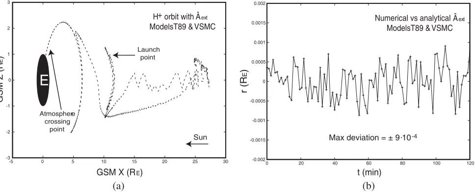
As an example for the problem described in the previous subsection, we present indicative numerical results from charged particle orbits during a substorm in the Earth’s magnetosphere. The main axis of our presentation is along the comparison of trajectories with the same initial conditions and under the same geomagnetic disturbance parameters, as computed both in the presence as well as in the absence of the Faraday induction electric field. Within these results, we first verify the consistency of our computational method by comparing orbits based on the T89 model, with the vector potential calculated using our numerical algorithm vs the corresponding analytical solution (details for the latter may be found in [13]). Then, we visualise examples of orbits computed with the models T96 and TS05, focusing on the differences which are owed solely to the inclusion of the induced electric field model.
For the first part of our simulations, we consider a substorm event that starts atti = 0 with a quiet
magnetosphere, indexed with Kp(ti) = 1, and peaks after tg−ti = 25 min by reaching a disturbed
state with indexKp(tg) = 5. The relaxation phase follows immediately and completes aftertf−tg = 5
min, during which Kp returns to its initial value, i.e., Kp(tf) = Kp(ti). The particle followed is a
-3 -2 -1 0 1 2 3
-5 0 5 10 15 20 25 30
t (min)
r
(R
E
)
GSM X (RE)
GSM Z (R
E
)
E
Sun
H+ orbit with Aext
Models T89 & VSMC
Launch point
Atmosphere crossing
point
-0.002 -0.0015 -0.001 -0.0005 0 0.0005 0.001 0.0015 0.002
0 20 40 60 80 100 120
Numerical vs analytical Models T89 & VSMC
Max deviation = ± 9 10. -4
-A-ext
(a) (b)
Figure 3. Results from particle tracing simulations during a magnetospheric substorm: (a) orbit of an
H+ ion moving from t
0 = 0 untilt1 = 120 min during a disturbance with tg = 25 min, tf = 30 min, as
computed with the T89 model and numerical vector potential, (b) Difference of the orbit radius along the trajectory as computed with the T89 model and numerical vs analytical vector potential.
and then continues moving under the effect of the restored fields until the timestamp t1 = 120 min.
The initial conditions of theH+ ion are the following: (i) radiusr(t0) = 10RE, (ii) magnetic local time ϕ(t0) = 24 h, (iii) latitude θ(t0) = 5◦, (iv) pitch angle ψ(t0) =π/2, (v) kinetic energy Ek(t0) = 1 keV.
In Figure 3 we present results from the test particle simulations, as computed using T89 for the external magnetic field and the numerical model for its vector potential (the latter applied for the determination of the induced electric field). In the subfigure on the left, we show the projection of the ion trajectory on the x-z plane. We notice that the specific particle changes direction after moving tailwards for some time before the event’s peak, then it becomes accelerated and ends up being precipitated in the Earth’s atmosphere over the North Geographic Pole. The computation setup here, apart from an example of the implementation of the numerical model for the vector potential, is also suitable for verification of the model. This is because, as mentioned also above, in the specific case there is an analytic solution available (and included in the T89 output). In this respect, we have computed again the same orbit using the analytical model for Aext and compared with the previously plotted
computation, and in the subfigure on the right we show the difference of the ion radius as a function of time (i.e., along the trajectory). The comparison yields a sufficient accuracy for the numerical method, with the maximum relative deviation of the two results never exceeding 10−3.
The second part of our simulations is focused on the coupling of the induced electric field model to more recent magnetic field models than T89, namely T96 and TS05 in this work. The magnetospheric disturbance considered here is quite similar to the previously studied one, however the choice of physics parameters is now aligned to the Tsyganenko models later than T89. The event sets off at ti = 0,
when the magnetosphere is quiet and described by the parameter valuesPdyn= 1.5 nPa,Dst=−10 nT
and Bimf = 0.2ˆy+ 0.1ˆznT, and grows maximized after tg−ti = 40 min with the physics parameters
reaching their extremum values of Pdyn = 5 nPa, Dst = −90 nT and Bimf = −2ˆy−1.5ˆznT. The
relaxation phase of the event follows immediately and completes after tf −tg = 10 min, during which
all parameters return to their initial values. The particle traced in this case is an oxygen ion, which starts its motion att0=ti, interacts with the disturbed fields untilt=tf and then continues its motion
under the effect of the restored fields untilt1 = 180 min.
In Figure 4 we show the x-z projection of an ion trajectory, which has been computed using the T96 model forBextboth in the presence of the induced electric field (subfigure on the left) as well as in
its absence (subfigure on the right). TheO+ ion has the following initial conditions: (i) r(t0) = 20RE,
GSM X (RE)
GSM Z (R
E
)
Sun
O+ orbit with ext
Models T96 & VSMC
Launch point
10 5 0 5 10 15 20
-10 0 10 20 30 40 50 60 70
Magnetopause crossing
point
E
-10 -5 0 5 10 15 20
-10 0 10 20 30 40 50 60 70
GSM X (RE)
GSM Z (R
E
)
E
Launch point
Sun
O+ orbit without ex t
Models T96 & VSMC
A- A
-(a) (b)
Figure 4. Results from particle tracing simulations during a magnetospheric substorm: (a) trajectory of anO+ion moving fromt0 = 0 untilt1= 180 min, including the disturbance withtg = 40,tf = 50 min,
as computed with the T96 model for the external magnetic field (a) including the induced electric field term and (b) excluding this term.
GSM X (RE)
GSM
Y (R
E
)
Sun
O+ orbit with ext
Models TS05 & VSMC
Launch point
Trapping in ring current
GSM X (RE)
GSM Y
(R
E
)
Launch point
Sun
O+ orbit without ext
Models TS05 & VSMC
-20 -15 -10 -5 0 5 10 15
-15 -10 -5 0 5 10 15 20 25 30
E
-20 -15 -10 -5 0 5 10 15
-15 -10 -5 0 5 10 15 20 25 30
E
A- A
-(a) (b)
Figure 5. Results from particle tracing simulations during a magnetospheric substorm: (a) trajectory of anO+ion moving fromt0 = 0 untilt1= 180 min, including the disturbance withtg = 40,tf = 50 min,
as computed with the TS05 model for the external magnetic field (a) including the induced electric field term and (b) excluding this term.
we notice that the two computations yield a quite different physics picture: whenEextis not taken into
account, the ion is moderately accelerated and remains trapped in the inner magnetosphere, whereas, with the inclusion of Eext in the modeling, the ion is strongly energized and exits the inner geospace
region through the magnetopause. This contradiction in the results illustrates the advantages of our treatment in the spirit of developing more accurate models for relevant processes.
θ(t0) =−10◦, (iv) ψ(t0) =π/2, (v) Ek(t0) = 7 keV. A comparison of the two subfigures yields, also in
this case, a different outcome in the results. First, when the induced electric field is taken into account, the ion is accelerated intensely during the growth phase of the disturbance and finally gets trapped in the ring current plasma population surrounding Earth. In the second case, whereEextis not taken into
account, the ion shows a trend to follow a similar orbit, however its motion is such that it does not incorporate into the ring current until t = t1. The deviation of the results is not as large as the one
of the scenario shown in Figure 4; however, this deviation depends also on the disturbance parameter and the particle initial conditions, including the type of ion (i.e., electric charge and atomic mass), and therefore it could be more intense for another selection of these parameters.
6. CONCLUSIONS
In this paper, we have analysed a bundle of models for the computation of the scalar and vector potentials associated with known electric and magnetic fields, and vice versa. Our work has been motivated by the current requirements for advanced modeling of charged particle dynamics involved in plasma-related electromagnetic environments. Our formulation is, in principle, general, apart from the hypothesis that the space-time dependence of the electromagnetic field and its potentials is separable. This scenario, which is very often met in space plasmas when studying the solar-driven planetary magnetospheres, allows to link the spatial part to known solutions of static problems and the temporal part to phenomenological modeling based on physics data. A numerical implementation of our model, after being benchmarked against the simple problem of a finite current-carrying conductor (i.e., with an analytic solution), was applied to the simulation of typical magnetospheric disturbances in geospace. Apart from a flexible numerical method for the computation of the scalar and vector potentials in problems where the corresponding solutions in the Coulomb gauge are inconvenient, the present work may serve as an option for the modeling of the Faraday induction electric field in problems where it is required. As future work, we intend to use our model, in conjunction with sophisticated models of the planetary magnetospheres, for the improvement of the accuracy in the modeling of electromagnetic disturbances and the assessment of the associated effects.
REFERENCES
1. Jackson, J. D., Classical Electrodynamics, 3rd edition, Wiley, New York, 1999. 2. Goldstein, H., Classical Mechanics, 2nd edition, Addison-Wesley, Boston, 1980.
3. Griffiths, D. J., Introduction in Electrodynamics, 4th edition, Addison-Wesley, Boston, 2012. 4. Parks, G. K.,Physics of Space Plasmas: An Introduction, Addison-Wesley, New York, 1991. 5. Jackson, J. D., “From Lorenz to Coulomb and other explicit gauge transformations,”Am. J. Phys.,
Vol. 70, 917–928, 2002.
6. Carpenter, C. J., “Electromagnetic energy and power in terms of charges and potentials instead of fields,” IEE Proc. A, Vol. 136, 55–65, 1989.
7. Tsironis, C. and L. Vlahos, “Anomalous transport of magnetized electrons interacting with EC waves,” Plasma Phys. Control. Fusion, Vol. 47, 131–144, 2005.
8. Anastasiadis, A., I. A. Daglis, and C. Tsironis, “Ion heating in an auroral potential structure,”
Astron. Astrophys., Vol. 419, 793–799, 2004.
9. Pulkkinen, T. I., N. A. Tsyganenko, H. Reiner, and W. Friedel,The Inner Magnetosphere: Physics
and Modeling, American Geophysical Union, Washington, 2005.
10. Tsironis, C., A. Anastasiadis, C. Katsavrias, and I. A. Daglis, “Modeling of ion dynamics in the inner geospace during enhanced magnetospheric activity,” Ann. Geophys., Vol. 34, 171–185, 2016. 11. Arfken, G. B. and H.-J. Weber,Mathematical Methods for Physicists, 6th edition, Academic Press,
Cambridge, 2005.
12. Rostocker, G., “Geomagnetic indices,”Rev. Geophys., Vol. 10, 935–950, 1972.
13. Tsyganenko, N. A., “Data-based modelling of the Earth’s dynamic magnetosphere: A review,”
14. Goldston, R. J. and P. J. Rutherford,Introduction to Plasma Physics, CRC Press, Florida, 1995. 15. Abramowitz, M. and I. A. Stegun, Handbook of Mathematical Functions with Formulas, Graphs,
and Mathematical Tables (Ninth Printing), Dover Publications, New York, 1970.
16. Press, W. H., S. A. Teukolsky, W. T. Vetterling, and B. P. Flannery,Numerical Recipes in Fortran 90, 2nd edition, Cambridge University Press, New York, 1996.
17. Akasofu, S. I., “Energy coupling between the solar wind and the magnetosphere,” Space Sci. Rev., Vol. 28, 121–190, 1981.
18. Russell, C. T., “The solar wind interaction with the Earth’s magnetosphere,”IEEE Trans. Plasma Sci., Vol. 28, 1818–1830, 2000.
19. Metallinou, F.-A., “Growth and decay of magnetic storms in geospace,” Ph.D. Thesis, Aristotle University of Thessaloniki, 2008.
20. Delcourt, D. C., “Particle acceleration by inductive electric fields in the inner magnetosphere,”
J.A.S.T.P., Vol. 64, 551–559, 2002.
21. Arykov, A. A. and Yu. P. Maltsev, “Contribution of various sources to the geomagnetic storm field,”Geomag. Aeron., Vol. 33, 67–74, 1993.
22. Volland, H., “A semiempirical model of large-scale magnetospheric electric fields,” J. Geophys. Res., Vol. 78, 171–180, 1973.
23. Boyle, C. B., P. H. Reiff, and M. R. Hairston, “Empirical polar cap potentials,”J. Geophys. Res., Vol. 102, 111–125, 1997.