THE MULTI-OBJECTIVE OPTIMIZATION OF NON-UNIFORM LINEAR PHASED ARRAYS USING THE GENETIC ALGORITHM
F. Tokan and F. G¨une¸s
Department of Electronics and Communication Engineering Faculty of Electrics and Electronics
Yıldız Technical University Yıldız, Istanbul 34349, Turkey
Abstract—In this article, a linear phased antenna array for beam scanning is considered with a fixed narrow/broad interference out of the scanning region. This interference is aimed to be suppressed by optimizing the positions of array elements while avoiding the rise of maximum sidelobe level (MSLL) during the main beam is scanning within the prescribed region. These two objectives; suppressing the fixed interference and avoiding the rise of MSLL during scanning are in conflict with one another. In order to evaluate the effectiveness of such multi-objective approaches it is important to report Pareto optimal solutions which are the objective way of solving multi-objective optimization problems. Thus, in this work, the genetic algorithm (GA) is introduced for the purpose of obtaining the Pareto optimal fronts for the two conflicting objectives to show the effectiveness of the proposed method.
1. INTRODUCTION
In the field of antenna array pattern synthesis, sidelobe level (SLL) reduction of a radiation pattern should be carried out to avoid the degradation of total radiation power efficiency. Furthermore, suppression of interfering signals from prescribed directions due to the increasing pollution of electromagnetic environment is considered as an important problem in modern radar and communication system applications. In literature, there are many works concerned with reducing the SLL of a radiation pattern [1–4] or suppressing the regions having interfering signals [5–10]. Generally, these requirements
are achieved by using two different methods. In the first method, the SLL of a radiation pattern or an interfering signal have been suppressed by controlling amplitude excitations. In some of the works, the amplitude excitations have complex weights [11–13] (both amplitude and phase), while the others deal with amplitude-only optimization [10, 14, 15]. Interference suppression or SLL reducing with complex weights is the most efficient because it has greater degrees of freedom for the solution space. On the other hand, it is also the most expensive considering the cost of both phase shifter and variable attenuator for each array element. The other method adjusts the elements’ positions with uniform excitations, resulting in a non-uniform array geometry [7, 16, 17]. The positions of the array elements are appropriately determined by optimization algorithms to obtain the desired radiation pattern.
In many applications, besides the reduction of SLL, several other objectives such as suppression of interfering signals or narrowing the main beam width which are often in conflict with one another are desired to be optimized in antenna array systems. These problems (multi-objective optimization problems) are in general treated by combining all of the objective functions into a simple functional form. A well-known combination is the weighted linear sum of the objectives. Clearly, the solution obtained will depend on the values of the weights specified. Thus, it may be noticed that the weighted sum method is essentially subjective. On the other hand, the objective way of solving multi-objective problems requires a Pareto optimality method, which does not require any weights and therefore no priori information on the problem is needed [18].
Most works in reduction of interfering signals by controlling positions of array elements only consider optimizing the array geometry to suppress an interfering signal at broadside direction. By controlling the position of array elements, a non-uniform array geometry occurs and as the array is scanned a small angle from broadside, grating lobes begin to appear. In order to design an array that has reduced grating lobes during scanning, the array must be optimized when it is steered to the maximum desired scan angle [19].
Thinning an array means turning off some elements in a uniformly spaced array to create a desired amplitude density to suppress the SLL [20].
The paper is organized as follows: Next section is devoted to the problem formulation of the linear antenna arrays. The Pareto optimality is explained in the third section. In the fourth section, the objective function and the optimization algorithm used in this work is presented. The synthesis results are discussed in the fifth section and finally in the last section conclusions are presented.
2. PROBLEM FORMULATION
In this work, a linear phased array of 2N isotropic elements placed symmetrically alongz-axis is considered. The array geometry is shown in Fig. 1. Due to the symmetry of the array geometry, the array factor can be written as:
AF = 2 N X
n=1
Ancos [k dn cosθ+βn] (1) where k is the wavenumber and An, βn and dn are the excitation amplitude, phase and location of the nth element, respectively. If it is assumed that the maximum radiation of the array is required to be oriented at an angle θ0 (0◦ ≤ θ0 ≤ 180◦). The phase excitations βn between the elements must be adjusted [21]:
kdncosθ+βn|θ=θ0 =kdncosθ0+βn= 0⇒βn=−kdncosθ0 (2)
Thus, by controlling the progressive phase difference between the elements, the maximum radiation can be squinted in any desired direction to form a scanning array. If βn in (2) is placed in (1) the array factor can be obtained as follows:
AF = 2 N X
n=1
A(n) cos [k dn (cosθ−cosθ0)] (3) In this work, the MSLL of the radiation pattern and maximum level of a fixed interference located out of the scanning range are suppressed by controlling the positions of the array elements. By introducing ∆n as the perturbation amount of the nth element that creates the required suppressed interference region and reduces SLL of the pattern Equation (3) becomes:
AF = 2 N X
n=1
A(n) cos [k(dn+ ∆n) (cosθ−cosθ0)] (4) Now the statement of the problem simply reduces the use of GA to find the perturbation amounts of the array elements that will result in an array beam with a suppressed interference and reduced SLL of the radiation pattern while the main beam is scanning between the prescribed ranges.
3. MULTI-OBJECTIVE OPTIMIZATION
Multi-objective optimization is the process of simultaneously optimiz-ing two or more conflict objectives subject to certain constraints. In the following, the multi-objective optimization problem in its general form is stated:
min [fm(X)], m= 1,2, . . . , M. (5a)
gj(X)≥0, j= 1,2, . . . , J. (5b)
hk(X) = 0, k= 1,2, . . . , K. (5c)
xi(L)≤xi ≤xi(U), i= 1,2, . . . , n. (5d) where fm is the mth objective function, g and h are the inequality constraints, respectively. The last set of constraints is called variable bounds, restricting each decision variable between lower x(iL) and an upper x(iU) bound.
objectives. Clearly, the solution obtained will depend on the values of the weights specified. Hence, it may be noticed that the weighted sum method is essentially subjective. On the contrary, the objective way of solving multi-objective problems requires a Pareto optimality method, which does not require any weights and no priori information on the problem is needed [18].
The solution to a multi-objective optimization problem that can minimize at least one objective without making any other objective worse is called a Pareto improvement. A solution is defined as Pareto optimal when no further Pareto improvements can be made. Pareto frontier is the set of choices that are Pareto efficient by restricting attention to the set of choices. Thus a designer can make tradeoffs within this set, rather than considering the full range of every parameter. Furthermore, obtaining all the Pareto optimal set takes longer time than using weighted linear sum of objectives.
In this work, in order to evaluate the effectiveness of the multi-objective approach which is put forward for multi-objectives suppressing a fixed interference during the beam is scanning with a minimum SLL, Pareto optimal solutions are presented.
4. OBJECTIVE FUNCTION
In this work, we are interested in designing the geometry of a linear antenna array with minimum SLL while scanning between desired scan angles. A fixed interference is also considered to be suppressed out of the scanning range with in the visible region. However, these two objectives are in conflict with each other, they must be minimized together without making other objective worse. In order to achieve this goal, the following cost functions are used to evaluate the cost:
Cost1 = max
·
max|AF(θ)|θo−θBW2
0◦ , max|AF(θ)|180 ◦
θo+θBW2
¸ ¯ ¯ ¯θou
θo=θol(6)
Cost2 = max
h
|AF(θ)|θui θli
i
(7)
whereθo andθBW are the direction of the maximum radiation and the beam width of the main beam, θol and θou are the lower and upper boundaries of the scanning angles, respectively. Theθui andθli are the boundaries of the spatial regions where the fixed interference is desired to be suppressed.
narrow/broad interference. It can also be applied for a single null suppression by a simple modification of chosing θui =θli.
The optimization of the positions of the elements in the array to meet the goals given with (6) and (7) is performed by the GA. The GA is a method for solving both constrained and unconstrained optimization problems that is based on natural selection, the process that drives biological evolution. The GA repeatedly modifies a population of individual solutions. At each step, GA selects individuals randomly from the current population to be parents and uses them to produce the children for the next generation. Over successive generations, the population evolves toward an optimal solution. The GA can be applied to solve a variety of optimization problems that are not well suited for standard optimization algorithms, including problems in which the objective function is discontinuous, nondifferentiable, stochastic, or highly nonlinear. Therefore, there are many works in literature which synthesized antenna arrays having desired radiation patterns by using the GA [1, 6, 16, 22].
The GA uses three main types of rules at each step to create the next generation from the current population: (a) Selection rules choose the individuals, called parents that contribute to the population at the next generation. (b) Crossover rules combine two parents to form children for the next generation. (c) Mutation rules apply random changes to individual parents in order to form children. The detailed theory together with literature can be found in [23–25].
5. ANTENNA ARRAY SYNTHESIS EXAMPLES
In this section, the multi-objective optimization procedure introduced in the third section is applied to a linear antenna array to synthesize an array geometry having the ability of composing a radiation pattern with low SLL that is suppressing a fixed null region during the main beam is scanning. The optimization of the array elements positions is performed using the GA. The maximum amount of position perturbations is restricted to±0.1λto avoid the rise of mutual coupling effect between the array elements.
0 20 40 60 80 100 120 140 160 180 -60
-50 -40 -30 -20 -10 0
theta (degree)
Normalized Gain (dB)
Figure 2. The radiation patterns of a uniformly excited equally spaced array and the thinned array.
regions. The excitation amplitudes of the thinned array are determined as [1 1 1 1 1 1 1 1 1 1 1 1 1 1 0 0 1 1 0 1]. In Fig. 2, the radiation pattern of a uniformly excited array is given comperatively with the radiation pattern of the thinned array. In this figure, it can be seen that by turning off six elements of the uniformly excited equally spaced array, approximately −5 dB reduction in the MSLL is achieved. Turning off six elements of the array means a decrease of necessity for energy, cost and complexity of the array. Thinned array has an advantage of reducing the MSLL of the radiation patern during the main beam is scanning within the prescribed region.
Furthermore, it has the disadvantage of suppressing the fixed narrow interference region which is out of the scanning range, due to the fairly increase in the outer SLLs of the radiation pattern which can also be seen from Fig. 2.
The reduction accomplishments of a fixed interference at 20◦ and
MSLL of the radiation pattern while beam scanning between prescribed regions are investigated for different scan ranges and narrow/broad interference widths with the examples. To suppress only a single point where the interference assumed to be positioned means to take a risk, because in practical implementations the mutual coupling effect between the elements of the array may corrupt the direction of suppressed point. In order to avoid this corruption, the regions 19◦–
21◦ and 15◦–25◦ in synthesis examples with different scanning ranges
have been suppressed to introduce the achievement of MSLL reducing, depending on the fixed interference out of the scanning region while the main beam is scanning within the prescribed region.
19◦ and 21◦ (an interfering signal is assumed to be positioned) and
suppressing the MSLL of the radiation pattern during the main beam is scanning between the prescribed angles have been obtained. The cost functions given by (6) and (7) are used in optimization process. In (6), is assumed to be between the angles 40◦–140◦, 50◦–130◦, 60◦–
120◦, 70◦–110◦ and 80◦–100◦ , respectively. The main beam width of
a radiation pattern varies with the direction of maximum radiation.
-14.2 -14 -13.8 -13.6 -13.4 -13.2 -13 -12.8 -12.6 -42
-40 -38 -36 -34 -32 -30 -28 -26 -24 -22
MSLL (dB)
max [Array Factor (19 -21 )] (dB)
(a)
-19 -18.5 -18 -17.5 -17 -16.5 -16 15.5 -15 -14.5 -27
-26 -25 -24 -23 -22 -21 -20 -19 -18
(b)
o
o
max [Array Factor (19 -21 )] (dB)
o
o
MSLL (dB)
Hence, θBW is obtained for each scanning ranges. The narrow region of θli = 19◦ and θ
ui = 21◦ is suppressed to guarantee the suppression of a fixed interference at 20◦ which may not be suppressed because of
the mutual coupling effect between the array elements.
By selecting the population size 200 for the optimization process, 200 different solutions are obtained for both objectives. Most of the results are dominated by the Pareto optimal results, therefore the Pareto frontiers have less than 200 solutions, where steering between 80◦–100◦ has 60 Pareto optimal points, while the other steering regions
have approximately 70 optimal points. The optimal solutions for suppressing the fixed narrow interference region 19◦–21◦while the main
beam is scanning between the desired angular regions with the possible lowest MSLL is given for a uniformly excited array in Fig. 3(a) and for the thinned array in Fig. 3(b), respectively.
The features of the non-optimized radiation patterns of the uniform array and the thinned array are given in Table 1. By using this table achievement of the optimization processes can be compared. For example, as seen in Table 1, uniform array has maximum −13.29 dB SLL and maximum −31.57 dB value for the angular region 19◦–21◦
while scanning between 80◦–100◦. After the optimization of array
element positions, a set of Pareto optimal solutions have been obtained. All the solutions in the Pareto frontiers are optimal solutions and one of these solutions can be chosen according to synthesis demands.
For example, in Fig. 3(a), the maximum value in the 19◦–21◦
region can be choosen as −36 dB with −14 dB MSLL or −38 dB for
Table 1. The MSLL and the maximum level in the narrow interference region of the non-optimized radiation patterns of the uniform array and the thinned array during scanning.
Uniform Array Thinned Array
MSLL max[AF(190-210)] MSLL max[
AF(190-210)]
Steering between
800-1000 −13.29 dB −31.57 dB −17.94 dB −22.11 dB
700-1100 −13.29 dB −30.43 dB −17.94 dB −17.94 dB
600-1200 −13.29 dB −28.71 dB −17.94 dB −17.94 dB
500-1300 −13.24 dB −25.81 dB −17.94 dB −17.94 dB
400-1400 −13.24 dB −20.68 dB −17.94 dB −17.94 dB Steering between
Steering between
Steering between
the maximum level for the region 19◦–21◦ can be chosen with−3.8 dB
MSLL during the main beam is scanning between 80◦–100◦.
The thinned array has maximum −17.94 dB SLL and maximum
−22.11 dB value for the same region before the optimization process that can be seen from Table 1. As it is illustrated in Fig. 3(b) by optimizing the positions of array elements, a −18.6 dB MSLL and maximum −26 dB value for the interference region or a −18.5 dB MSLL and maximum −26.5 dB value for the interference region can be obtained.
Although, the comment only for scanning between 80◦–100◦ are
given here, very successfull results for other scanning ranges are also obtained as can be observed from Figs. 3(a), (b) and from Table 1. Each of the Pareto frontiers given in Figs. 3(a) and (b) have approximately total 340 optimal points for suppressing the fixed
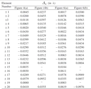
Table 2. Optimized element position perturbations ∆nfor Figs. 4(a), (b) and 6(a), (b).
n
∆
(in λ)Element
Number Figure 4(a) Figure (4b) Figure 6(a) Figure 6(b)
± 1 0.0045 0.0237 0.0017 0.0300
± 2 − 0.0200 0.0455 0.0078 0.0390
±3 − 0.0118 0.0397 − 0.0126 0.0563
± 4 − 0.0065 0.0135 − 0.0142 0.0315
± 5 − 0.0020 0.0540 − 0.0166 0.0418
± 6 − 0.0430
0.0512
0.0434
± 7 − 0.0489
0.0277
− 0.0016 0.0489
± 8 − 0.0399
0.0329
− 0.0106 0.0474
± 9 − 0.0217
0.0412
− 0.0361 0.0434
± 10 − 0.0290
0.0185
− 0.0276
± 11 − 0.0352
0.0312
− 0.0163 0.0163
± 12 − 0.0446
0.0356
0.0634
± 13 − 0.0232 0.0596 − 0.0038 0.0365
± 14 0.0030 0.0541 0.0038 0.0804
± 15 − 0.0035 − 0.0184
± 16 − 0.0030 0.0611
± 17 0.0289 0.0271 0.0578 0.0989
± 18 0.0579 0.0952 0.0355 0.0857
± 19 0.0080 0.0003
± 20 0.0410 0.0355 0.0619 − 0.0976
interference and having low SLL. Thus, the solution spaces which are the perturbation amounts of the element positions are given in Table 2, for only the Pareto optimal points pointed out in the Pareto frontiers. The radiation patterns of the points marked in Figs. 3(a) and (b) are given in Figs. 4(a) and (b), respectively. These patterns are obtained using the perturbation amounts given in Table 2. Figs. 4(a) and (b) show the results optimized by the GA in comparison with the results obtained by the uniform array and thinned array. The GA has reduced the MSLL to−13.7 dB and 5 dB suppression is achieved in the interference region for uniform array, as seen in Fig. 4(a). By using the optimized thinned array geometry the MSLL is reduced by 0.7 dB and the maximum level between 19◦–21◦ is suppressed from −22.11 dB to
−26 dB as seen in Fig. 4(b).
The main beams of the radiation patterns are directed to 75◦ for uniform array and to 80◦ for thinned array, where the maximum radiation directions are in the scanning ranges as given in Figs. 3(a) and (b). It must be noted that, the pattern features which are the MSLL and maximum level in the interference region are valid not only
(a)
(b)
0 20 40 60 80 100 120 140 160 180
-30 -25 -20 -15 -10 -5 0
theta (degree)
Normalized Gain (dB)
0 20 40 80 100 120 140 160
theta (degree) -40
-35
-30 -25 -20 -15 -10 -5 0
Normalized Gain (dB)
-40 -35
60 180
Figure 4. The radiation patterns directed to (a) 75◦, (b) 80◦ having
for the given directions, but also valid in the full prescribed range. Thus, the optimized uniform and thinned arrays can be scanned from 70◦ to 110◦ and 80◦ to 100◦, respectively.
In many cases, a broad interference may take place in the visible region of the radiation pattern or a region that the radiation pattern is not desired to be reached may exist in the visible region. For such a situation, a broad region between 15◦ and 25◦ is handled to suppress
by position perturbations in the second implementation. The same cost functions given in Eqs. (6) and (7) are used in the optimization
-12.4 -12.2 -13.8 -13.6 -13.4 -13.2 -13 -12.8 -12.6
-20
-40 -38 -36 -34 -32 -30 -28 -26 -24 -22
MSLL (dB)
max [Array Factor (15 -25 )] (dB)
(a)
-20 -19 -18 -17 -16 -15 -14 13 -27
-26 -25 -24 -23 -22 -21 -20 -19 -18
(b)
o
o
max [Array Factor (15 -25 )] (dB)
o
o
MSLL (dB) -17
process. The direction of maximum radiation is again assumed to be between the angles 40◦–140◦, 50◦–130◦, 60◦–120◦, 70◦–110◦ and 80◦–
100◦, respectively. In this example, by handling a broad region, the
suppression of the desired directions which may be corrupted because of the mutual coupling effect have been guaranteed. The Pareto frontiers for optimization of uniform and thinned arrays to achieve the desired objectives are given in Figs. 5(a) and (b).
The features of the non-optimized radiation patterns of the uniform array and the thinned array are given in Table 3, where the table the achievement of the optimization processes can be observed. For example, if a designer demands a uniform array having low SLL during scanning between 70◦–110◦ and suppressing a fixed broad
interference, he can get −13.29 dB MSLL and maximum level of
−30.18 dB with a uniform array. After the optimization for element positions of the array, a set of Pareto optimal solutions providing the same pattern features can been obtained for scanning between 60◦–120◦
without any degradation in the patern features as seen in Fig. 5(a). Furthermore, the Pareto frontier for the thinned array with the same objectives is given in Fig. 5(b). The improvement in suppressing the broad region while scanning between 60◦–120◦ can be observed using
Table 3 and Fig. 5(b). The major advantage of obtaning the Pareto frontiers is having a variety of optimal solution sets. By presenting all possible solutions flexibility of choosing the appropriate solution according to the feature demands of the radiation pattern in the design process can be supplied.
Table 3. The MSLL and the maximum level in the broad interference region of the non-optimized radiation patterns of the uniform array and the thinned array during scanning.
Uniformly Excited Thinned Excitations
MSLL max[AF(150
-250
)] MSLL max[AF(150
-250
)]
Steering between 800
-1000 −13.29 dB −31.57 d B −17.94 dB −22.08 dB
Steering between 700
-1100 −13.29 dB −30.18 d B −17.94 dB −17.94 dB
Steering between 600
-1200 −13.29 dB −27.96 dB −17.94 dB −17.94 dB
Steering between
500-1300 −13.24 dB −24. 68 dB −17.94 dB −17.94 dB Steering between
400
(a)
(b)
0 20 40 60 80 100 120 140 160 180
-30 -20 -10 0
theta (degree)
Normalized Gain (dB)
0 20 40 80 100 120 140 160
theta (degree) -40
-30 -20 -10 0
Normalized Gain (dB)
-40
60 180
Figure 6. The radiation patterns directed to (a) 50◦, (b) 65◦ having
the features of the points marked in Fig. 5(a) and (b).
The radiation patterns having the fatures of the points marked in Figs. 5(a) and (b) are given in Figs. 6(a) and (b), respectively. These patterns are composed by using the perturbation amounts given in Table 2. These figures show the results obtained from the GA in comparison with the uniform array and thinned array.
The MSLL of the radiation pattern for uniform array is reduced to
−13.8 dB with the maximum level of−33 dB in the interference region while the main beam is directed to 50◦, as seen in the Fig. 6(a). The
main beam of the radiation pattern is directed to 65◦ for thinned array
in Fig. 6(b), where the maximum radiation direction is in the scanning range given in Fig. 5(b). As Fig. 6(b) highlights, by a small amount of position perturbations of array elements, the MSLL is reduced to
−21 dB.
6. CONCLUSION
be positioned out of the scanning range in the visible region is aimed to be suppressed. The positions of uniformly excited periodic arrays and thinned arrays are optimized to achieve these objectives. The GA is used in the optimization process for obtaining all the optimal solutions. The set of optimal solutions are given by Pareto frontiers rather than giving only an optimal solution for an objective function formed by combination of weighted sums. As it is highlighted in the Pareto optimal fronts, by optimization of uniform element positions, the fixed interference region can be suppressed more successfully than thinned arrays, where the optimized thinned arrays are more capable of reducing the MSLL of the radiation patterns. Moreover, suppressing a wider interference region negatively effects the suppression success of the interference and the MSLL of the radiation pattern during scanning.
REFERENCES
1. Yan, K. K. and Y. L. Lu, “Sidelobe reduction in array pattern synthesis using genetic algorithm,”IEEE Trans. Antennas Propagat., Vol. 45, 1117–1122, 1997.
2. Bevelacqua, P. J. and C. A. Balanis, “Minimum sidelob levels for linear arrays,” IEEE Trans. Antennas Propagat., Vol. 55, 3442– 3449, 2007.
3. Khodier, M. M. and C. G. Christodoulou, “Sidelobe level and null control using particle swarm optimization,” IEEE Trans. Antennas Propagat., Vol. 53, 2674–2679, 2005.
4. Tonn, D. A. and R. Bansal, “Reduction of sidelobe levels in interrupted phased array antennas by means of a genetic algorithm,” Int. J. RF Microwave Comput. Aided. Eng., Vol. 17, 134–141, 2007.
5. Er, M. H., “Linear antenna array pattern synthesis with prescribed broad nulls,” IEEE Trans. Antennas Propagat., Vol. 38, 1496– 1498, 1990.
6. Haupt, R. L., “Phase-only adaptive nulling with a genetic algorithm,”IEEE Trans. Antennas Propagat., Vol. 45, 1009–1015, 1997.
7. Ismail, T. H. and M. M. Dawoud, “Null steering in phased arrays by controlling the element positions,” IEEE Trans. Antennas Propagat., Vol. 39, 1561–1566, 1991.
9. Mouhamadou, M., P. Armand, P. Vaudon, and M. Rammal, “In-terference suppression of the linear antenna arrays controlled by phase with use of SQP algorithm,” Progress In Electromagnetics Research, PIER 59, 251–265, 2006.
10. Guney, K. and A. Akdagli, “Null steering of linear antenna arrays using modified tabu search algorithm,” Progress In Electromagnetics Research, PIER 33, 167–182, 2001.
11. Steyskal, H., R. A. Shore, and R. L. Haupt, “Methods for null control and their effects on the radiation pattern,” IEEE Trans. Antennas Propagat., Vol. 34, 404–409, 1986.
12. Chung, Y. C. and R. L. Haupt, “Amplitude and phase adaptive nulling with a genetic algorithm,”Journal Electromagnetic Waves and Applications, Vol. 14, No. 5, 631–649, 2000.
13. Lu, Y. and B. K. Yeo, “Adaptive wide null steering for digital beamforming array with the complex coded genetic algorithm,” Proceedings of IEEE International Conference in Phased Array Systems and Technology, 557–560, Dana Point, CA, USA, 2000. 14. Ibrahim, H. M., “Null steering by real-weight control — A method
of decoupling the weights,” IEEE Trans. Antennas Propagat., Vol. 39, 1648–1650, 1991.
15. Babayigit, B., A. Akdagli, and K. Guney, “A clonal selection al-gorithm for null synthesizing of linear antenna arrays by ampli-tude control,” Journal Electromagnetic Waves and Applications, Vol. 20, No. 8, 1007–1020, 2006.
16. Lee, K. C. and J. Y. Jhang, “Application of particle swarm algorithm to the optimization of unequally spaced antenna arrays,”Journal Electromagnetic Waves and Applications, Vol. 20, No. 14, 2001–2012, 2006.
17. Hejres, J. A., “Null steering in phased arrays by controlling the positions of selected elements,”IEEE Trans. Antennas Propagat., Vol. 52, 2891–2895, 2004.
18. Kalyanmoy, D., “Multi-objective optimization using evolutionary algorithms,” John Wiley & Sons, 2001.
19. Bray, M. G., D. H. Werner, D. W. Boeringer, and D. W. Machuga, “Optimization of thinned aperiodic linear phased arrays using genetic algorithms to reduce grating lobes during scanning,”IEEE Trans. Antennas Propagat., Vol. 50, 1732–1742, 2002.
20. Haupt, R. L., “Thinned arrays using genetic algorithms,” IEEE Trans. Antennas Propagat., Vol. 42, 993–999, 1994.
22. Ares, F., J. A. Rodriguez, E. Villanueva, and S. R. Rengarajan, “Genetic algorithms in the design and optimization of antenna array patterns,” IEEE Trans. Antennas Propagat., Vol. 47, 506– 510, 1999.
23. Wolfgang, B., N. Peter, K. Robert, and F. Frank, Genetic Programming — An Introduction, Morgan Kaufmann, 1998. 24. Goldberg, D. E.,Genetic Algorithms in Search, Optimization and
Machine Learning, Kluwer Academic Publishers, 1989.