Prediction of Slot-Shape, Slot-Size and Inserted Air-Gap
of a Microstrip Antenna Using Knowledge-Based Neural Network
Taimoor Khan1, * and Asok De2
Abstract—In this paper, the slot-shape and slot-size introduced on the radiating surface of a microstrip antenna as well as the inserted air-gap between the substrate sheet and ground plane are predicted, simultaneously. This synthesizing-prediction is carried out using knowledge based neural network (KBNN) model as this approach requires very less amount of training patterns. The suggested approach is validated by fabricating and characterizing three prototypes. A very good agreement is attained in measured, simulated and predicted results.
1. INTRODUCTION
The synthesis of a microstrip antenna (MSA) deals with deriving an antenna structure, i.e., physical dimension(s) of the MSA, substrate thickness and relative permittivity [1]. Antenna synthesis is usually possible if the problem is limited to a specific type of antenna or a narrow range of specifications, and it is adequate for many applications. The synthesizing methods are valuable in guiding the antenna designers in pursuit of near optimal solutions to the problem class. The synthesis becomes more difficult for complex antenna requirements. Pattern synthesis problem, in general, is to specify pattern variables and then to determine the required antenna variable values for a given antenna geometry type [1]. To make the synthesis process easier, several simulation code packages, such as IE3D [2], HFSS [3], CST [4], and ADS [5], are developed. However, these simulators, by themselves, do not synthesize an antenna. These simulators only analyze a synthesized structure and provide calculated performance parameters. The antenna synthesis basically originates from human experience, knowledge and innovation, even though an optimum and accurate synthesis often cannot be achieved without an analysis tool. Thus, these obligations in conventional synthesis methods lead to complexities and processing cost. For fulfilling such obligations, neural networks modeling could be a better alternative [6–12]. In the last decade, artificial neural networks (ANN) modeling has acquired enormous importance in the microwave community, especially in modeling of MSAs due to their ability and adaptability features. The neural models [7–12] may not be very reliable if they are trained with small number of patterns. Also, even with sufficient training patterns, the reliability of these models is not guaranteed in extrapolation region, and in most cases, it fails. Further, the training patterns are generally created using simulation and/or measurement approach. For a complex geometry, generating large number of patterns becomes time consuming and sometimes very expensive. It is so because the simulation/measurement approach is to be performed for several combinations of input parameters.
The concept of knowledge-based neural networks (KBNN) has recently been introduced to reduce the required training patterns for a neural network in several cases [13–23]. These cases are mentioned as: designing of microwave problems [13], modeling of microwave components [14], identifying the performance of electromagnetic devices [15], modeling of stripline discontinuities [16], designing of
Received 16 January 2016, Accepted 21 March 2016, Scheduled 15 June 2016
* Corresponding author: Taimoor Khan ([email protected]).
1 Department of Electronics and Communication Engineering, National Institute of Technology, Silchar 788 010, India. 2Department
microwave phase shifters [17], modeling of microstrip T-junction [18], automatic model generating technique for microwave modeling [19], advanced electromagnetic data sampling algorithms for several microwave structures [20], reverse-modeling approach to analyze electromagnetic compatibility (EMC) of printed circuit boards (PCBs) and shielding enclosures [21], modeling for determining the data distribution, model structure adaptation, and model training in a systematic framework [22]. Hence, in [13–22], several diverse and complicated cases have been resolved using KBNN techniques, but unfortunately, the literature of KBNN techniques for modeling of microstrip antennas is very limited [23]. Watson et al. [23] have only used it for computing single performance parameter of a patch/slot antenna with co-planar waveguide (CPW) feeding. In this paper, the concept of KBNN modeling has been used for predicting slot-shape, slot-size and inserted air-gap, simultaneously. To the best of the authors’ knowledge, there is no published work for modeling such a complicated problem in the referenced literature [7–12] and [13–23]. Handling such a complicated problem using analytical/numerical techniques is still a challenging task facing the electromagnetic community. Electromagnetic simulating packages can do it roughly, but only at the cost of large computational time [3–6]. Further, the simulation approach is not suitable in the situation where instant answer is required as in the case of synthesizing microstrip antennas by antenna designers. In such adverse situations, ANN modeling is used which produces an accurate response very fast, and the concept of KBNN is incorporated for reducing required training patterns for the same required level of accuracy. The unique feature of the proposed model is to predict slot-shape, slot-size and inserted air-gap of four slotted geometries, simultaneously. These parameters are predicted for the given desired values of resonance frequencies, gains, directivities, antenna efficiencies and radiation efficiencies for dual-frequency operation. This paper is organized as follows. Section 2 describes KBNN synthesis modeling. Section 3 illustrates results and validation. Conclusion followed by references is then discussed in Section 4.
2. KBNN MODELING FOR SYNTHESIS
Neural networks are massively distributed analogous processors and becoming powerful techniques for resolving cross-disciplinary problems [6]. A neural network has usual tendency for storing empirical knowledge during training and making it available for the use during testing. The purpose of training a neural network model is to minimize the error between actual and calculated outputs. The trained model, thus obtained, is tested on some arbitrary sets of pattern which are not included during training. The algorithms for both training and testing of the neural model are implemented using the neural network tool box in MATLAB software on a personal computing machine with system configuration; Dell OptiPlex 780 Core 2 Duo CPU E8400, 3.0 GHz with 4.0 GB RAM.
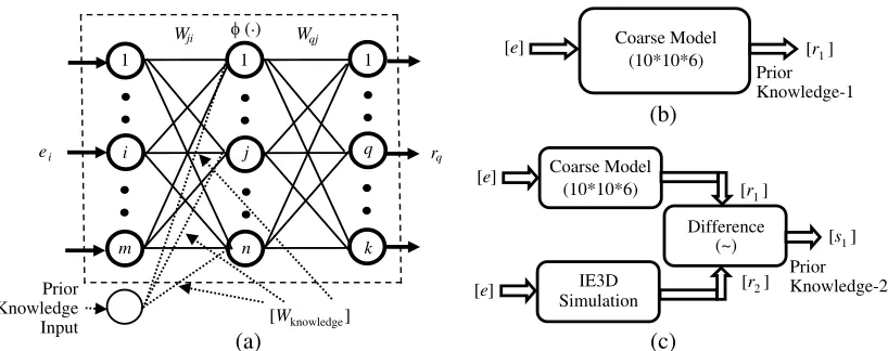
A generalized multilayered perceptron (MLP) neural model is shown in Figure 1(a), which has a structural configuration of m∗n∗k. It means that the model has m-number of neurons in the input layer,n-number of neurons in the hidden layer andk-number of neurons in the output layer. The input-to-hidden layer weights are denoted as: Wji for 1 ≤ i ≤ m and 1 ≤ j ≤ n and the hidden-to-output layer weights as: Wqj for 1 ≤ q ≤ k and 1 ≤ j ≤ n. The excitation and response of the model are represented as: eifor 1 ≤i≤mandrqfor 1≤q ≤k. The model within a box of dotted line is basically known as a MLP neural model which has extensively used in the literature [7–12]. The accuracy of this type of model depends on the number of training patterns generated by simulation/measurement, and it increases by increasing the number of training patterns. Generating a large number of training patterns is actually a time consuming process, and sometimes it becomes very expensive because the simulation/measurement approach is to be performed for several combinations of input parameters. To overcome this problem, the prior knowledge is incorporated in the existing MLP model. This prior knowledge can be attained using an analytical model, empirical model and/or an already trained neural model [23]. The attained prior knowledge is incorporated through a prior knowledge input point in the neural model shown in Figure 1(a), which is termed as a fine model for convenience. For the proposed problem, the structural configuration of this fine model is optimized as: m= 10,n= 11 andk= 6.
The prior knowledge incorporated in Figure 1(a) is attained using coarse model in two different ways illustrated in Figure 1(b) and Figure 1(c), respectively. The coarse model mentioned here is simply an MLP model shown in Figure 1(a) but with a different structural configuration (m = 10,
(a)
(b)
Prior Knowledge Input
(c)
1 1 1
i j q
m n k
i
e rq
Wji φ ( ). Wqj
[W knowledge]
[e]
[e]
[e]
[r 1]
[r 1]
[s 1]
[r 2] PriorKnowledge-2 Prior
Knowledge-1 Coarse Model
(10*10*6)
Coarse Model (10*10*6)
IE3D Simulation
Difference (~)
Figure 1. KBNN neural approach. (a) Fine model. (b) Method-1 (attained prior knowledge). (c) Method-2 (attained prior knowledge).
they are connected simultaneously, then the accuracy of the whole network is improved drastically. In Figure 1(c), the computed neural matrix [r1] is compared to its simulated counterpart matrix [r2] for
creating an error matrix [s1]. Now the matrix [r1] in Figure 1(b) and matrix [s1] in Figure 1(c) have
some prior knowledge in two different ways; one is in direct form (prior knowledge-1) whereas the other in term of error (prior knowledge-2), and thus the attained prior knowledges (prior knowledge-1 and prior knowledge-2) are applied on the Fine Model depicted in Figure 1(a), respectively. For avoiding any ambiguity, these models are denoted as KBNN model-1 which consists of Figure 1(a) + Figure 1(b) and KBNN model-2 which consists of Figure 1(a) + Figure 1(c), respectively. The training strategy of thus formed KBNN models is illustrated as follows.
Let the excitation and response matrices are as follows: [ei] where i= 1,2, . . . , m
[rq] where q= 1,2, . . . , k (1)
The weight matrices are represented as:
[wji] where j= 1,2, . . . , n and i= 1,2, . . . , m
[wqj] where q= 1,2, . . . , k and j = 1,2, . . . , n (2)
The outputs of the jth and qth neurons are:
jout = Φ (iout×wji) = Φ (ei×wji)
qout =rq = Φ (jout×wqj) (3)
The objective of the training is to reduce the global error E defined as:
E= 1
N
N
n=1
En (4)
whereN is the total number of training patterns andEnthe error corresponding tonth training pattern which is computed as follow:
En= 1 2
6
q=1
(tq−rq)2 (5)
wheretq is the target output ofqth output neuron andrq the computed output of neural model. The task of a training algorithm is to reduce this global error by adjusting the weights and biases. This is done using LM (Levenberg Marquardt) algorithm [25]. The modified weights without and with prior knowledge are mentioned in Eq. (6) and Eq. (7), respectively.
wnew(without knowledge)
= [wold]−
JTJ+μI−1JTE (6)
wnew(with knowledge)
= [wold] + [wknowledge]−
JTJ +μI−1
where J is the Jacobian matrix, and it contains basically the first derivatives of error with respect to weights and biases. The Jacobian matrix can be easily computed through a standard backpropagation algorithm [26]. In Eq. (6), I is the identity matrix whereas the combination coefficient (μ) can be predicted as reciprocal to the learning rate (η).
The training and testing patterns for the above mentioned neural approach are generated via the geometries depicted in Figure 2. The side view is shown in Figure 2(a) in which a rectangular patch of dimensions 61×56 mm2 is designed using RT-Duroid substrate RO3003 (εr = 3 and h = 0.762 mm). For getting dual-resonance, two resonating modes (TM10 and TM01) are simultaneously excited by a
single probe. An air-gap (Ag) between the substrate sheet and ground plane is then inserted [24]. The geometry after inserting an air-gap is then analyzed by inserting four different slots (viz. longitudinal-slot (LS), transverse-slot (TS), asymmetrical-cross-slot (CS) and square-slot (SS), respectively. These four slotted antennas are termed as LS-Antenna, TS-Antenna, CS-Antenna and SS-Antenna, respectively, and their top views are shown in Figure 2(b)–Figure 2(e), respectively. These geometries are analyzed using method of moments (MoM) based IE3D software [3] for creating training and testing patterns required for KBNN modeling. Different patterns for dual-resonance (f1 and f2), dual-frequency gains
(G1 andG2), dual-frequency directivities (D1 andD2), dual-frequency antenna efficiencies (A1 andA2)
and dual-frequency radiation efficiencies (R1 andR2) are generated by varying slot-dimensions (x1,y1,
x2 and y2) and thickness of air-gap (Ag), simultaneously. Thus, ten different electrical parameters (f1,
f2, G1, G2, D1, D2, A1, A2, R1 and R2) are obtained for each set of five geometrical parameters
(x1, y1, x2, y2 and Ag). These patterns are generated by varying both slot-dimensions (between
1 mm ≤slot-dimensions ≤ 50 mm) and air-gap (between 1 mm≤ air-gap≤ 10 mm). After generating the patterns, these are converted into training and testing patterns according to a statistical design of experiments (DOE) to capture the underlying input-output relationship [6]. The sampling strategy used for generating patterns is mentioned in Table 1.
After generating patterns using IE3D software, the KBNN modeling is created for predicting slot-shape (S), slot-size (x1, y1, x2 and y2) and the thickness of the inserted air-gap (Ag), simultaneously.
This prediction is carried out for achieving desired values of dual-resonance (f1 &f2), dual-frequency
gains (G1 & G2), dual-frequency directivities (D1 & D2), dual-frequency antenna efficiencies (A1 &
A2) and dual-frequency radiation efficiencies (R1 &R2). The predicted slot-shape is represented by a
dummy variable, ‘S’, where S = 1, 2, 3 and 4 corresponds to LS-Antenna, TS-Antenna, CS-Antenna and SS-Antenna, respectively.
(a) (c) TS-Antenna
Slotted Patch
Substrate
Air-Gap (A g)
Ground Plane
Patch
L L L L
x
y 1
1
x
y 1
1
x y
1 1 x
y 2
2
x
y 2
2
Feed
Patch x2 Patch Feed Patch Feed
y2 W
(b) LS-Antenna (d) CS-Antenna (e) SS-Antenna
Figure 2. Proposed slotted antennas with air-gap.
Table 1. Sampling strategy.
Parameters Specified Range Step-Size
x1 1 mm≤x1 ≤50 mm 0.1 mm
y1 1 mm≤y1≤50 mm 0.1 mm
x2 1 mm≤x2 ≤50 mm 0.1 mm
y2 1 mm≤y2≤50 mm 0.1 mm
Predictive
Synthesis
Neural Model
Slot-Shape (S) (f & f )
(G & G )
(D & D )
(A & A )
(R & R )
1 2
1 2
1 2
1 2
1 2
Slot-Size (x , y , x , y )
Air-Gap (A g)
1 2 1 2
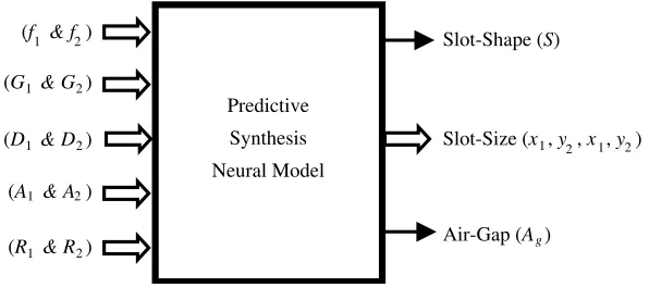
Figure 3. Predictive neural model (block-diagram).
During the training of KBNN modeling, some initial parameters, such as mean-square-error (MSE)
E = 4.8×10⁻⁵ and learning rate (η) = 0.15, are selected. Before applying training, the patterns are normalized between +0.1 to +0.9 to avoid the convergence problem of KBNN models. The initial weights and bias values are also selected as random numbers between 0 and 1. Once the training is over, the trained KBNN model then predicts the slot-shape (i.e., LS-Antenna, TS-Antenna, CS-Antenna or SS-CS-Antenna), slot-size (i.e., x1, y1, x2 and y2) and thickness of the inserted air-gap (i.e.,
Ag) within a fraction of a second for any arbitrary set of parameters: 1.5 GHz≤(f1 and f2)≤3.0 GHz,
6.2 dBi ≤(G1 and G2) ≤ 9.6 dBi, 6.6 dBi ≤ (D1 and D2) ≤9.9 dBi, 83% ≤(A1 andA2) ≤ 100% and
85% ≤ (R1 and R2) ≤100%. For better understanding of the KBNN modeling, a conventional MLP
model of structural configuration 10∗78∗76∗6 using the approach as described in the literature [7–12] is also created. The prediction of Slot-Shape (S), Slot-Size (x1,y1, x2, y2) and inserted Air-Gap (Ag)
is summarized using block-diagram in Figure 3. The excitation for the block-diagram is mentioned as: dual-resonance (f1 &f2), dual-frequency gains (G1 & G2), dual-frequency directivities (D1 &D2),
dual-frequency antenna efficiencies (A1 & A2) and dual-frequency radiation efficiencies (R1 & R2),
simultaneously.
3. RESULTS AND VALIDATION 3.1. Numerical Results
In this paper, a conventional MLP model along with two KBNN models (KBNN model-1 and KBNN model-2) are proposed for predicting slot-shape, slot-size and inserted air-gap of four different geometries, simultaneously. Table 2 illustrates a comparison of optimized values of weights and biases in three neural models. These optimized values are calculated using Equation (8). It is clear from Table 2 that the optimized weights and biases in KBNN models are less than that of MLP model. Thus, in KBNN models, the optimized weights and biases are reduced by 96.62% and 79.38%. It means that the KBNN models require only 3.38% weights and 20.62% bias values of that of MLP model.
Total Optimized Weights = (10×76) + (76×78) + (78×6) = 7156
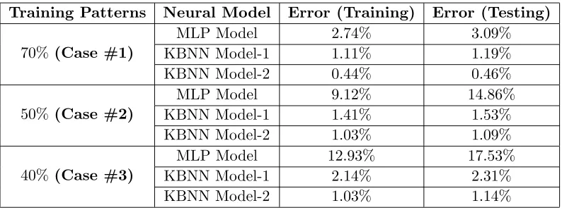
and Total Optimized Biases = (76 + 78 + 6) = 160 (8) Table 3 shows an accuracy comparison in three neural models. In computing the accuracy, three different cases, Case #1, Case #2 and Case #3 having 70%, 50% and 40% training patterns, are
Table 2. Comparison of weights and biases.
Neural Model Optimized Structure Optimized Weights Optimized Biases
MLP Model 10∗76∗78∗6 7156 160
KBNN Model-1 10∗10∗6 and 16∗11∗6
242 33
considered. It is clear from Table 3 that the percentage error in MLP model is drastically increased by reducing the training patterns from 70% to 40%. It means that the MLP model produces accurate results only if it is trained with adequate number of training patterns. On the other hand, both the KBNN models produce more accurate results even with lower number of training patterns. During testing of KBNN model-1, the accuracy is changed from 1.19% to 2.31% by reducing the number of training patterns from 70% to 40%, whereas in KBNN model-2, it is changed from 0.46% to 1.14% only for the same level of reduction in training patterns. Thus, KBNN model-2 is observed more accurate than KBNN model-1 for the proposed problem.
Table 3. Accuracy comparison in neural models.
Training Patterns Neural Model Error (Training) Error (Testing)
70%(Case #1)
MLP Model 2.74% 3.09%
KBNN Model-1 1.11% 1.19%
KBNN Model-2 0.44% 0.46%
50%(Case #2)
MLP Model 9.12% 14.86%
KBNN Model-1 1.41% 1.53%
KBNN Model-2 1.03% 1.09%
40%(Case #3)
MLP Model 12.93% 17.53%
KBNN Model-1 2.14% 2.31%
KBNN Model-2 1.03% 1.14%
For initialization purpose, the weight and bias values are randomly selected between 0 and 1. Thus, to observe the overall behavior of computed errors, the stochastic behavior of the mean and standard deviation of computed errors are analyzed. For this purpose, a relationship between mean and standard deviation (SD) is developed by considering a term coefficient of variation (CoV) which is defined as the ratio of standard deviation (SD) to the mean value. CoV closer to 0 represents greater uniformity whereas CoV closer to 1 represents larger variability of the errors [27]. For KBNN model-2, the mean and standard deviation of five-dimensional computed error are mentioned as follow:
[Mean] = [1.4412 1.4142 1.4366 1.4227 1.3952] and
[SD] = [0.1505 0.1486 0.1483 0.1517 0.1539]
(9)
Hence, the coefficient of variation (CoV) is computed as:
[CoV] = SD
Mean = [0.1044 0.1051 0.1032 0.1066 0.1103] (10) Thus, the overall error points are uniformly distributed over a full validation set of simulated patterns as the computed CoV matrix is closer to 0 which further supports the effectiveness of KBNN model-2. Same order of error distribution is achieved in KBNN model-1 too.
During simulating a structure in IE3D software, 1.5 GHz to 3.0 GHz frequency range with total 100-sampling points is used. The simulation time in IE3D software depends on the complexity inserted in the geometry. For the proposed structures, it is roughly computed as ∼1 hr 53 min/structure. By using neural modeling, the computational time is fairly reduced. Using LM algorithm, the MLP model is trained in 1633 sec. (∼27 min) and requires 29651 iterations. The time elapsed during testing of the neural models is computed using MATLAB syntax ‘cputime’ as mentioned below:
Start of Testing Algorithm
Program Statement-1
Program Statement-2
. . . .
End of Testing Algorithm
Time Elapsed = cputime-time 1
=∼44 msec. for MLP model (or ∼31 msec. KBNN model-2)
This procedure is repeated for several independent runs, and finally it is concluded that the MLP model and KBNN model require ∼44 msec and ∼31 msec, respectively in producing the results after training [25]. Thus, these neural models after training are much faster than that of the simulation method.
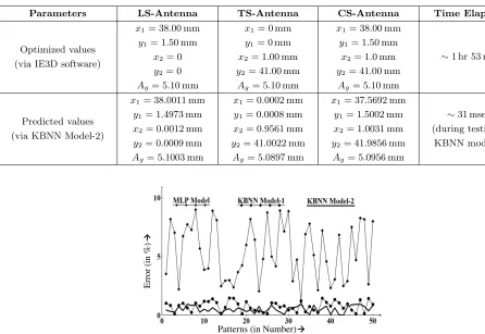
Also the training of the MLP model requires only ∼ 27 kB system RAM, and for testing the performance, only ∼1.44 kB RAM is required. Hence, the required memory space in both training and testing of MLP model is also less than 36 MB required for simulation. The structural configuration (i.e., number of hidden layers as well as neurons in each hidden layer) of two KBNN models is less than that of MLP model. Hence, the KBNN models require less memory space than that of the MLP model. The optimized values via IE3D software and predicted values via KBNN model-2 are also compared, and this comparison is illustrated in Table 4 which shows a very good agreement between the two.
The three neural modeling schemes are also tested in the extrapolation region (i.e., outside the region of training patterns) by expanding the original input space by 25%. By doing this, total 50 arbitrary sets of pattern are created for each slotted antenna geometry. The percentage errors in
Table 4. Comparison of simulated and predicted values.
Parameters LS-Antenna TS-Antenna CS-Antenna Time Elapsed
Optimized values (via IE3D software)
x1= 38.00 mm
y1= 1.50 mm
x2= 0 y2= 0
Ag= 5.10 mm
x1= 0 mm
y1= 0 mm
x2= 1.00 mm
y2= 41.00 mm
Ag= 5.10 mm
x1= 38.00 mm
y1= 1.50 mm
x2= 1.0 mm
y2= 41.00 mm
Ag= 5.10 mm
∼1 hr 53 min
Predicted values (via KBNN Model-2)
x1= 38.0011 mm
y1= 1.4973 mm
x2 = 0.0012 mm
y2= 0.0009 mm
Ag= 5.1003 mm
x1= 0.0002 mm
y1= 0.0008 mm
x2= 0.9561 mm
y2= 41.0022 mm
Ag= 5.0897 mm
x1= 37.5692 mm
y1= 1.5002 mm
x2= 1.0031 mm
y2= 41.9856 mm
Ag= 5.0956 mm
∼31 msec.
(during testing of KBNN model-2)
Patterns (in Number)
Error (in %)
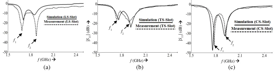
Table 5. Comparison of dual-resonances (f1 &f2) in GHz.
LS-Antenna TS-Antenna CS-Antenna
Measured Values
Simulated Values
Measured Values
Simulated Values
Measured Values
Simulated Values
1.6850 & 1.8750 1.7020 & 1.8430 1.7420 & 1.8940 1.7630 & 1.9140 1.7800 & 1.9250 1.7630 & 1.9140
computed parameters are then compared, and it is concluded that the accuracy of KBNN models is slightly depreciated for all 50 generated patterns compared to that of MLP model. It may be due to built-in prior knowledge in the KBNN models to give more information to the patterns not seen during the training. Figure 4 summarizes the extrapolation capability of three neural models in predicting the inserted air-gap (Ag) of Antenna-3. The same level of accuracy is observed in predicting the slot-size too.
3.2. Experimental Results
For validating the proposed work, three prototypes, corresponding to LS-Antenna, TS-Antenna and CS-Antenna, are also fabricated using RT-Duroid substrates, respectively. The slotted rectangular patch is etched on upper side of the substrate, whereas an air-gap of 5.1 mm is inserted between substrate and ground plane using Teflon rods as shown in Figure 5(a). The top views for these three prototypes are shown in Figure 5(b), Figure 5(c) and Figure 5(d), respectively.
Figure 6 compares the measured and simulated values of S-parameters. A good convergence between them confirms that the Teflon rods do not affect antenna performance. Further, during measurement, the bandwidth of the CS-Antenna is measured as: 55.50 MHz, whereas during simulation it has been observed as 250 MHz (1.99 GHz–1.74 GHz). It may be due to lack of caution in fabricating and/or inserting the air-gap using Teflon rods. Furthermore, the size and losses of the solder joints are not considered during the simulation which may also cause this difference. Further, Table 5 illustrates a comparison of measured and simulated dual-resonances for three slotted antennas which also shows a very good conformity.
(a) (b)
Teflon Rods
SMA Connector 5.1 mm Air-Gap
(ii) TS-Antenna
(i) LS-Antenna (ii) CS-Antenna
Figure 5. Slotted antennas with inserted air-gap (screen-shots). (a) Side-view. (b) Top-view.
(a) (b) (c)
f (GHz) f (GHz) f (GHz)
|
S
| (dB)
11
|
S
| (dB)
11
|
S
| (dB)
11
f f 1
2
f f 1
2
f f
1 2
(a) (b) (c)
Angle (Deg.)
Amplitude (dB)
Angle (Deg.) Angle (Deg.)
Amplitude (dB) Amplitude (dB)
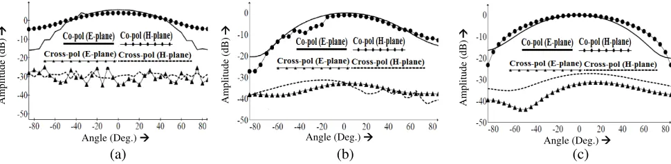
Figure 7. Co- and cross-polarizations (measured values). (a) Patterns at 1.6850 GHz (LS-Antenna). (b) Patterns at 1.7420 GHz (TS-Antenna). (c) Patterns at 1.7800 GHz (CS-Antenna).
The dual-resonance of the referenced patch antenna without any slot is obtained as: 2.0256 GHz and 2.1970 GHz. The measured and simulated dual-resonances of slotted antennas are summarized in Table 5. Hence, by inserting a slot, the excited surface current path lengthens, increasing the antenna length and hence decreasing the dual-resonance. Thus, the dual-resonance is lowered in three slotted prototypes showing their fair compactness.
The normalized radiation patterns for both E- and H-planes are also measured. For the first resonance, these patterns are shown in Figure 7(a), Figure 7(b) and Figure 7(c), respectively. Figure 6 shows that the ratio of co-to-cross polarizations is higher than 30 dB inE-plane and higher than 20 dB inH-plane. The same degree of co-to-cross polarization ratio is achieved for the second resonance too.
4. CONCLUSION
In this paper, an MLP neural model has been suggested for synthesizing four slotted microstrip antennas with inserted air-gap, simultaneously. The MLP model has been used for instantly predicting slot-shape, slot-size and thickness of inserted air-gap, simultaneously. The neural model for such a complicated case has been rarely attempted earlier in the open literature. For MLP model, the level of convergence is ≤ 3% as mentioned in Table 3. Two knowledge-based neural models have also been proposed for reducing the required number of training patterns. These models have shown better accuracy even with less number of training patterns, for both interpolation and extrapolation regions. Thus, the knowledge-based neural approach can be helpful for the antenna designers in a situation where the generation of patterns is expensive and time-consuming.
In general, a neural implementation of four different slotted microstrip antennas may require four different neural modules, but in the proposed work, one module can fulfill the requirement of four different neural modules. Thus, the present approach may be considered as a generalized approach in this sense. Hence, the proposed approach can be helpful for the design engineers in prediction of the slot-shape, slot-size and the amount of inserted air-gap, simultaneously for the desired level of performance parameters.
REFERENCES
1. Bahl, I. J. and P. Bhartia, Microstrip Antennas, Artech House, Dedham, Mass, 1981. 2. IE3D, Zeland Software Inc., Fremont, CA.
3. Ansoft Corporation, HFSS Simulation Tool.
4. CST GmbH-Computer Simulation Technology, CST Microwave Studio. 5. Agilent Technologies, ADS Simulator.
7. Wang, Z., S. Fang, Q. Wang, and H. Liu, “An ANN-based synthesis model for the single-feed circularly-polarized square microstrip antenna with truncated corners,”IEEE Trans. on Antennas Propag., Vol. 60, 5989–5992, 2012.
8. Aneesh, M., J. A. Ansari, A. S. Kamakshi, and S. S. Sayeed, “Investigations for performance improvement of X shaped RMSA using artificial neural network by predicting slot size,” Progress In Electromagnetics Research C, Vol. 47, 55–63, 2014.
9. Wang, Z. and S. Fang, “ANN synthesis model of single-feed corner-truncated circularly polarized microstrip antenna with an air-gap for wideband applications,”International Journal of Antennas and Propagation, 7 pages, Article ID 392843, Hindawi Publishing Corporation, 2014.
10. Can, S., K. Y. Kapusuz, and E. Aydin, “Calculation of resonant frequencies of a shorting PIN-loaded ETMA with ANN,” Microwave Opt. Technol. Lett., Vol. 56, 660–663, 2014.
11. Bedra, S. and R. Bedra, “Radiation characteristics of circular microstrip patch antenna with and without air-gap using neuro-spectral computation approach,” WSEAS Transactions on Communications, Vol. 13, 340–347, 2014.
12. Gunavathi, N. and D. Sriram Kumar, “Estimation of resonant frequency and bandwidth of compact unilateral coplanar waveguide-fed flag shaped monopole antennas using artificial neural network,”
Microwave Opt. Technol. Lett., Vol. 57, 337–342, 2015.
13. Wang, F. and Q. J. Zhang, “Knowledge-based neural models for microwave design,”IEEE Trans. Microw. Theory and Techniques, Vol. 45, No. 12, 2333–2343, 1997.
14. Watson, P. M., K. C. Gupta, and R. L. Mahajan, “Applications of knowledge-based artificial neural network modeling to microwave components,” Int. J. RF and Microwave CAE, Vol. 9, 254–260, 1999.
15. Frederic, D. and A. L. Devid, “Electromagnetic device performance identification using knowledge based neural networks,” IEEE Trans. on Magnetics, Vol. 35, No. 3, 1817–1820, 1999.
16. Wang, B.-Z., D. Zhao, and J. Hong, “Modeling stripline discontinuities by neural network with knowledge-based neurons,”IEEE Trans. Advanced Packaging, Vol. 23, No. 4, 692–698, 2000. 17. Reto, Z. and K. C. Gupta, “An approach for knowledge-aided-design (KAD) of microwave circuits
using artificial neural networks,” IEEE MTT Digest, 1011–1014, 2001.
18. Hong, J. and B.-Z. Wang, “NNKBN model for the microstrip T-junction structure,”International Symposium Antennas and Propagation Society, Vol. 2, 92–95, Columbus, USA, 2003.
19. Devabhaktuni, V. K., B. Chattaraj, M. C. E. Yagoub, and Q. J. Zhang, “Advanced microwave modeling framework exploiting automatic model generation knowledge neural networks, and space mapping,”IEEE Trans. Microw. Theory and Techniques, Vol. 51, No. 7, 1822–1833, 2003.
20. Rayas-Sanchez, J. E. and Q. J. Zhang, “On knowledge-based neural networks and neuro-space mapping,” IEEE MTT-S International Montreal Microwave Symposium Digest (MTT), 1–3, 17– 22, Canada, 2012.
21. Devabhaktuni, V., C. F. Bunting, D. Green, D. Kvale, L. Mareddy, and V. Rajamani, “A new ANN-based modeling approach for rapid EMI/EMC analysis of PCB and shielding enclosures,”
IEEE Trans. Electromagnetic Compatibility, Vol. 55, 385–394, 2013.
22. Na, W. C. and Q. J. Zhang, “Automated knowledge-based neural network modeling for microwave applications,” IEEE Microwave and Wireless Components Letters, Vol. 24, No. 7, 499–501, 2014. 23. Watson, P. M., G. L. Creech, and K. C. Gupta, “Knowledge based EMANN models for the design
of wide bandwidth CPW patch/slot antennas,” IEEE International Symposium on Antennas and Propagation Society, Vol. 4, 2588–2591, 1999.
24. Dahele, J. S. and K. F. Lee, “Theory and experiment on microstrip antennas with air-gaps,” IEE Proc., Vol. 132, No. 7, 455–460, 1985.
25. Higham, D. J. and N. J. Higham, MATLAB Guide, SIAM, PA, 2005.
26. Hagan, M. T. and M. B. Menhaj, “Training feed forward networks with the Marquardt algorithms,”
IEEE Trans. Neural Networks, Vol. 5, 989–993, 1995.
27. Freni, A., M. Mussetta, and P. Pirinoli, “Neural network characterization of reflectarray antennas,”