Copyright2001 by the Genetics Society of America
Parallel Computation of a Maximum-Likelihood Estimator of a Physical Map
Suchendra M. Bhandarkar,* Salem A. Machaka,* Sanjay S. Shete
†and Raghuram N. Kota*
*Department of Computer Science,†Department of Statistics, The University of Georgia, Athens, Georgia 30602-7404 Manuscript received September 1, 2000
Accepted for publication December 19, 2000
ABSTRACT
Reconstructing a physical map of a chromosome from a genomic library presents a central computational problem in genetics. Physical map reconstruction in the presence of errors is a problem of high computa-tional complexity that provides the motivation for parallel computing. Parallelization strategies for a maximum-likelihood estimation-based approach to physical map reconstruction are presented. The estima-tion procedure entails a gradient descent search for determining the optimal spacings between probes for a given probe ordering. The optimal probe ordering is determined using a stochastic optimization algorithm such as simulated annealing or microcanonical annealing. A two-level parallelization strategy is proposed wherein the gradient descent search is parallelized at the lower level and the stochastic optimization algorithm is simultaneously parallelized at the higher level. Implementation and experimental results on a distributed-memory multiprocessor cluster running the parallel virtual machine (PVM) envi-ronment are presented using simulated and real hybridization data.
G
ENERATION of entire chromosomal maps has netic map of the same chromosome, i.e., 10–100 kb (Brodyet al.1991). Physical maps have provided funda-been a central problem in genetics right from itsearly years (Sturtevant1913). These maps are central mental insights into gene development, gene organiza-tion, chromosome structure, recombinaorganiza-tion, and the to the understanding of the structure of genes, their
function, their transmission, and their evolution. Recent role of sex in evolution and have also provided a means for the recovery and direct molecular manipulation of advances in molecular genetics have led to a wealth of
DNA markers along a chromosome and also eased the genes of interest (Pradeet al.1997).
Several techniques exist for generation of physical process by which these markers can be assayed.
Conse-quently, the focus of current research has shifted from maps from contig libraries. These techniques are spe-cific to an experimental protocol and the type of data data collection to the computational problem of map
collected, for example, mapping by nonunique probes assembly.
(Alizadehet al.1995), mapping by unique probes (Ali-Chromosomal maps fall into two broad categories—
zadehet al. 1994;GreenbergandIstrail 1995;Jain
genetic mapsandphysical maps.Genetic maps represent
and Myers 1997), mapping by unique endprobes an ordering of genetic markers along a chromosome
(Christofet al.1997), mapping using restriction frag-where the distance between two genetic markers is
re-ments (Fasuloet al.1997;JiangandKarp1997), map-lated to their recombination frequency. Genetic maps
ping using radiation-hybrid data (Ben-DorandChor are typically of low resolution, i.e., 1–10 Mb (Lander
1997;Slonimet al.1997), and optical mapping (Muthu-andGreen1987). While genetic maps enable a scientist
krishnan and Parida 1997; Karp and Shamir 1998; to narrow the search for genes to a particular
chromo-Lee et al. 1998). Likewise, several computation
tech-somal region, it is a physical map that ultimately allows
niques based on deterministic optimization and stochas-the recovery and molecular manipulation of genes of
tic optimization have been reported in the literature in interest. A physical map is defined as an ordering of
the context of physical mapping. Examples of stochastic distinguishable (i.e., sequenced) DNA fragments called
optimization algorithms include simulated annealing
clonesorcontigsby their position along the entire
chro-(Cuticchiaet al.1992, 1993;Mottet al.1993; Aliza-mosome where the clones may or may not contain
ge-dehet al.1994, 1995) and the random cost algorithm
netic markers. The physical mapping problem is
there-(Wanget al.1994a) whereas those of deterministic opti-fore one of reconstructing the order of clones and
mization algorithms include linear programming (Jain determining their position along the chromosome. A
andMyers 1997), integer programming (Christofet
physical map has a much higher resolution than a
ge-al.1997), integer linear programming with polyhedral combinatorics (ChristofandKececioglu1999), and semidefinite programming (Chor and Sudan 1995). Corresponding author:Suchendra M. Bhandarkar, Department of Various statistical analyses of the aforementioned physi-Computer Science, The University of Georgia, 415 Boyd Graduate
cal mapping techniques have also been reported in the
Studies Research Ctr., Athens, GA 30602-7404.
E-mail: [email protected] literature (LanderandWaterman1988;Arratiaet al.
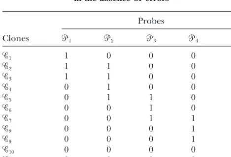
Figure 1.—An example of clone-probe ordering along a chromosome.
1991;Zhang andMarr1993;Balding1994;Nelson ᏼandHij⫽0 otherwise. Table 1 shows the clone-probe
hybridization data in the absence of errors resulting andSpeed1994;Xionget al.1996;Wilsonet al.1997).
The physical mapping protocol:The physical mapping from the example depicted in Figure 1. If the probes inᏼwere ordered with respect to their position along protocol essentially determines the nature of clonal data
and the probe selection procedure. The physical map- a chromosome, then by selecting from Ha common overlapping clone for each pair of adjacent probes in ping protocol adhered to in this project is the one based
on sampling without replacement (Fu et al. 1992). This ᏼa minimal set of clones and probes that covers the
entire chromosome (i.e., a minimal tiling) could be protocol has been used successfully in physical mapping
of Aspergillus nidulans(Brody et al. 1991;Prade et al. obtained. Note that a common overlapping clone
be-tween two adjacent probes would hybridize to both 1997),Schizosaccharomyces pombe(Mizukamiet al.1993),
probes. The minimal tiling in conjunction with the
se-and Pneumocystis carinii (Arnold andCushion 1997)
quencing of each individual clone/probe in the tiling and is currently being used in physical mapping projects
and a sequence assembly procedure that determines the
of A. flavus and Neurospora crassa (Aign et al. 2001;
overlaps between successive sequenced clones/probes Kelkaret al.2001) under the Fungal Genome Initiative
in the tiling (KececiogluandMyers1995) could then (Arnold1997;Bennett 1997).
be used to reconstruct the DNA sequence of the entire The protocol that generates the probe setᏼand the
chromosome. clone set Ꮿ is an iterative procedure that can be
de-In reality, the hybridization experiments are rarely scribed as follows. Let Ꮿi andᏼi be the clone set and
error free. The hybridization matrix H could be ex-the probe set, respectively, at ex-theith iteration. The initial
pected to contain false positives and false negatives. The clone set Ꮿ0 consists of all the clones in the library
matrix element Hijwould be a false positive if Hij ⫽ 1
whereas the initial probe set ᏼ0 ⫽ φ. The clones in
(denoting hybridization of the ith clone with the jth Ꮿ0 are designed to be of the same length and to be
probe) when in factHij⫽0. Conversely,Hijwould be a
overlapping so that each clone samples a fragment of
false negative if Hij ⫽ 0 when in fact Hij ⫽ 1. Other
the chromosome and the coverage of the entire
chromo-sources of error include chimerism wherein a single some is made possible. At the ith iteration a clonec is
clone samples two or more distinct regions of a chromo-chosen at random fromᏯiand added toᏼi. Clonecis
some, deletions wherein certain regions of the chromo-hybridized to all the clones inᏯi. The subset of clones
some are not sampled during the cloning process, and Ꮿcthat hybridize to clonecare removed fromᏯiso that
repeats wherein a clone samples a region of the chromo-Ꮿi⫹1⫽Ꮿi⫺Ꮿc. Note thatc苸Ꮿcsince a clone hybridizes
some with repetitive DNA structure. In this article, we to itself. The hybridization experiment entails
ex-tracting complementary DNA from both ends of a probe, washing the DNA over the arrayed plate, and
TABLE 1
recording all clones in the library to which the DNA
sticks (i.e., hybridizes). The above procedure is halted An example of clone-probe hybridization data in the absence of errors
at thekth iteration whenᏯk⫽φ. The final probe set is
given byᏼ⫽ ᏼk
and the clone set byᏯ⫽Ꮿ0⫺ᏼk
. In
Probes the absence of errors, the probe set ᏼ represents a
maximal nonoverlapping subset of Ꮿ0 since any clone
Clones ᏼ1 ᏼ2 ᏼ3 ᏼ4 ᏼ5
that overlaps with a given probe would hybridize to
Ꮿ1 1 0 0 0 0
one end of that probe and be effectively removed from
Ꮿ2 1 1 0 0 0
consideration in future iterations of the aforemen- Ꮿ
3 1 1 0 0 0
tioned iterative procedure. Figure 1 depicts the probes Ꮿ
4 0 1 0 0 0
and clones along the length of a chromosome where Ꮿ5 0 1 1 0 0 the clones and probes are numbered from left to right. Ꮿ6 0 0 1 0 0
Ꮿ7 0 0 1 1 0
The clone-probe overlap pattern is represented in the
Ꮿ8 0 0 0 1 0
form of a binary hybridization matrixHwhere the
ma-Ꮿ9 0 0 0 1 1
trix element Hij denotes the hybridization of the ith Ꮿ
10 0 0 0 0 1
clone苸 Ꮿto thejth probe苸ᏼ. The matrix element Ꮿ
11 0 0 0 0 1
confine ourselves to errors in the form of false positives ordering ⌸ ⫽(1,2, . . . , n) of the probes and also
the correct spacingY⫽ (Y1,Y2, . . . ,Yn)between the and false negatives. Since the clones (and probes) in the
mapping projects that use the aforementioned protocol probes. The ordering ⌸ is a permutation of (1, . . . ,n) that gives the labels (indices) of the probes
are generated using cosmids, which makes them
suffi-ciently small (ⵑ40 kb), chimerism and deletions do not in left-to-right order across the chromosome. In the interprobe spacing vectorY,Y1 denotes the space be-pose a serious problem. However, repeats do be-pose a
problem but are not explicitly addressed here; rather tween the left end of the first probe P1 and the left
end of the chromosome, and Yi the spacing between
they are treated as multiple isolated incidences of false
positives. the right end of probePi⫺1and the left end of probe Pi(where 2 ⱕi ⱕ n). The spacing between the right In this article we present a maximum-likelihood (ML)
estimator (Shete 1998; Kececioglu et al. 2000) that end of probePnand the right end of the chromosome is given byYn⫹1⫽N ⫺nM⫺ Rni⫽1 Yi, whereNis length
determines the ordering of probes in the probe setᏼ
and the interprobe spacings under a probabilistic model of the chromosome andMis the length of each clone/ probe. Note that our protocol requires that all probes of hybridization errors consisting of false positives and
false negatives. The estimation procedure involves a and clones be of the same length.
The problem as stated above is ill posed in the precise combination of discrete and continuous optimization,
where determining the probe ordering entails discrete sense as defined by Hadamard (1923). A problem is deemed well posed when its solution exists and is (i.e., combinatorial) optimization, whereas determining
the interprobe spacings for a particular probe ordering unique. A problem is ill posed when no solution exists or, if a solution does exist, it is not unique. In our case, entails continuous optimization. We propose a two-level
parallelization strategy for efficient implementation of the problem is ill posed since the underlying constraints do not imply a unique solution. Any probe ordering⌸ the above estimator. The upper level consists of parallel
discrete optimization using simulated annealing or mi- and any interprobe spacing vector Y that satisfies the requirements that Yi ⱖ0; 1ⱕ iⱕn and N ⫺nM⫺
crocanonical annealing whereas the lower level consists of the parallel conjugate gradient descent procedure. Rn
i⫽1Yiⱖ 0, constitute a valid solution. Hence the
prob-lem is formulated as one of determining a probe order-The resulting parallel algorithms are implemented on
a distributed-memory multiprocessor cluster using the ing and the interprobe spacings that maximize the likeli-hood of the observed hybridization matrix H given parallel virtual machine (PVM) environment
(Sunde-ram 1990;Geist et al. 1994). Convergence, speed-up, predefined probabilities for false positives and false neg-atives.
and scalability characteristics of the parallel algorithms
are examined and discussed. Mathematical notation: The mathematical notation used in the formulation of the maximum-likelihood esti-mator is given below:
MATERIALS AND METHODS
N, length of the chromosome; Cosmid libraries used to construct the physical map ofN.
M, length of a clone/probe; crassadiscussed in this article are described inKelkaret al.
n, number of probes; (2001). The physical mapping data were generated by DNA
hybridization described inKelkaret al.(2001). Assignments k, number of clones;
of markers to physical and genetic maps was achieved by com- , probability of false positive; plementation, hybridization, and cosmid end sequencing as , probability of false negative; described inKelkaret al.(2001).
H⫽((hi,j))1ⱕiⱕk, 1ⱕjⱕn; clone-probe hybridization matrix,
where MATHEMATICAL FORMULATION
OF THE ML ESTIMATOR h
i,j⫽
1 if cloneᏯihybridizes with probeᏼj
0 otherwise; In this section we present a brief synopsis of the ML
estimator proposed in Kececioglu et al. (2000) and Hi,ith row of the hybridization matrix;
⌸ ⫽ (1, . . . , n), permutation of {1, 2, . . . , n},
Shete(1998). The estimator reconstructs the ordering
of probes in the probe setᏼand the interprobe spacings which denotes the probe labels in the ordering when scanned from left to right along the chromosome; under a probabilistic model of hybridization errors
con-sisting of false positives and false negatives. pi⫽Rnj⫽1hij, number of 1’s inHi;
P⫽Rk
i⫽1pi, total number of 1’s inH,Y⫽(Y1,Y2, . . . ,
The probe ordering problem can be formally stated
as follows. Given a setᏼ⫽{P1,P2, . . . ,Pn} ofnprobes Yn), vector of interclone spacings, whereYiis the
spac-ing between the right end of Pi⫺1 and the left end
and a setᏯ⫽{C1,C2, . . . ,Ck} ofkclones generated using
the sampling-without-replacement protocol described ofPi(2ⱕiⱕn), andY1is the spacing between the left end of P1and the left end of the chromosome;
earlier and thek⫻nclone-probe hybridization matrix
H containing both false positives and false negatives and
Ᏺ債n, set of feasible interprobe spacingsY⫽{Y1, . . . ,
Figure 2.—Interprobe spacings: Case 1.
Yn} such thatYiⱖ 0, 1ⱕi ⱕn, andN ⫺nM ⫺Rni⫽1 Length of the Both region between probes Pj and
Yiⱖ0. P
j⫹1
The model:Given a vector of interprobe spacingsY⫽
(Y1, . . . ,Yn), there are 2n⫹1possible cases to consider ⫽
0 ifYj⫹1⬎ M
M⫺Yj⫹1 ifYj⫹1ⱕ M
depending on whether 0 ⱕ Yi ⱕ Mor Yi⬎ M, where
0ⱕ i ⱕ n ⫹ 1. Without loss of generality, we present ⫽ M⫺min(Yj⫹1,M), (1) the maximum-likelihood model forn⫽3 and illustrate
and forj⫽1, . . . ,n, 3 of the 24⫽16 possible cases.
Case 1:0ⱕ Y1 ⱕM, 0ⱕY2ⱕ M, 0ⱕ Y3 ⱕM, and Length of the
Onlyregion of probePj
0ⱕY4ⱕMas depicted in Figure 2.
Case 2:0ⱕ Y1 ⱕM, 0ⱕY2ⱕ M, 0ⱕ Y3 ⱕM, and
Y4⬎Mas depicted in Figure 3.
Case 3:Y1⬎ M, 0ⱕ Y2 ⱕM, 0ⱕ Y3ⱕ M, and 0ⱕ
Y4ⱕMas depicted in Figure 4. ⫽
Yj⫹Yj⫹1 ifYjⱕMandYj⫹1 ⱕM
M⫹Yj ifYj⬎MandYj⫹1ⱕ M
Yj⫹ M ifYjⱕMandYj⫹1⬎ M 2M ifYj⬎MandYj⫹1 ⬎M In Case 1 above, if the left end of a clone falls in
regions A, C, or E, then the clone will hybridize only withP1,P2, orP3, respectively (Figure 2). Similarly, if
⫽min(Yj,M)⫹ min(Yj⫹1,M), (2) the left end of a clone falls in region B or D, then the
clone will hybridize with both P1 and P2 or P2 and and forj⫽0, . . . ,n, P3, respectively (Figure 2). In Case 2 above, if the left
end of a clone falls in region E, then the clone will Length of theNoneregion after probe Pj
hybridize with onlyP3and if it falls in region F, then
the clone will not hybridize with any of the probes
(Fig-⫽
Yj⫹1⫺ M ifYj⫹1⬎ M
0 ifYj⫹1ⱕ M ure 3). Similarly, in Case 3 above, if the left end of a
clone falls in region A, the clone will not hybridize with
⫽Yj⫹1⫺ min(Yj⫹1,M). (3)
any of the probes (Figure 4). Therefore, from the above three cases it is easy to see that, in general, there will
We assume that the left ends of the clones are uniformly be three different types of regions, namely,
distributed over the interval [0,N⫺M];i.e., the probes are uniformly distributed across the length of the chro-Type 1:Bothregion between probePjandPj⫹1, forj⫽
mosome. Therefore it can be shown that forj⫽1, . . . , 1, . . . , n ⫺ 1. An intervening clone hybridizes to
n⫺1, the probabilityPBoththat a randomly chosen clone both probes if its left end falls in this region.
will fall in theBothregion of probesPjandPj⫹1is given
Type 2: Onlyregion of probe Pj, forj ⫽1, . . . ,n.A
by clone will hybridize to Pjonly if its left end falls in
this region.
Type 3:None region after probePj, forj⫽ 0, . . . ,n. PBoth⫽
M ⫺min(Yj⫹1,M)
N ⫺M ; (4)
A clone will hybridize to no probe if its left end falls
in this region. Here probe P0 is referred to as the for j⫽1, . . . , n the probabilityP
Onlythat a randomly beginning of the chromosome.
chosen clone will fall in theOnlyregion of probePjis
given by It can be shown that forj⫽1, . . . ,n⫺1,
POnly⫽
min(Yj,M)⫹ min(Yj⫹1,M)
N⫺M , (5) hi,j⫹1⫽
0 with probability
1 with probability (1⫺ ), (12)
and forj⫽0, . . . ,nthe probabilityPNonethat a randomly and fork⫽1, . . . ,n, wherek⬆j,j⫹1, chosen clone will fall in the None region after probe
Pjis given by hi,
k⫽
0 with probability (1⫺ )
1 with probability. (13)
PNone⫽
Yj⫹1⫺ min(Yj⫹1,M)
N⫺ M . (6) Hence,
P(Hi|⌸,Y,Bi,j)⫽(1⫺ )(hi,j⫹hi,j⫹1)·(2⫺hi,j⫺hi,j⫹1)
The conditional probability of observing a clonal
sig-natureHi (i.e., the ith row in the hybridization matrix ·(pi⫺hi,j⫺hi,j⫹1)· (1⫺ )(n⫺2)⫺(pi⫺hi,j⫺hi,j⫹1). H), given a probe ordering⌸and an interprobe spacing
(14) vectorY, is given by
Finally, for a given probe ordering⌸and interprobe
P(Hi| ⌸,Y)⫽
兺
n
j⫹1
P(Hi |⌸,Y,Oi,j)P(Oi,j|⌸,Y) spacing vectorY, eventN
i,jimplies that all the elements
of rowHishould be equal to 0. That is, fork⫽1, . . . ,n,
⫹n
兺
⫺1j⫽1
P(Hi| ⌸,Y,Bi,j)P(Bi,j|⌸,Y)
hi,k⫽
0 with probability (1⫺ )
1 with probability. (15)
⫹
兺
nj⫽0
P(Hi|⌸,Y,Ni,j)P(Ni,j|
兿
,Y), (7)Hence,
where Oi,j is the event that the clone i will fall in the P(Hi|⌸,Y,Ni,j)⫽ pi· (1⫺ )(n⫺pi). (16)
Onlyregion of probePj,Bi,jis the event that the clone
From Equations 4–16,
i will fall in the Both region of probes Pj and probe
Pj⫹1, andNi,jis the event that the cloneiwill fall in the
P(Hi|P,Y)⫽
兺
nj⫽1
冤
(1⫺ )hi,j·(1⫺hi,j)·(pi⫺hi,j)· (1⫺ )(n⫺1)⫺(pi⫺hi,j)
Noneregion after probePj.
For a given probe ordering⌸and interprobe spacing
·min(Yj,M)⫹min(Yj⫹1,M)
N⫺M
冥
vectorY, eventOi,jimplies that onlyhi,j⫽1, and all the remaining entries in row Hi should be equal to 0. In
other words,hi,j⬆ 1 implies a false negative and a 1 in ⫹
兺
n⫺1j⫽1
冤
(1⫺ )(hi,j⫹hi,j⫹1)·(2⫺hi,j⫺hi,j⫹1)·(pi⫺hi,j⫺hi,j⫹1)
any other column position in the rowHiimplies a false
positive. That is,
·M⫺min(Yj⫹1,M)
N⫺M
冥
hi,j⫽
0 with probability
1 with probability (1⫺ ), ⫹
兺
n
j⫽0
冤
pi· (1⫺ )(n⫺pi)·Yj⫹1⫺min(Yj⫹1,M)
N⫺M
冥
. (17) (8)and fork⫽1, . . . ,n, wherek⬆j, We assume that the clones苸Ꮿare independently dis-tributed along the chromosome;i.e., each row of His independent of the other rows. Hence
hi,k⫽
0 with probability (1⫺ )
1 with probability. (9)
P(H|P,Y)⫽
兿
k
i⫽1
P(Hi|P,Y). (18)
Assuming that the false positive and false negative errors at different positions along the clonal signatureHiare
From Equations 17 and 18, independent of each other,
P(H|P,Y)⫽
兿
k
i⫽1
Ci
Ri⫺
兺
n⫹1
j⫽1
(ai,j⫺1)(ai,j⫺1⫺1)min(Yj,M) , P(Hi|⌸,Y,Oi,j)⫽ (1⫺ )hi,j·(1⫺hi,j)·(pi⫺hi,j)
(19) · (1⫺ )(n⫺1)⫺(pi⫺hi,j). (10)
where Similarly, for a given probe ordering ⌸ and
in-terprobe spacing vector Y, event Bi,j implies that only hi,jandhi,j⫹1should be equal to 1 and all the remaining
entries of rowHishould be equal to 0. That is,
ai,j⫽
(1⫺ ) ifji,j⫽0 andj⫽ 1, . . . ,n
(1⫺ )
ifhi,j⫽ 1 andj⫽1, . . . ,n
0 otherwise,
hi,j⫽
0 with probability
Figure 4.—Interprobe spacings: Case 3.
andYˆPˆare termed the ML estimates (MLEs) of the true
Ci ⫽
pi(1⫺ )(n⫺pi)
N ⫺M , (21) probe ordering and the interprobe spacings,
respec-tively.
and Computation of Yˆ
⌸:A regionᏰ債nis deemed to be
convex if for any pair of pointsp,q苸Ᏸ, all points along
Ri ⫽N⫺ nM⫹M
兺
(n⫺1)
j⫽1
ai,jai,j⫹1. (22) the line segment␣p⫹(1⫺ ␣)q苸Ᏸ, where 0ⱕ ␣ ⱕ
1. A function h: Ᏸ→ defined on a convex set Ᏸis The goal, therefore, is to determine⌸andYthat max- deemed convex if for all points ␣p⫹ (1 ⫺ ␣)q苸 Ᏸ, imizeP(H|⌸,Y) as given in Equation 19, that is, deter- where 0ⱕ ␣ ⱕ1,h (␣p⫹ (1⫺ ␣)q)ⱕ ␣h(p)⫹(1 ⫺ mine (⌸ˆ ,Yˆ), where ␣)h(q). Alternatively, if (d2/d␣2)h ⱖ 0 along the line
segment␣p⫹(1⫺ ␣)q, then functionhcan be shown to (Pˆ ,Yˆ)⫽ arg max
(P,Y)P(H|
P,Y). (23) satisfy the above condition for convexity (Shete1998).
Furthermore, a regionᏰ債Ᏺis consideredgoodif for allY苸 Ᏸ,Yi⬆ M, 1ⱕ iⱕ n⫹1. The significance of
Alternatively, consider the negative log-likelihood
functionf(⌸,Y) given by a good region is thatf⌸(Y) is differentiable within it.
The objective function f⌸(Y) (Equation 27) can be
f(P,Y)⫽ ⫺lnP(H|P,Y)
expressed as
⫽C⫺
兺
ki⫽1
ln
Ri⫽
兺
n⫹1
j⫽1
(ai,j⫺1)(ai,j⫺1⫺1)min(Yj,M)
, fP(Y)⫽ C⫺
兺
k
i⫽1
lnfi(Y), (29)
(24)
where fi(Y)⫽ Ri⫺ Rnj⫽⫹11(ai,j⫺1)(ai,j⫺1⫺1)Yj. Con-whereC is a constant given by sider a good convex region Ᏸ債Ᏺ, where Yj⬆ Mfor 1 ⱕ jⱕ n.Consider all points Y ⫽ P ⫹ sVfor s ⬎ 0,
C⫽kln(N⫺M)⫺Pln
(1⫺ )⫺nkln(1⫺ ) which lie on a ray originating at a given pointP 苸 Ꮿ in the directionV.InᏯthe derivative offalong the ray (25) is given by
and0⫽ n⫹1⫽0. Since lnxis a monotonically increas- d
dsfP(Y)⫽ ⫺
兺
k
i⫽1 1
fi(Y) d
dsfi(Y), (30)
ing function ofxfor allx⬎ 0, it follows that
where (Pˆ ,Yˆ)⫽arg max
(P,Y)P(H|
P,Y)⫽arg min
(P,Y)f(P,Y).
(26) d
dsfi(Y)⫽
兺
n
j⫽1
Vj(⫺(ai,j⫺ 1) (ai,j⫺1⫺1)
Computation of the ML estimate:Computing the
val-ues of⌸ˆ andYˆ(Equation 26) involves a two-stage proce- ·I(Y
j)⫺ (␣i,n⫺1)I(Yn⫹1)) (31)
dure.
Stage 1:First determine the optimal spacingYˆ⌸for a andI(x) is a unit step function defined as
given probe ordering⌸;i.e., determineYˆ⌸⫽(Yˆ1, . . . ,
Yˆn) such that for a given⌸,
I(x)⫽
1 ifx⬍M,
0 ifx⬎M,
undefined ifx⫽M.
f(P,YˆP)⫽min
Y f(P,Y)⫽minY fP(Y). (27) (32)
Here the minimum is taken over all feasible solutions
Using the fact that (d2/ds2)f
i(Y)⫽0 along the ray, it Ythat satisfy the constraintsYiⱖ 0;i ⫽1, . . . ,nand
can be shown that
Rn
i⫽1YiⱕN ⫺nM.
Stage 2:Second determine⌸ˆ for which d2
ds2fP(Y)⫽
兺
k
i⫽1
冢
1fi(Y) d dsfi(Y)
冣
2
ⱖ 0. (33)
f(Pˆ ,YˆPˆ)⫽min
P f(P,Y
ˆP)⫽min
P fYˆP(P). (28) This implies thatf
⌸(Y) is convex in every good convex
regionᏰand therefore possesses a unique local mini-Here the minimum is taken over all⌸, where⌸is a
minimum can be reached using continuous local
search-I(x)⫽
1 ifxⱕM
0 otherwise.
based techniques such as gradient descent (i.e., steepest (37) descent) or conjugate gradient descent (Dorny 1980;
The current value of Yˆ ⫽Yˆoldis updated by moving KincaidandCheney1991).
along the downhill gradient directionU ⫽ ⫺ⵜf(⌸,Yˆ) Consider the four disjoint subregions Ᏺ⫹1,⫹1,Ᏺ⫹1,⫺1,
|Y⫽Yˆold. The new value ofYˆ ⫽Yˆnewis given by
Ᏺ⫺1,⫹1, andᏲ⫺1,⫺1withinᏲ, where
Yˆnew⫽Yˆold⫹sU. (38)
Ᏺa,b⫽
⌬
{Y苸Ᏺ:aY1ⱕaM;YiⱕM, 2ⱕiⱕN;bYn⫹1ⱕbM}.
(34) The problem, therefore, is to find an optimal value of
s, says*, such that Each of these regions is convex since they result from
the intersection of half spaces. Also, since the derivative f(P,Yˆ ⫹ s*U)⫽misnf(P, Yˆ ⫹sU). (39) of f⌸(Y) is defined in the interior of each subregion, Here,
each subregion is good. Note that we can define the derivative on the boundary of each subregionᏲa,b,a,b苸
f(P,Yˆ⫹sU)⫽C⫺兺
k
i⫽1
ln
Ri⫺兺
n⫹1
j⫽1
(ai,j⫺1)(ai,j⫺1⫺1)min(Yˆj⫹sUj,M)
,
{⫺1, ⫹1}, on the basis of the direction in which the
boundary point is approached. Thus by selecting a start- (40) ing point in each of the subregions (or as many
subre-whereYˆn⫹1⫽N⫺ nM⫺ Rn i⫽1Yˆi.
gions as possible without violating any feasibility
con-Having obtained the value of s*, then the new in-straints), one can compute a local minimum forf⌸(Y)
terprobe spacings are given by in each of the subregions and select the minimum of
these local minima to be the global minimum off⌸(Y) Yˆnew⫽ Yˆold⫹s*U. (41) (Kececiogluet al.2000).
To determine an optimal value ofs⫽s*, consider The local minimum off⌸(Y) in each of the
aforemen-tioned four disjoint subregions withinᏲcan be reached f(P,Yˆ ⫹sU) s using continuous local search-based methods such as
the steepest descent technique or the conjugate
gradi-ent descgradi-ent technique (Dorny 1980; Kincaid and ⫽
兺
ki⫽1
Rn⫹1
j⫽1(ai,j⫺1)(ai,j⫺1⫺1)UjI(Yˆj⫹sUj)
Ri⫺Rnj⫽1⫹1(ai,j⫺1)(ai,j⫺1⫺1)min(Yˆj⫹sUj,M)
, Cheney1991). The steepest descent technique is a
sim-ple iterative procedure that consists of three steps: (i) (42) Determine the initial value ofY,(ii) compute the
down-whereUn⫹1⫽ ⫺Rni⫽1Ui. The convexity off⌸(Y) implies
hill gradient atY, and (iii) update the current value of
that the local optimum forsis also a global optimum.
Yusing the computed value of the downhill gradient.
Also note that we have the following boundary condi-Steps (ii) and (iii) are repeated until the gradient
van-tions: (i)Yˆj ⫹ sUj ⱖ 0, for j ⫽ 1, . . . , n;i.e., all the
ishes. The point at which the gradient vanishes is
consid-spacings are nonnegative; and (ii)Rn
j⫽1(Yˆj⫹sUj)ⱕN⫺
ered to be the desired local minimum. In practice, the
nM, which is a constraint imposed by the length of the steepest descent procedure is halted when the
magni-chromosome and the length of each clone. tude of the gradient is less than a prespecified threshold.
The above constraints impose bounds onsgiven by The initial value ofY⫽(Y1, . . . ,Yn) can be determined
in one of several ways; the simplest solution is to assign
(N ⫺ nM)/(n ⫹ 1) to each of Yi’s,i.e., distribute the 0ⱕ
sⱕmin
min
j苸(1,...,n⫹1):Uj⬍0
⫺Yˆj
Uj
,j苸(1,...,minn⫹1):Uj⬍0
M⫺Yˆj
Uj
.value ofN⫺nMequally among the (n⫹1)Yi’s. Having
obtained an initial value forYˆ, the gradient of the nega- (43) tive log-likelihood function is computed. A function
Given the upper and lower bounds on the values ofs
decreases most rapidly in the direction of the local
nega-and the convexity off(⌸,Yˆ⫹sU) with respect tos, the tive (i.e., downhill) gradient. The local downhill
gradi-bisection method (KincaidandCheney1991) can be ent is given by
used to find the optimal value of s. The number of iterations of the bisection method required to localize
⫺ ⵜf(P,Yˆ)⫽ ⫺
冢
f(P,Y)Y1
, . . . ,f(P,Y)
Yn
冣
|Y⫽Yˆ
the minimum within a given toleranceεis given byn⫽
log2[(b⫺ a)/苸].
⫽(U1, . . . ,Un)|Y⫽Yˆ, (35)
The gradient computation and the solution update where steps of the steepest descent method are continued until the gradient vector attains a magnitude less than a pre-Ul⫽
兺
k
i⫽1
⫺(ai,l⫺1)(ai,l⫺1⫺1)I(Yl)⫺((ai,n⫺1)I(Yn⫹1))
Ri⫺Rnj⫽1⫹1(ai,j⫺1)(ai,j⫺1⫺1)min(Yj,M)
, defined threshold. During this iterative process, it may happen that the current value ofYis on one or more (36)
the constraints on theYi’s fori⫽1, . . . ,nas discussed which is to be minimized, is systematically perturbed to
yield another candidate solution xj. Here, the probe
earlier. The fact that the current value ofYlies on one
or more of the boundaries of the feasible region and ordering is systematically perturbed by reversing the ordering within a block of probes where the endpoints downhill gradient vector is determined to point outside
the feasible region would normally force the value ofs of the block are chosen at random. In the evaluate phase, E(xj) is computed. Here, the function f(⌸,Yˆ⌸)
to be equal to zero and hence stop the iterative
proce-dure even though the gradient vector has not vanished. (Equation 27) is computed. In the decide phase, xj is
accepted and replacesxiprobabilistically, using a
stochas-The above difficulty can be overcome by projecting
the downhill gradient vectorUonto the feasible region. tic decision function. The stochastic decision function
is annealed in a manner such that the search process
Note that all the boundary conditions on the Yi’s for
i⫽1, . . . ,nare hyperplanes. Suppose thatUis directed resembles a random search in the earlier stages and a greedy local search or a deterministic hill-climbing outside the feasible region, and we havekhyperplanes
(corresponding tokboundary conditions) that forces search in the latter stages. The major difference between simulated annealing and microcanonical annealing to be equal to zero. In this situation one needs to project
U onto the intersection of these hyperplanes. Let arises from the difference in the stochastic decision function used in the decision phase. Their common
N→1, . . . ,N
→
kbe the normal vectors to these hyperplanes.
If the boundary conditions are not redundant, then feature is that, starting from an initial solution, they generate, in the limit, an ergodic Markov chain of solu-{N→1, . . . ,N→k} constitutes a linearly independent set of
vectors. The set {N→1, . . . ,N→k} can be transformed into tion states that asymptotically converges to a stationary
Boltzmann distribution (AartsandKorst1989). The a mutually orthonormal set of vectors given by
{N→1, . . . ,N→⬘k} using the Gram-Schmidt orthonormaliza- Boltzmann distribution asymptotically converges to a
globally optimal solution when subjected to the anneal-tion procedure (Dorny 1980). The projected vector
Uprojis then given by: ing process (GemanandGeman1984).
Simulated annealing: In the decide phase of SA, the
Uproj⫽U⫺ (U · N
→⬘
1)N→⬘1⫺ . . .⫺(U · N
→⬘
k)N
→⬘
k. (44)
new candidate solution xj is accepted with probability p, which is computed using the Metropolis function The minimization procedure then proceeds alongUproj
instead ofU.In the limiting case whenk⫽n, the minimi- (Metropoliset al.1953) zation procedure has reached an extremal vertex of the
admissible region andUproj⫽0. In this case, the extremal vertex is the desired minimum within the admissible
p⫽
1 ifE(xj)⬍E(xi)
exp
冢
⫺ E(xj)⫺ E(xi)T
冣
ifE(xj)ⱖE(xi)region. Thus, the minimization procedure is halted
(45) whenUvanishes or when an extremal vertex is reached
(i.e.,Uprojvanishes) depending on which situation is en- or, using the Boltzmann functionB(T), countered first.
Computation of⌸ˆ:Determining the optimal clone
or-p⫽B(T)⫽ 1
1⫹exp([E(xj)⫺E(xi)]/T)
(46) dering ⌸ˆ entails a combinatorial search through the
discrete space of all possible permutations of {1, . . . ,
(AartsandKorst1989) at a given value of temperature
n}. The problem of coming up with such an optimal
T, whereasxi is retained with probability (1⫺p).
ordering is isomorphic to the classical nondeterministic
The Metropolis function and the Boltzmann function polynomial-complete optimal linear arrangement (OLA)
give SA the capability of climbing out of local minima. problem for which no polynomial-time algorithm for
Several iterations of SA are carried out for a given value determining the optimal solution is known (Gareyand
ofTand are referred to as anannealing step.The value Johnson 1979). Heuristic search algorithms that are
ofTis systematically reduced using an annealing func-capable of arriving at near-optimal solutions in
polyno-tion. As can be seen from Equations 45 and 46, at suffi-mial time on average are therefore desirable. However,
ciently high temperatures SA resembles a completely deterministic hill-climbing (i.e., “local” or “greedy”)
random search, whereas at lower temperatures it ac-search algorithms have a tendency to get trapped in a
quires the characteristics of a deterministic hill-climbing
local optimum that may be far from a desirable global
(i.e., local or greedy) search. optimum. An attractive alternative is to use a stochastic
SA generates an asymptotically ergodic (and hence hill-climbing search algorithm such as simulated
anneal-stationary) Markov chain of solution states at a given ing (SA; Kirkpatrick et al. 1983; Gemanand Geman
temperature using Equations 45 and 46. Logarithmic 1984) or microcanonical annealing (MCA; Creutz
annealing schedules of the formTk⫽R/logkfor some
1983), both of which are known to be robust in the
value of R⬎ 0 have been shown to be asymptotically presence of local optima in the solution space.
good (GemanandGeman1984);i.e., they ensure asymp-A single iteration of a stochastic hill-climbing search
totic convergence to a global minimum with unit proba-algorithm consists of three phases: (i) perturb, (ii)
evalu-bility in the limit k → ∞ (Geman and Geman 1984). ate, and (iii) decide. In the perturb phase, the current
the value of the objective function had not changed Level 1: Parallel computation of the optimal interprobe spacing Yˆ⌸ for a given probe ordering⌸(Equation for the past kannealing steps. A geometric annealing
schedule of the formTk⫹1 ⫽ ␣Tk was used where␣ ⫽ 27). This entails parallelization of the gradient
de-scent search procedure for constrained optimization 0.9. Although the geometric annealing schedule does
not strictly ensure asymptotic convergence to a global in the continuousdomain.
Level 2: Parallel computation of the optimal probe or-optimum as does the logarithmic annealing schedule,
it is much faster and has been found to yield very good dering (Equation 28). This entails parallelization of the stochastic hill-climbing search procedure (SA or solutions in practice (Romeo and
Sangiovanni-Vincentelli1991). MCA) for optimization in the discretedomain.
Microcanonical annealing:MCA models a physical
sys-Both levels of parallel computation were imple-tem whose total energy,i.e., the sum of kinetic energy
mented on PVM (Sunderam1990), which is a software and potential energy, is always conserved. The potential
environment designed to exploit parallel/distributed energy of the system is the multivariate objective
func-computing across a variety of func-computing platforms. tionE(x) to be minimized, whereas the kinetic energy
PVM is based on a distributed-memory message-passing
Ek ⬎ 0 is represented by a demon or a collection of
paradigm of parallel computing. The interested reader demons. In the latter case, the total kinetic energy is
is referred toGeist et al. (1994) for a more detailed the sum of all the demon energies. The demon energy
description of PVM. (or energies) serve(s) to provide the system with an
Parallel stochastic hill-climbing search:Parallelization extra degree (or degrees) of freedom thus enabling
of annealing algorithms has been attempted by several MCA to escape from local minima.
researchers especially in the area of computer-aided de-In the decide phase of MCA, ifE(xj)⬍E(xi), thenxj
sign, image processing, and operations research (Green-is accepted as the new solution. IfE(xj)ⱖE(xi), then
ing1990;Azencott1992). Parallelization strategies for xjis accepted as the new solution only if EkⱖE(xj)⫺
the SA and MCA algorithms can be categorized as
fol-E(xi). IfE(xj)ⱖ E(xi) andEk⬍E(xj)⫺ E(xi) then the
lows: current solution xi is retained. In the event that xj is
accepted as the new solution, the kinetic energy demon A. Functional parallelism within a move where the task is updated toEn⫹1
k ⫽Enk ⫹[E(xi)⫺E(xj)] to ensure the of evaluating each move is decomposed into subtasks
conservation of the total energy. The kinetic energy that are performed in parallel by multiple processors parameter Ek is annealed in a manner similar to the (WongandFiebrich1987).
temperature parameterTin SA. MCA can also be shown B. Control parallelism with multiple active iterations to converge to a global minimum with unit probability with processors engaged inspeculativecomputation given a logarithmic annealing schedule (Bhanotet al. (Witte et al.1991).
1984). C. Control parallelism with parallel Markov chain gen-In the context of probe ordering, a kinetic energy eration using a systolic algorithm (Aartset al.1986; demon is assigned to each distinct pair of probes. A Greening 1990; Kim and Kim 1990; Azencott square symmetric matrixEkof sizen⫻n, wherenis the 1992).
number of probes, is used to store the demon energy D. Control parallelism with multiple searches of the for each probe pair. Thus, an entryEk(i,j) refers to the solution space where the searches could be
inter-kinetic energy of the demon associated with theith and acting, in which case the processors exchange data
jth probe. As in the case of SA, the convergence crite- periodically, or noninteracting in which case the rion used was the fact that the value of the objective processors proceed independently of each other function had not changed for the past k annealing (Azencott1992;Lee 1995).
steps. A geometric annealing schedule of the form E. Data parallelism with the state variables in a
multivar-Em⫹1
k (i,j)⫽ ␣Ekm(i,j) was used where␣ ⫽0.9. iate solution vector distributed among the individual
In spite of the robustness of SA and MCA to the processors in the multiprocessor architecture accom-presence of local minima in the solution landscape, the panied by either (1) parallel evaluation of multiple annealing schedule needed for asymptotic convergence moves with acceptance of a single move (Casotto is computationally intensive. This provides the motiva- et al. 1987), or (2) parallel evaluation of multiple tion for the parallel computation of the maximum-likeli- moves with acceptance of multiple noninteracting hood estimator. moves (JayaramanandRutenbar1987), or parallel
evaluation and acceptance of multiple moves (Ban-erjeeet al.1990).
PARALLEL COMPUTATION OF THE MAXIMUM-LIKELIHOOD ESTIMATOR
The authors’ earlier work in chromosome reconstruc-tion involved ordering clones,i.e., rows of the hybridiza-Computation of the maximum-likelihood estimator
tion matrix H as shown in Table 1 for physical map entails two levels of parallelism corresponding to the
generation (Cuticchia et al. 1992, 1993). The clones two stages of optimization discussed in the previous
pairwise Hamming distance between the binary hybrid- lar to their NILM counterparts except for one major difference. Just before the parameterTorEkis updated
ization signatures of successive clones in a given
permu-tation. This clone ordering problem was also shown using the annealing function, the best candidate solu-tion from among those in all the processors is selected to be isomorphic to the optimal linear arrangement
problem (GareyandJohnson1979), and SA and MCA and duplicated on all the other processors. The goal of this synchronization procedure is to focus the search in were used to arrive at the optimal clone ordering, which
was represented by a global minimum of the total pair- the more promising regions of the solution space. This suggests that the PILM PSA or PILM PMCA algorithm wise Hamming distance objective function.The authors’
efforts at parallelizing SA and MCA in the context of should be potentially superior to its NILM counterpart. It should be noted that in the case of all four algorithms, the aforementioned clone ordering problem showed
control parallelism based on multiple searches to be PILM PSA, PILM PMCA, NILM PSA, and NILM PMCA, a single Markov chain of solution states is generated the most promising for implementation on a distributed
memory multiprocessor platform such as PVM (Bhand- entirely within a single processor. The PILM model is es-sentially that of multiple periodically interacting searches arkaret al.1996a,b, 1998;Bhandarkar1997;
Bhand-arkarandMachaka1997). Since a candidate solution as described in item (D) above.
In the case of all the four algorithms, NILM PSA, in the serial SA or MCA algorithm can be considered
to be an element of an asymptotically ergodic first-order NILM PMCA, PILM PSA, and PILM PMCA, a master process is used as the overall controlling process. The Markov chain of solution states, two models of parallel
SA (PSA) and parallel MCA (PMCA) algorithms were master process runs on one of the processors within the PVM system. The master process spawns child processes formulated and implemented based on the
distribu-tion of the Markov chain of soludistribu-tion states on a work- on each of the other processors within the PVM system, broadcasts the data subsets needed by each child pro-station cluster running PVM. These models incorporate
the parallelization strategies discussed under item (D) cess, collects the final results from each of the child processes, and terminates the child processes. The mas-above and are described below:
ter process, in addition to the above-mentioned func-The noninteracting local Markov chain (NILM) PSA
tions for task initiation, task coordination, and task ter-and PMCA algorithms.
mination, also runs its own version of the SA or MCA The periodically interacting local Markov chain (PILM)
algorithm just as does any of its child processes. PSA and PMCA algorithms.
In the case of the PILM PSA and the PILM PMCA algorithms, before the parameter T or Ek is updated,
In the NILM PSA and NILM PMCA algorithms, each
processor within the PVM system runs an independent the master process collects the results from each child process along with its own result, broadcasts the best version of the serial SA or MCA algorithm. In essence,
there are as many Markov chains of solution states as result to all the child processes, and also replaces its own result with the best result. The master process updates its there are physical processors within the PVM system.
Each Markov chain is local to a given processor and at temperature or kinetic energy value using the annealing schedule and proceeds with its local version of the SA any instant each processor maintains a candidate
solu-tion that is an element of its local Markov chain of or MCA algorithm. On convergence, the master process collects the final results from each of the child processes solution states. The serial SA and MCA algorithms run
asynchronously on each processor;i.e., at each tempera- along with its own, selects the best result as the final solution, and terminates the child processes.
ture value or kinetic energy value each processor iterates
through the perturb-evaluate-accept cycle concurrently Each of the child processes in the PILM PSA and the PILM PMCA algorithms receives the initial parameters (but asynchronously) with all the other processors.
The perturbation function uses a parallel random from the master process and runs its local version of the SA or MCA algorithm. At the end of each annealing number generator to generate the Markov chains of
solution states. By assigning a distinct seed to each proc- step, each child process conveys its result to the master process, receives the best result thus far from the master essor at the start of execution, it is ensured that each
processor contains a Markov chain of solution states process, and replaces its result with the best result thus far before proceeding with the next annealing step. On that is independent from those in most or all of the
other processors. The evaluation function and the deci- convergence, each child process conveys its result to the master process. The master process and child process sion function are executed concurrently on the solution
state within each processor. On termination of the an- for the PILM PSA and the PILM PMCA algorithms are depicted in Figures 5 and 6, respectively.
nealing processes on all the processors, the best
solu-tion is selected from among all the solusolu-tions available The master and child processes for the NILM PSA and NILM PMCA algorithms are similar to those of their on the individual processors. The NILM model is
essen-tially that of multiple independent (i.e., noninteracting) PILM counterparts except for the absence of the process coordination phase (Figures 5 and 6) in the former. searches as described in item (D) above.
Figure 5.—The master process for the PILM PSA/ PMCA algorithm.
at the end of each annealing step that the master process fastest in the class of gradient descent-based optimiza-tion methods (Hestenes1980;HestenesandStiefel and the child processes interact in the PILM PSA and
PILM PMCA algorithms. 1952).
The conjugate gradient descent procedure is very sim-Parallel gradient descent:Deterministic optimization
techniques such as steepest descent and conjugate gradi- ilar to the steepest descent procedure with the only difference that different directions are followed while ent descent are generally used for unconstrained
opti-mization in the continuous domain (Polak1997). How- minimizing the objective function. Instead of consis-tently following the local downhill gradient (i.e., the ever, the steepest descent procedure in this case needs
to be adapted to the fact that the solution space of the direction of steepest descent), a set ofnmutually ortho-normal (i.e., conjugate) direction vectors are generated interprobe spacings is constrained, since 0 ⱕ Yi ⱕ M
for i ⫽ 1, . . . , n. One of the well-known problems from the downhill gradient vector wherenis the dimen-sionality of the solution space. The orthonormality con-with the steepest descent method is that it takes several
small steps while descending a valley in the solution dition ensures that minimization along any given direc-tion vector does not jeopardize the minimizadirec-tion along landscape, which usually causes it to be much slower
compared to other techniques in its class (Polak another direction vector within this set. Unlike the steepest descent algorithm, the conjugate gradient de-1997). The conjugate gradient descent (CGD)
mini-Figure 6.—The child process for the PILM PSA/ PMCA algorithm.
mum withinnsteps. For this reason, the conjugate gradi- sors. Here, |Yloc|⫽|Y|/Nprocand |Gloc|⫽|G|/Nproc, where
Nprocis the number of processors in the virtual machine. ent descent algorithm was chosen instead of the steepest
descent algorithm in the current implementation. The This entails some interprocessor communication and synchronization overhead since the individual subvec-serial conjugate gradient descent algorithm is depicted
in Figure 7. The Hessian matrix is usually required to tors have to be periodically scattered (i.e., distributed) among the processors and also periodically gathered generate a set of conjugate vectors to minimize a
par-ticular objective function (Dorny 1980; Kincaidand (i.e., combined) to compute a global value. For example, in the bisection procedure (i.e., procedure for minimiz-Cheney 1991). However, the conjugate gradient
de-scent algorithm presented in Press et al. (1988) de- ing along the direction G) one needs to evaluate the objective function and compute its one-dimensional de-scribes a method for generating conjugate direction
vectors without the need for evaluating the Hessian ma- rivative with respect tosduring each iteration. Both of these operations require gathering of data (i.e., subvec-trix. The conjugate gradient descent algorithm depicted
in Figure 7 is an adaptation of the one presented in tors) within the different processors.
PVM permits one to define a group of processes such Presset al.(1988).
Due to its inherently sequential nature, data parallel- that reduction, scattering, and gathering operations can be performed selectively on the processes within the ism was deemed to be the appropriate parallelization
scheme for the conjugate gradient descent algorithm. group. The pvm_scatter and pvm_gather primitives were used to scatter and gather the Y and G vectors TheYandGvectors are distributed among the different
processors constituting the virtual machine. Each proc- among the different processors, respectively. It is to be noted, however, that scatter and gather operations in essor performs the required operations on its localYloc
Figure 7.—Serial conju-gate gradient descent algo-rithm.
all the processors concurrently. Synchronizing the proc- pertains to the computation of ⌸ˆ using the NILM or PILM, PSA or PMCA algorithm for discrete stochastic essors, therefore, is necessary before any such call is
initiated, thereby increasing the parallelization over- optimization as discussed previously. The two-level par-allelization scheme is depicted in Figure 10.
head. The parallelization scheme for the conjugate
gra-dient descent algorithm follows the master-child model At the coarser level, the user has a choice of any of the four parallel stochastic hill-climbing algorithms: used for the PSA and PMCA algorithms. The master
and child processes are depicted in Figures 8 and 9, PILM PSA, NILM PSA, PILM PMCA, or NILM PMCA. The parallelization of the conjugate gradient descent respectively.
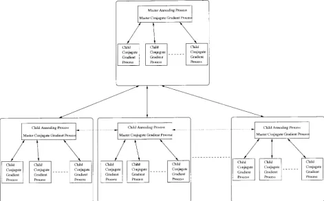
A two-level parallelism approach for computation of algorithm at the finer level is transparent to the parallel stochastic hill-climbing algorithms at the coarser level. the maximum-likelihood estimator:To ensure a scalable
implementation, two levels of parallelism were incorpo- In other words, the communication and control scheme for the parallel stochastic hill-climbing algorithms is rated in the computation of the maximum-likelihood
estimator. The finer or lower level of parallelism per- independent of that of the parallel conjugate gradient descent algorithm. This enhances the modularity and tains to the computation ofYˆfor a given probe ordering
⌸using the parallel conjugate gradient descent algo- flexibility of the system. For example, one could use the serial or parallel version of the conjugate gradient rithm for continuous optimization as discussed
Figure 8.—Master pro-cess for the parallel conju-gate gradient descent algo-rithm.
or parallel algorithm for continuous deterministic opti- tic hill-climbing process, a new set of child conjugate gradient descent processes is spawned on the available mization at the finer level without having to make any
changes to the parallel stochastic hill-climbing algo- processors, whereas the master conjugate gradient de-scent process runs on the same processor as the stochas-rithms at the coarser level.
The interaction between the master and child stochas- tic hill-climbing process (master or child). The master and child conjugate gradient descent processes cooper-tic hill-climbing (i.e., annealing) processes (NILM/
PILM PSA/PMCA) is shown with the double-headed ate to evaluate and minimize the value of the objective function for a specific probe ordering ⌸. Once the arrows between the larger components in Figure 10. A
parallel conjugate gradient descent algorithm is embed- objective function is evaluated, the child conjugate gra-dient descent processes terminate, and the correspond-ded within each of the stochastic hill-climbing processes.
stochas-Figure9.—Child process for the parallel conjugate gradient descent algorithm.
dient descent processes is depicted by the double- stochastic hill-climbing processes, and the second level is the group of processors that run the child conjugate headed arrows within each of the major components in
Figure 10. gradient descent processes. The processors that run the child conjugate gradient descent processes are con-The two-level parallelism approach can be seen to
induce a logical tree-shaped interconnection network nected to the processor running the parent stochastic hill-climbing process but are independent of the proces-on the processors in the PVM system. The first level is
Figure10.—The two-level parallel computation of the maximum-likelihood estimator.
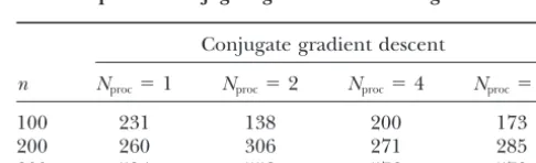
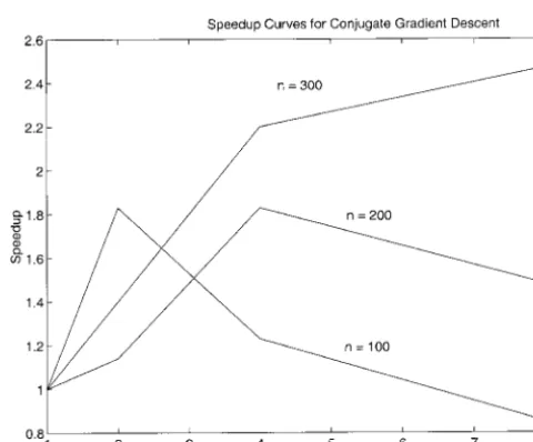
EXPERIMENTAL RESULTS when the maximum number of iterations was reached or when the number of successful perturbations equaled Experimental results on simulated data:The parallel
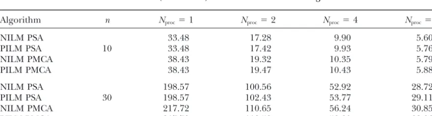
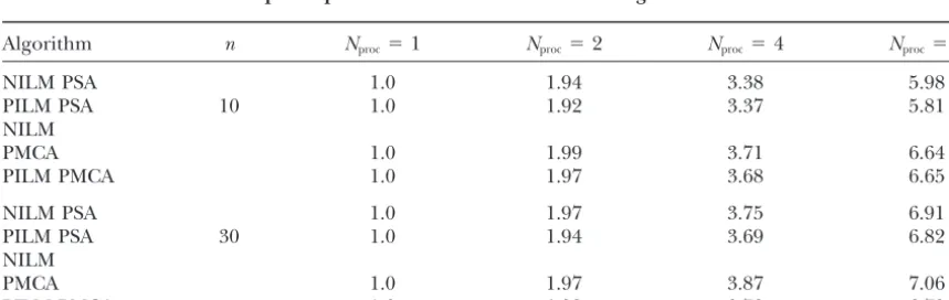
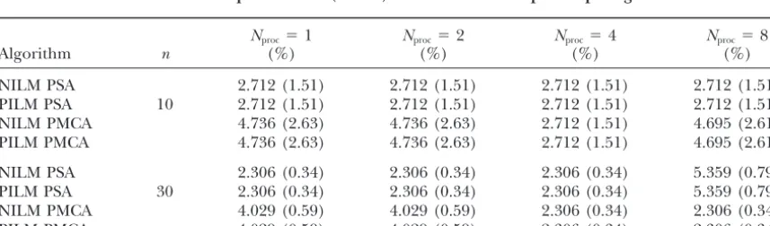
10 ·n(i.e., 10% of the maximum number of iterations), algorithms were implemented on a dedicated PVM
clus-whichever was encountered first. The temperature or ter of 200-MHz PentiumPro processors running
Solaris-demon energy values were systematically reduced at the x86 and tested with artificially generated clone-probe
end of each annealing step, using a geometric annealing hybridization data (Shete1998). Two sets of artificial
schedule with the annealing factor␣ ⫽0.95. The algo-data were used with the specifications outlined in Table
rithm was terminated (and deemed to have reached a 2. The artificial data were generated using a program
global optimum) when the number of successful pertur-described inShete(1998), which generates clonal data
bations in any annealing step equaled 0. of a given length with the left endpoints of the clones
In the case of the parallel stochastic hill-climbing algo-and probes uniformly distributed along the length of
rithms (NILM PSA, PILM PSA, NILM MCA, and PILM an artificial chromosome.
MCA) the product ofNprocand the maximum number The serial stochastic hill-climbing algorithms (SA and
of iterations D performed by a processor in a single MCA) were implemented with the following
parame-annealing step was kept constant, i.e., D⫽ (100 · n)/ ters: the initial value for the temperature or demon
Nproc. This ensured that the overall workload remained energy was chosen to be 0.5, and the maximum number
constant as the number of processors was varied, thus of iterations D for each annealing step was chosen to
enabling one to examine the scalability of the speed-be 100 ·n.The current annealing step was terminated
up and efficiency of the algorithms for a given problem size with increasing number of processors. The other
TABLE 2 parameters for the parallel stochastic hill-climbing algo-rithms were identical to those of their serial
counter-Specifications of the artificially generated
parts. In the NILM PSA and NILM PMCA algorithms,
clone-probe hybridization data
each process was independently terminated when the number of successful perturbations in any annealing
step for that process equaled 0. In the PILM PSA and
Data set n k N M (%) (%)
PILM PMCA algorithms, each process was terminated
Data set 1 10 100 180 15 2 2
when the number of successful perturbations in an
an-Data set 2 30 400 680 20 2 2