Copyright2000 by the Genetics Society of America
A Mixed-Model Approach to Mapping Quantitative Trait Loci
in Barley on the Basis of Multiple Environment Data
Hans-Peter Piepho
Institut fu¨r Nutzpflanzenkunde, FB 11, Universita¨t Kassel, 37213 Witzenhausen, Germany Manuscript received March 22, 2000
Accepted for publication July 25, 2000
ABSTRACT
In this article, I propose a mixed-model method to detect QTL with significant mean effect across environments and to characterize the stability of effects across multiple environments. I demonstrate the method using the barley dataset by the North American Barley Genome Mapping Project. The analysis raises the need for mixed modeling in two different ways. First, it is reasonable to regard environments as a random sample from a population of target environments. Thus, environmental main effects and QTL-by-environment interaction effects are regarded as random. Second, I expect a genetic correlation among pairs of environments caused by undetected QTL. I show how random QTL-by-environment effects as well as genetic correlations are straightforwardly handled in a mixed-model framework. The main advantage of this method is the ability to assess the stability of QTL effects. Moreover, the method allows valid statistical inferences regarding average QTL effects.
T
HERE are several different strategies to map quan- ian methods using cofactors (Sillanpa¨a¨ and Arjas 1998).titative trait loci (QTL; Kearsey and Farquhar
1998),e.g., single-marker locus analysis (Liu1998); sim- In this article, I analyze the barley dataset by the North American Barley Genome Mapping Project (Hanand ple interval mapping (IM;LanderandBotstein1989);
composite interval mapping (CIM;Zeng 1993, 1994), Ullrich 1993). This dataset comprises 16 trials per-formed in different environments. The aim of the analy-also called multiple QTL mapping (MQM;Jansenand
Stam 1994); simplified CIM (Tinker and Mather sis is to detect QTL with significant mean effect across environments and to characterize the stability of effects 1995); marker regression (KearseyandHyne1994;Wu
andLi1994); Bayesian methods (Sillanpa¨a¨andArjas across multiple environments. A need for mixed model-ing arises in two ways. First, for an assessment of mean 1998); and multiple interval mapping (MIM;Kaoet al.
1999;Zenget al.1999). The latter methods have been effects and of stability, it is necessary to regard environ-ments as a random factor. Second, I expect a genetic shown to yield better power of QTL detection than IM
and single-marker locus analysis (Liu1998;Lynchand correlation among pairs of environments caused by un-detected QTL (Korol et al. 1998). Random QTL-by-Walsh1998). In this article the main focus is on CIM
for its simplicity and its importance in practice. environment effects as well as genetic correlations are straightforwardly handled in a mixed-model framework. Within a frequentist framework, two different
model-fitting approaches can be distinguished among pro- The main advantage of my method is the ability to assess the stability of QTL effects. Moreover, the method allows cedures for QTL mapping by CIM: those based on
maximum-likelihood (ML) estimation (Lander and valid statistical inferences regarding average QTL ef-fects.
Botstein 1989;Zeng1994) and those using multiple linear regression (HaleyandKnott1992; Martinez andCurnow1992, 1994). The latter approach usually
MATERIALS AND METHODS gives results very similar to the former, though it must
be seen as an approximate method. The main advantage The data:I use the six-row Steptoe/Morex mapping popula-of the multiple regression approach is its computational tion by the North American Barley Genome Mapping Project simplicity (MartinezandCurnow1994). The compu- (Hanand Ullrich1993). The data comprise 150 doubled haploid (DH) lines, 223 markers, and 16 environments in the tational tradeoff may become quite considerable in
com-United States and Canada in 1991 and 1992. The same 150 plex situations,i.e., when the model is extended to cover
genotypes were tested in all environments. The data are par-several random effects, as in this article. I therefore
tially replicated with two replications. I use genotype-by-envi-prefer the regression approach to ML and also to Bayes- ronment means for different analyses.
The model for a single environment: The model will be
adjusted to DH and backcross progeny data, but it is readily extended for F2and other populations. Assume that the F1
Address for correspondence:Institut fu¨ r Nutzpflanzenkunde,
Universi-cross isM1QM2/m1qm2with respect to the two flanking markers
ta¨t Kassel, Steinstrasse 19, 37213 Witzenhausen, Germany.
E-mail: [email protected] bordering the interval of interest (M1andM2) and the QTL
where  ⫽ (, ␣, ␥⬘)⬘ with ␥ ⫽ (␥1, ␥2, . . . )⬘, xⴕi ⫽
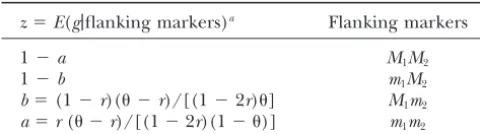
TABLE 1
(1,zi,cⴕi), and ciⴕ⫽(c1i,c2i, . . . ). The parameter vector is
Expectation of gconditional on flanking markers for a DH easily extended to include multiple QTL and effects for
epista-population (MartinezandCurnow1992) sis (Moreno-Gonzalez1992), but this is not elaborated here.
Model for data from multiple environments: The basic
model (1) may be taken as a building block for more refined z⫽E(g|flanking markers)a Flanking markers
modeling to account for the design. Here, I am particularly
1⫺a M1M2 interested in modeling data from multiple-environment trials
1⫺b m1M2 (METs). Specifically, I contend that a realistic model for
geno-b⫽(1⫺r)( ⫺r)/[(1⫺2r)] M1m2 type-by-environment effects is needed to make unbiased infer-a⫽r( ⫺r)/[(1⫺2r)(1⫺ )] m1m2 ences regarding QTL effects and positions. Moreover, the problem of genetic correlation among environments needs ar, recombination frequency between left flanking marker
to be taken into account in case the same set of genotypes is and QTL;, recombination frequency between both flanking tested in the different environments (Korolet al.1998). Let
markers. y
ijbe the observation of theith genotype (i⫽1, . . . ,N) in thejth environment (j⫽1, . . . ,M). The proposed model is
(Q). Define a random variablegifrom theith genotype taking
yij⫽ ⫹ ␣zi⫹ ␥1c1i⫹ ␥2c2i⫹. . .⫹ei valuegi⫽1 if the F1gamete carries theQallele andgi⫽0 if
the F1gamete carries theqallele. In the regression approach ⫹u
j⫹ajzi⫹g1jc1i⫹g2jc2i⫹. . .⫹dij. (3) to QTL mapping (Haley andKnott 1992; Martinez and
Curnow1992), the phenotype is regressed on the expected This model is derived by regarding all regression parameters value ofgi, given the flanking markers. Table 1 gives explicit in (1) as means across environments and allowing an environ-expressions forzi⫽E(gi|flanking markers) assuming no inter- ment-specific deviation. Thus, the environmental main effect ference (MartinezandCurnow1992). Missing marker data u
jcorresponds to,ajis a deviation of the QTL effect from can be handled using the method ofMartinezandCurnow the average␣in thejth environment,g
kj(k⫽1, 2, . . . ) is a (1994). In the case of backcross progeny, the genetic effect deviation from the average cofactor regression coefficient␥
k forziconstitutes a mixture of additive and dominance effects, (k⫽1, 2, . . . ) in thejth environment, andd
ijis a random whereas for doubled haploids, the genetic effects are confined deviation for theith genotype in thejth environment from to additive effects. For CIM using DH data, the following basic
the “average” residual effectei.Note that as opposed to (1), regression model can be used (Lynch andWalsh 1998, p.
eiin (3) is a residual genetic effect for theith genotype, which 465),
is free of experimental error. The experimental error is now captured bydij, which models both error and residual geno-yi⫽ ⫹ ␣zi⫹ ␥1c1i⫹ ␥2c2i⫹. . .⫹ei, (1)
type-by-environment interaction. An alternative way of deriv-whereyiis a phenotypic observation for theith genotype (i⫽ ing (3) is to allow a separate model of the form (1) for each 1, . . . ,N);is an intercept term;␣is the effect of the putative environment, to then combine all models into a single model, QTL; c1i, c2i, . . . are cofactors corresponding to markers on and finally to partition model parameters into average effects the map, which control for other QTL; ␥1, ␥2 . . . are the across environments and environment-specific deviations. associated regression coefficients; andeiis a residual account- All environment-specific deviations (uj,aj,gkj, anddij) and ing for both environmental variation and unexplained genetic the residual genetic effecteiare regarded as random normal variation. The residual genetic variation modeled byeiis re- deviates. To fully state the model, I need to specify the vari-garded as random. If the unexplained residual genetic varia- ances and covariances of all random terms. The variance-tion captured by ei is made up of a sum of small genetic covariance structure should allow sufficient generality to realis-contributions, the normality assumption foreimay be a suitable tically model real data. Before stating the full second moment approximation. Note, however, thateiwill also contain a com- assumptions, model (3) is modified to allow more generality. ponent due to the different genetic effects at the putative Model (3) contains a residual genetic effecte
iand a residual QTL, so a more realistic model is a mixture of normal distribu- d
ij.This model corresponds to the usual factorial partition-tions, with the number of components depending on the ing of main effects and interaction for genotype-by-environ-number of genotypes at the putative QTL. The normality ment data in plant breeding and quantitative genetics (Lynch assumption foreiis a matter of convenience, allowing model andWalsh1998). To highlight the fact thatd
ijcontains both fitting by ordinary least squares in the familiar regression error and genotype-by-environment interaction, I may write framework, rather than by ML. Several authors have pointed d
ij⫽fij⫹hij, wherefijis the interaction andhijis error. The out that using least squares in place of ML tends to cause customary assumption in mixed-model analyses, henceforth only a marginal loss of information (HaleyandKnott1992; denoted as compound symmetry assumption, is that
ei,fij, and MartinezandCurnow1992). Also, ML estimation has large
hij are identically distributed with zero mean and constant sample optimality properties only when the model is correctly
variances,2
e,2f, and2h, respectively. This assumption is quite specified. In most applications, the true underlying genetic
restrictive because it implies constancy of genetic correlation model will be complex and any fitted model can at best be
among pairs of environments as well as constancy across envi-regarded as an attempt to approximate the true model as
ronments of genetic variances within environments. For this closely as possible (BurnhamandAnderson1998). If there
reason, I replace the termei ⫹dijby a term eijand initially are a number of QTL not accounted for by the fixed part of
assume that the random vectorei⫽(e1i, . . . ,eiM)⬘has unstruc-the model and errors are normal, unstruc-the residual will be a mixture
tured variance-covariance matrix var(ei)⫽R, whereRis sym-of an unspecified number sym-of component normals.
Approxi-metric and positive definite. I then explore various structured mating this mixture by a normal distribution should be
ade-models for R, which have fewer parameters than in the un-quate in most circumstances. Model (1) may be expressed in
structured case. The compound symmetry assumption is vector notation as
IM is the M-dimensional identity matrix, and 2⫽ 2f ⫹ 2h. diagonal elements may be either homogeneous (R⫽IM2) or heterogeneous (R⫽D).
The modified scalar model reads
QTL-by-environment effects and environmental main effect:In my yij⫽ ⫹ ␣zi⫹ ␥1c1i⫹ ␥2c2i⫹. . . analysis inferences are to be drawn with respect to a target population of environments. I regard the testing
environ-⫹uj⫹ajzi⫹g1jc1i⫹g2jc2i⫹. . .⫹eij. (4)
ments as a random sample from the target. The purpose of a mixed-model analysis is to reveal mean QTL effects across In vector notation this can be written as
environments. Here, random QTL-by-environment interac-tion essentially plays the role of an error term. Moreover, the yij⫽ⴕxi⫹b⬘jxi⫹eij, (5)
stability of QTL effects across environments is an important where is as defined in (1) and bj⫽(uj,aj,g⬘j)⬘withgj⫽ aspect. The larger the variance of QTL-by-environment effects (g1j, g2j, . . . )⬘. The main interest of our analysis is in the the lower the stability. Finally, I can make environment-specific average QTL effects in, while the random vectorbjbasically inferences, employing best linear unbiased predictions plays the role of an error term. To cater for generality, correla- (BLUPs) of QTL-by-environment effects.
tion among elements inbjis allowed. Details are discussed in It is necessary to allow for correlation among the effects in the next paragraphs. A desirable feature of the model is this: bj. For example, a perfect correlation must be assumed for instead of dropping certain genetic effects completely, I can regression coefficients pertaining to adjacent markers, since choose whether to move them to and bj, or toeij. I now both are linear in the additive genetic effect of the flanked discuss suitable variance-covariance structures foreijandbj. QTL (Whittakeret al.1996). Also, variances of two compo-Genotype-by-environment effects:I regard the genetic compo- nents in (bj) corresponding to a pair of markers will have to nents ineijas random. When testing the same set of genotypes be heterogeneous, considering the explicit expressions given in the various environments, as has been assumed so far, inWhittakeret al.(1996, p. 25, right, bottom). Moreover, genetic correlation among observations on the same genotype different QTL may be responding similarly to differential envi-made in different environments needs to be allowed for. Many ronments, giving rise to positive correlation among regression articles on the mapping of QTL based on multienvironment coefficients corresponding to markers adjacent to different data corresponding to this design (Jansenet al.1995;Beavis QTL. For these reasons I make the general assumption that andKeim1996;Romagosaet al.1996;Sari-Gorlaet al.1997;
var(bj)⫽G, (6)
Korolet al.1998) have employed a multiple regression model
with independent errors. This model implicitly assumes ab- whereG is symmetrical and positive definite, but otherwise sence of genetic correlation, which is an unrealistic assump- unstructured. Note that this assumption also ensures scale tion. It is to be expected that in the presence of positive genetic invariance,i.e., invariance to the particular coding for markers correlation, the information on QTL position provided by (0/1, 1/2,⫺1/1). Again, explicit modeling of the variance-data from a sample of environments is smaller than when covariance structure is worthwhile to keep the number of genetic correlation is absent. This is best explained by a simple parameters low, although many parsimonious structures suffer example (not specifically designed for QTL analysis). Con- from lack of scale invariance. I can consider the same struc-sider two observationsy1and y2. The mean (y1⫹ y2)/2 has tures as forR. It should be stressed thatGdoes not contain variance (2
1⫹ 22⫹212)/4, where21and22are the vari- genetic effects, but merely QTL-by-environmental effects and ances ofy1andy2, respectively, andis the correlation. Clearly, an environmental main effect.
the variance of the mean is an increasing function of the The effect of the putative QTL in thejth environment is correlation. Similarly, in QTL mapping, accuracy of parame- given by (␣ ⫹aj). The diagonal element inGcorresponding ter estimates is expected to decrease with genetic correlation. toajcan therefore be interpreted as a measure of stability of Ignoring genetic correlation can therefore lead to overopti- the effect of the putative QTL. The larger the variance ofaj, the mistic inferences,i.e., to spurious detections and to inappro- more variable/less stable are the environment-specific QTL priate standard errors for parameter estimates. For this reason, effects (␣ ⫹aj). The breeder will seek a large absolute value I principally allow correlations among elements inei.A varie- for ␣ and a small variance for aj, i.e., a high stability. This ty of models forR ⫽ var(ei) can be considered. The most interpretation of a variance component as a measure of QTL complex choice leavesRunstructured, and the simplest model effect stability is akin to approaches for assessing yield stability isR⫽IM2. While the unstructured model is often the most in MET data (Linet al.1986;BeckerandLe´on1988;Piepho realistic one, it may entail an unnecessarily large number of 1998b).
parameters, when the number of environments (M) is large. It is convenient to write the full model foryijin matrix form Overparameterization may be avoided by imposing a certain as
variance-covariance structure. I consider models commonly
y⫽(1M丢X)⫹(IM丢X)b⫹e, (7) used for the analysis of genotype-by-environment data,i.e.,
compound symmetry (R⫽JM2e⫹IM2), heteroscedastic (R⫽ where y ⫽(y
11, . . . ,yN1, y12, . . . ,yNM)⬘, 1Mis a vector ofM DandR⫽JM2g⫹D, whereDis a diagonal matrix;Shukla ones,X⫽(x1, . . . ,x
N)⬘,⫽(,␣,␥⬘)⬘,IMis theM-dimensional 1972), and various factor-analytic models, which are character- identity matrix, b⫽(b⬘1, . . . ,b⬘
M)⬘, and e ⫽ (e11, . . . , eN1, ized by a componentⴕ, where⫽(1, . . . ,M)⬘is a vector e
12, . . . ,eNM)⬘. Apart from the residual variance, this model is of factor loadings associated with the individual environments similar to the random effects model for longitudinal data (Piepho1998a). The simplest factor-analytic variance-covari- (Lairdand Ware1982). The first two moments under this ance structure is given byR⫽ⴕ⫹IM2, corresponding to model are
the modeleij⫽ jui⫹wij, whereuiis a standard normal score
for theith genotype and wij is normal with zero mean and E(y)⫽(1M丢X) (8)
variance2. Environments with a large absolute value for the
and factor loadingjwill have residualseijmore widely spread out
than environments with smallj. I note in passing that model var(y)⫽I
M丢XGXⴕ⫹R丢IN. (9) (3) is also applicable if a different set of genotypes is tested
it is tempting to compute genotype means across environ- TABLE 2
ments and subject these to standard CIM. Such an analysis
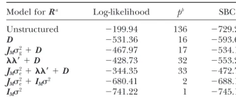
Fitting information for different models forR
assumes that means of different genotypes,y⫽M⫺1(1ⴕ M丢IN)y, are stochastically independent and have homoscedastic errors
Model forRa Log-likelihood pb SBC
(Mis the number of environments). This assumption is prob-lematic with model (5), under which I have for the means
Unstructured ⫺199.94 136 ⫺729.20
E(y)⫽X (10) D ⫺531.36 16 ⫺593.63
JM2g⫹D ⫺467.97 17 ⫺534.13
and ⴕ⫹
D ⫺428.73 32 ⫺553.26
JM2e⫹ⴕ⫹D ⫺344.35 33 ⫺472.77
var(y)⫽M⫺1XGXⴕ⫹I
N2R, (11)
JM2e⫹IM2 ⫺680.41 2 ⫺688.19
where 2
R⫽M⫺21⬘MR1M. The important point to note here is I
M2 ⫺741.22 1 ⫺745.11
that all elements inyare correlated among one another due to the termM⫺1XGXⴕon the right-hand side of (11). Thus,
Environment main effects and QTL-by-environment inter-the means y violate the assumptions underlying a standard action effects are regarded as fixed. Models fitted by REML. QTL analysis. An appropriate means analysis could be based aD, a diagonal matrix; J
M, a square matrix of ones every-on generalized least squares using (11), but this is not recom- where; , column vector of M factor loadings; IM, the mended for two reasons. First, using (11) requires an estimate M-dimensional identity matrix.
of G, which necessitates an analysis of replicate data, thus bp, number of parameters for the variance-covariance ma-annihilating the computational advantages of the means analy- trixR.
sis. Second, and more importantly, the means themselves are unweighted and thus ignore the genetic correlation structure. Therefore the means analysis is not optimal.
proach is of anad hocnature, considering the fact that strictly
Model selection:In what follows I assume random
environ-speaking the means violate the independence assumption. As ments and consider CIM for mean QTL effects across
environ-more efficient software becomes available, applying MPS to the ments. Model selection is necessary regarding three aspects:
replicate data using a mixed-model framework is preferable. (1) the markers to be used as cofactors, (2) the
variance-Genotype-by-environment interaction (R):I initially assume the covariance structure forR, and (3) the model for
QTL-by-most general model for QTL-by-environment interaction on environment interaction,i.e., forG.These selection problems
the basis of the genetic model corresponding to the selected are briefly discussed. Unfortunately, the three problems
can-cofactors (Wolfinger 1993). At this stage, the model does not be tackled in an entirely independent manner. For
exam-not yet contain the covariatezifor the pair of markers flanking ple, in a joint analysis of the data, the chosen
variance-covari-the putative QTL. Interactions are regarded as fixed, although ance model will have an effect on the selected set of markers
at later steps of the analysis I take QTL-by-environment interac-and vice versa. From a theoretical point of view it seems
desir-tion as random. No specific model is assumed for the interac-able to handle these three model components simultaneously.
tions. The model I select for R is used subsequently when Due to the large number of candidate models (i.e.,
combina-modeling QTL-by-environment interaction and when scan-tions of choices for 1–3), however, this simultaneous approach
ning the genome for putative QTL. is not usually feasible in practice. Thus, some form of
sequen-QTL-by-environment interaction and environmental main effect tial approach is preferable. While this may entail the risk
(G):I now take QTL-by-environment interactions and the envi-of missing some good-fitting models, it has the important
ronmental main effect as random. Thus, I have the task of advantage of reducing the total number of models to be
con-selecting an appropriate variance-covariance structure forG. sidered. I suggest to first select the markers, then the
variance-The need for invariance under recoding of the markers dic-covariance structure forR, and finally the model for
QTL-by-tates the unstructured model forG, while the parsimony prin-environment interaction (G). At each step, I use the Schwarz
ciple suggests that simpler approximating structures may be Bayesian Criterion (SBC) to choose among options
(Wol-worth considering. I propose to generally fit an unstructured finger 1993; McQuarrieand Tsai1998). The criterion is
model, except when the dimension ofGis large and an un-given by SBC⫽logL⫺1⁄
2plog(n), whereLis the maximized structured model is difficult to fit. likelihood,pis the number of parameters, andnis the number
Scanning the genome:The same model as selected for both
of observations. Models with large values for SBC are
pre-R and G in the previous steps is used when scanning the ferred.
genome for QTL. Of course,RandGare reestimated at each Cofactor selection:I select cofactors by multiple linear
regres-putative QTL position. Note thatGis extended at the scanning sion of meansyon marker types using the marker pair
selec-stage by the covariatezifor the two flanking markers. Assuming tion (MPS) approach by H.-P. Piepho and H. G. Gauch
the same structure as selected for the case wherexicontains (unpublished results). This procedure has three distinctive
only the cofactors may not be optimal. It would not be practica-features: (i) markers are selected in adjacent pairs to increase
ble, however, to select a different model at each step during the chance of selecting flanking markers while reducing the
the genome scan. Also, the type of model finally chosen for risk of selecting markers not linked to QTL; (ii) an exhaustive
RandGnot only depends on model fit but also on ease of search per chromosome is used in place of simple forward
estimation. Some structures forRand Gmay be well fitting selection, which reduces the risk of missing the best fitting
but difficult to estimate (convergence problems, difficulty in model; (iii) a model selection criterion such as SBC is
em-choosing good starting values, etc.), thus making them infeasi-ployed to select the final model among a sequence of models.
ble for automated QTL scans, where the same model has to Among a selected pair, I use the marker that fits best as a
be estimated a large number of times. cofactor for CIM. The procedure was developed for models
with a single error term. Extension to the mixed model (4) for the replicate data is straightforward in principle but not
generally feasible at present, mainly because of the prohibitive EXAMPLE workload of having to fit a multitude of complex models by
I used the barley data to exemplify the proposed ML or restricted maximum likelihood (REML). This is the
Be-TABLE 4 TABLE 3
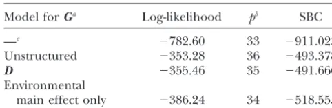
Fitting information for different models forG Parameter estimates for fixed effects and standard errors
(SE) based on analysis of means and a mixed-model
analysis withR⫽JM2e⫹ⴕ⫹Dand unstructured
Model forGa Log-likelihood pb SBC
G(includes a cofactor for M82, but
—c ⫺782.60 33 ⫺911.023
no effect for putative QTL)
Unstructured ⫺353.28 36 ⫺493.378
D ⫺355.46 35 ⫺491.666
Analysis of means Mixed model Environmental
main effect only ⫺386.24 34 ⫺518.555 Parameter Estimate SE Estimate SE
Mixed-model analysis withR⫽JM2e⫹ⴕ⫹D. Model fit- Intercept 5.56 0.040 5.55 0.368
ted by REML. M82 ⫺0.50 0.055 ⫺0.49 0.112
aD, a diagonal matrix.
bp, number of parameters for the whole variance-covariance Model fitted by REML. structure,i.e., forRandG. The model forRhas 33 parameters
in all cases.
cThis model has no random effects corresponding toG.
covariatezifor the putative QTL. This again raises the question of how to modelG. A priori, the unstructured model seems most appropriate, especially since there is tween these two, M82 had a better fit than M81 if fitted only one cofactor so that parsimony is not a pressing alone. Subsequently, the cofactor M82 and the interac- issue. Thus, I used the unstructured model. The window tions with environments were included in the fixed part size was 10 cM;i.e., for putative QTL within 10 cM of a of the model and various structures were fitted toRby cofactor, the cofactor was dropped from the model. The the REML method. At this stage,xidid not yet contain step size of the chromosome scan was 1 cM. During the a covariate zi for the putative QTL. All mixed-model chromosome scan, parameter estimates for G and R analyses were done using ASREML (Gilmour et al. from the present putative QTL position were used as 1999). The same genotypes have been tested in all envi- starting values at the next position. This resulted in ronments, so genetic correlation needs to be modeled convergence of the REML algorithm within a few itera-inR. Since there areM⫽16 environments and hence tions (typically 5–10). [One referee noted that this
Ris a M ⫻ M matrix, there are M(M ⫹ 1)/2 ⫽ 136 choice of starting values may cause convergence to a parameters for the unstructured model. The results for local, but not the global maximum of the (restricted) different models are shown in Table 2. On the basis of log-likelihood. In my experience the likelihood of this SBC the factor-analytic modelR⫽ JM2e ⫹ ⴕ⫹Dwas problem is small with a short step size. In the present
selected. example the problem was not observed. The same
ref-The Wald F-statistic for cofactor(M82)-by-environ- eree indicated that using fixed starting values gives more ment interaction inbwas 10.84, which is significant at stable results.] At each position, I computed a Wald
Figure 1.—Fprofile for composite interval mapping based on mixed model for genotype-by-environment data (left, critical threshold atF⫽ 12.83) and on simple regression model for geno-type means across environments (right, critical threshold atF⫽13.01). Chromosomes 1–7.
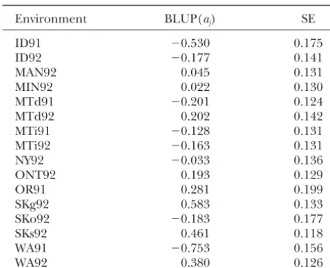
mixed-model analysis. Since the estimated QTL position 0.10, where⌽is the cumulative density function of the is within 10 cM of the cofactor M82, this cofactor was standard normal distribution. Table 5 gives BLUPs ofaj. dropped for the analysis at this position. The estimate For 1 out of the 16 environments (SKg92), the resulting forGwas estimate of␣ ⫹ajhas a positive sign. This finding is in good agreement with the estimated probability of 10%. Thus, despite the relatively large average QTL effect,
Gˆ ⫽
冢
2.14 ⫺0.296⫺0.296 0.137
冣
. some surprises are possible in specific environments.Thus, the variance of environmental main effects was 2.14, which is notably larger than the variance of the
DISCUSSION QTL effects across environments (0.137). The variance
A common feature of QTL analyses is that QTL effects of QTL effects corresponds to a standard deviation of
depend on environment. Many researchers have dealt 0.370, which is fairly large relative to the average QTL
with this problem by analyzing each environment sepa-effect␣. This shows that the detected QTL is not very
rately. This approach is quite useful, if one is interested stable across environments. For example, assuming
nor-in the particular test environments. As ponor-inted out by mality, the probability that the QTL effect in a randomly
TinkerandMather(1995), “separate analysis by envi-chosen environment (given by␣ ⫹aj) has positive sign
QTL-TABLE 5 ences, the main one being thatWanget al.(1999) do not allow for genetic correlation. They exploit map
in-BLUPs of QTL-by-environment effectsajat position 58.9 cM
formation to model the equivalent of my G. This
ap-on chromosome 3 in mixed-model analysis with
proach requires a specific genetic model, including
epis-R⫽JM2e⫹ⴕ⫹Dand unstructuredG
tasis and specification of multiple QTL. It assumes that
Environment BLUP(aj) SE all genetic effects are modeled byGand that all
correla-tion among effects is solely due to the map. It is to be
ID91 ⫺0.530 0.175
expected that the approach is susceptible to
misspecifi-ID92 ⫺0.177 0.141
cation of the model. By contrast the model used in this
MAN92 0.045 0.131
article allows unexplained genetic effects and genetic
MIN92 0.022 0.130
MTd91 ⫺0.201 0.124 correlation to be subsumed in the residualeij.As a result
MTd92 0.202 0.142 there is no need to assume a specific overall model.
MTi91 ⫺0.128 0.131 Moreover, using a general model forGallows for
covari-MTi92 ⫺0.163 0.131 ance among QTL that is due to correlated response to
NY92 ⫺0.033 0.136
differential environmental condition. Such correlation
ONT92 0.193 0.129
can arise even for QTL on different chromosomes,
OR91 0.281 0.199
which would be regarded as independent under the
SKg92 0.583 0.133
SKo92 ⫺0.183 0.177 model used byWanget al.(1999). My model could be
SKs92 0.461 0.118 easily extended to exploit the map in modeling the
WA91 ⫺0.753 0.156 correlation among cofactors and the putative QTL in
WA92 0.380 0.126
G, but I prefer to work with a general model forGboth for ease of computation and to reduce the danger of Model fitted by REML.
model misspecification. Also, if the approach is ex-tended to multiple QTL and epistatic effects, it is still preferable to work with generalGfor the same reasons. by-environment interaction and avoids complications
due to environmental heterogeneity. However, the re- When the dimension ofGbecomes large, it is reasonable to consider more parsimonious models such as those sults of separate analyses are difficult to interpret, and
they do not take advantage of the built-in replication used forR.
In this article I have demonstrated how to use mixed provided by multiple environments.” Quite frequently,
test environments are just a sample from a target popula- models for assessing mean and stability of QTL effects based on genotype-by-environment means from MET tion, and the breeder is interested in making broad
inferences not restricted to the particular test environ- data. My mixed-model framework is easily extended to other settings,e.g., when spatial heterogeneity needs to ments (Melchinger et al. 1998). This objective calls
for a mixed-model analysis with random environments be modeled at the plot level (nearest neighbor analyses; Moreauet al.1999) and when the experimental designs (BeavisandKeim1996). The present article has shown
how to implement such an analysis for CIM. The ap- give rise to random effects (incomplete blocks, etc.; HaleyandKnott1992). Error variance heterogeneity proach is easily extended to cover multiple-QTL and
epistatic effects by appropriate modifications ofand among different environments in MET can be ac-counted for by weighting (Culliset al.1996), though
bj(Moreno-Gonzalez1992;Wanget al.1999). This is
useful as an additional analysis step, when several QTL in my experience weighting has little effect on final parameter estimates and standard errors.
have been detected by CIM.
A simple alternative to a mixed-model analysis of MET My analysis has assumed random environments. In a model with fixed environments, the focus is on studying QTL data is to proceed in two steps as follows: first, the
quantitative trait is analyzed by ANOVA techniques to QTL-by-environment interactions. It has been stressed byKorolet al. (1998) that the number of interaction obtain (adjusted) genotype means across environments.
Second, the means together with the marker data are parameters in models such as (4) increases linearly with the number of environments. These authors used the submitted to a routine for QTL analysis. My theoretical
considerations and analysis of a real dataset led me to regression approach ofEberhartandRussell(1966) to model interactions with fewer parameters. The re-conclude that such analyses may lead to inappropriate
inferences, mainly because standard error estimates are gression approach by Eberhart and Russell(1966) was originally proposed for the analysis of genotype-by-inappropriate. A mixed-model framework allows more
valid inferences to be obtained by incorporation of dif- environment interaction, but it can be applied in the same way to model QTL-by-environment interaction, as ferent random components of variance that
appropri-ately account for the environmental and genetic struc- demonstrated byKorolet al.(1998). In fact, there are a large number of different models for genotype-envi-ture of the data.
differ-Lander, E. S.,andD. Botstein,1989 Mapping Mendelian factors
which are potentially useful for modeling
QTL-by-envi-underlying quantitative traits using RFLP linkage maps. Genetics
ronment interaction. This potential seems to have gone 121:185–199.
largely unnoticed in QTL work. For example, extensions Lin, C. S., M. R. BinnsandL. P. Levkovitch,1986 Stability analysis: where do we stand? Crop Sci.26:894–900.
of the Eberhart-Russell regression such as the additive
Liu, B.-H.,1998 Statistical Genomics.CRC Press, Boca Raton, FL.
main effects multiplicative interaction model (Gauch Lynch, M.,andB. Walsh,1998 Genetics and Analysis of Quantitative 1988) typically explain a much larger fraction of the Traits.Sinauer, Sunderland, MA.
Martinez, O.,andR. N. Curnow,1992 Estimating the locations
total interaction and so promise improved performance
and the sizes of the effects of quantitative trait loci using flanking
(Romagosaet al.1996). These approaches can be incor- markers. Theor. Appl. Genet.85:480–488.
porated into my mixed model by takingbas fixed and Martinez, O., andR. N. Curnow, 1994 Missing markers when estimating quantitative trait loci using regression mapping.
He-imposing some structure such as in Eberhart-Russell
redity73:198–206.
regression. McQuarrie, A. D. R.,andC.-L. Tsai,1998 Regression and Time Series Model Selection.World Science Publishing Company, Singapore. Thanks are due to Hugh Gauch Jr. and Susan McCouch for inspiring
Melchinger, A. E., H. F. UtzandC. C. Scho¨ n,1998 Quantitative discussions. H.F. Utz (University of Hohenheim, Germany) is thanked
trait locus (QTL) mapping using different testers and indepen-for helpful comments on an earlier draft. Support of the Heisenberg
dent population samples in maize reveals low power of QTL Programm of the Deutsche Forschungsgemeinschaft is gratefully ac- detecting and large bias in estimates of QTL effects. Genetics knowledged. Part of the research for this article was conducted while 149:383–403.
the author was visiting the Department of Biometrics and the Depart- Moreau, L., H. Monod, A. Charcosset and A. Gallais, 1999 ment of Plant Breeding, College of Agriculture and Life Sciences, Marker-assisted selection with spatial analysis of unreplicated field
trials. Theor. Appl. Genet.98:234–242. Cornell University, Ithaca, NY.
Moreno-Gonzalez, J.,1992 Genetic models to estimate additive and non-additive effects of marker-associated QTL using multiple regression techniques. Theor. Appl. Genet.85:435–444.
Piepho, H. P.,1998a Empirical best linear unbiased prediction in
LITERATURE CITED cultivar trials using factor analytic variance-covariance structures.
Theor. Appl. Genet.97:195–201.
Beavis, W. D.,andP. Keim,1996 Identification of quantitative trait
Piepho, H. P.,1998b Methods for comparing the yield stability of loci that are affected by environment, pp. 123–149 in
Genotype-cropping systems—A review. J. Agron. Crop Sci.180:193–213.
by-Environment Interaction, edited byM. S. KangandH. G. Gauch
Romagosa, I., S. E. Ullrich, F. HanandP. M. Hayes,1996 Use
Jr.CRC Press, Boca Raton, FL.
of additive main effects and multiplicative interaction model in
Becker, H. C.,andJ. Le´on,1988 Stability analysis in plant breeding.
QTL mapping for adaption in barley. Theor. Appl. Genet.93:
Plant Breed.101:1–23.
30–37.
Burnham, K. P.,andD. R. Anderson,1998 Model Selection and
Infer-Sari-Gorla, M., T. Calinski, Z. KaczmarekandP. Krajewski,1997
ence.Springer, New York.
Detecting QTL⫻environment interaction in maize by a least
Cullis, B. R., F. M. Thomson, J. A. Fisher, A. R. GilmourandR.
squares interval mapping method. Heredity78:146–157.
Thompson,1996 The analysis of the NSW wheat variety data
Shukla, G. K.,1972 Some statistical aspects of partitioning geno-base. II. Variance component estimation. Theor. Appl. Genet.
type-environmental components of variability. Heredity29:237–
92:28–39.
245.
Davies, R. B.,1977 Hypothesis testing when a nuisance parameter
Sillanpa¨a¨, M. J.,andE. Arjas,1998 Bayesian mapping of multiple is present only under the alternative. Biometrika64:247–254.
quantitative trait loci from incomplete inbred line cross data.
Davies, R. B.,1987 Hypothesis testing when a nuisance parameter
Genetics148:1373–1388. is present only under the alternative. Biometrika74:33–43.
Tinker, N. A.,andD. E. Mather,1995 Methods for QTL analysis
Eberhart, S. A.,andW. A. Russell,1966 Stability parameters for
with progeny replicated in multiple environments. J. Quant. Trait comparing varieties. Crop Sci.6:36–40.
Loci1:http://probe.nalusda.gov:8000/otherdocs/jqtl/.
Gauch, H. G.,1988 Model selection and validation for yield trials
van Eeuwijk, F. A., J. B. DenisandM. S. Kang,1996 Incorporating with interaction. Biometrics44:705–715.
Gilmour, A. R., B. R. Cullis, S. J. WelhamandR. Thompson,1999 additional information on genotypes and environments in
mod-ASREML. User manual, ftp://ftp.res.bbsrc.ac.uk/pub/aar/. els for two-way genotype by environment tables, pp. 15–50 in
Haley, C. S.,andS. A. Knott,1992 A simple regression method Genotype-by-Environment Interaction, edited by M. S. Kang and for mapping quantitative trait loci in line crosses using flanking H. G. Gauch Jr.CRC Press, Boca Raton, FL.
markers. Heredity69:315–324. Wang, D. L., J. Zhu, Z. K. LiandA. H. Paterson,1999 Mapping
Han, F.,andS. E. Ullrich,1993 The North American Barley Ge- QTLs with epistatic effects and QTL⫻environment interaction nome Mapping Project: Mapping of quantitative trait loci associ- by mixed linear model approaches. Theor. Appl. Genet.99:1255–
ated with malting quality. Barley Genet. Newsl.23:84–97. 1264.
Jansen, R. C.,andP. Stam, 1994 High resolution of quantitative Whittaker, J. C., R. ThompsonandP. M. Visscher,1996 On the traits into multiple loci via interval mapping. Genetics136:1447– mapping of QTL by regression of phenotype on marker-type.
1455. Heredity77:23–32.
Jansen, R. C., J. W. van Ooijen, P. Stam, C. ListerandC. Dean, Wolfinger, R. D.,1993 Covariance structure selection in general
1995 Genotype-by-environment interaction in genetic mapping mixed models. Commun. Stat. A22:1079–1106.
of multiple quantitative trait loci. Theor. Appl. Genet.91:33–37. Wu, W.-R.,andW.-M. Li,1994 A new approach for mapping
quanti-Kao, C. H., Z-B. ZengandR. D. Teasdale,1999 Multiple interval tative trait loci using complete genetic marker linkage maps. mapping for quantitative trait loci. Genetics152:1203–1216. Theor. Appl. Genet.89:535–539.
Kearsey, M. J.,andA. G. L. Farquhar,1998 QTL analysis in plants; Zeng, Z-B.,1993 Theoretical basis of separation of multiple linked
where are we now? Heredity80:137–142. gene effects on mapping quantitative trait loci. Proc. Natl. Acad.
Kearsey M. J.,andV. Hyne,1994 QTL analysis: a simple ‘marker Sci. USA90:10972–10976.
regression’ approach. Theor. Appl. Genet.89:698–702. Zeng, Z-B.,1994 Precision mapping of quantitative trait loci.
Genet-Korol, A. B., Y. I. RoninandE. Nevo,1998 Approximate analysis ics136:1457–1466.
of QTL-environment interaction with no limits on the number Zeng, Z-B., C. H. KaoandC. J. Basten,1999 Estimating the genetic
of environments. Genetics148:2015–2028. architecture of quantitative traits. Genet. Res.74:279–289.
Laird, N. M., andJ. H. Ware, 1982 Random effects model for