ABSTRACT
SONG, TAI-JIN. Recurrent Freeway Bottlenecks Identification and Applications (under the direction of Dr. Billy M. Williams and Dr. Nagui M. Rouphail).
Traffic congestion and safety concerns are contributing to the many challenges facing
transportation agencies as population, motorization, and urban densities continue to rise.
Congestion is contributing to longer travel times, higher fuel consumption, and increased
emissions of air pollutants. Nearly 40% of roadway congestion in the United States stems
from recurrent bottlenecks, which can cost agencies both time and money if not properly
addressed.
Identification of recurrent bottlenecks is an effective way to hone in on appropriate
investment in current facilities to relieve congestion. Furthermore, it would enable the
ranking or prioritization of bottlenecks since bottleneck removal and its associated impact
alleviation are hampered by limited sources. It is imperative that transportation jurisdictions
identify the basis for ranking bottlenecks by exploring: how often they activate; how long it
takes the congestion to disappear; and how many miles of road are affected.
In this thesis, a data-driven approach for identifying recurrent bottlenecks
spatiotemporally is introduced, using probe vehicle speed reports. Historical spatiotemporal
characteristics of bottlenecks are investigated through a comprehensive analysis of statewide
interstates in North Carolina. Using the characteristics discovered, the recurrent bottleneck
locations with a historical time span of bottleneck activation are revealed and tested. The
There is also a chance that those same bottlenecks can be exacerbated when there
happen to be a crash within their area of impact. In other words, the crash results in
additional congestion on top of the recurrent congestion. Accordingly, this effect should be
identified and quantified separately when it comes to identifying and monitoring bottlenecks
and their associated impacts more accurately. Previous bottleneck studies have estimated
bottleneck impact with little attention to distinguishing the underlying source of congestion.
In addition, studies that have attempted to distinguish between recurrent and non-recurrent
congestion have focused on separating non-recurrent congestion from recurrent congestion
only for the purpose of estimating the intensity of congestion using parameters for the speed
distribution in a time of day in a segment or point. A data-driven methodology for
quantifying recurrent bottleneck impact is introduced, which quantifies recurrent and
collision-induced congestion impacts separately.
In order to quantify collision-induced congestion impacts, there needs to be a
thorough understanding of the conditions in which vehicles occur. An easily implementable
methodology that can classify all reported crashes in terms of the operational conditions
under which each crash occurred is presented. Unlike previous secondary crash classification
schemes, the proposed methodology requires neither a-priori identification of the
precipitating incident nor definition of the precipitating incident’s impact area.
Using 2014 statewide interstate data in North Carolina, a total of 95 bottleneck
segments were identified with the selected thresholds. Of these, an average two recurrent
bottlenecks occurred within a bottleneck impact area. Six bottlenecks were finally selected
by a systematic process and then used for identifying the statistical characteristics of
impacts. Recurrent bottleneck spatiotemporal impacts were calculated using the proposed
quantification scheme. The historical impacts varied from 1 to 3 mile-hours of impact per
activation except for the third study site which yielded 13 mile-hours per activation, and was
thus identified as the worst bottleneck among all the study sites. The impact factor can be
directly applied for ranking freeway bottlenecks and facilitates monthly and/or annual
analysis on a large scale network. In addition, it allows for identification of degraded or
improve recurrent bottleneck impact. The proposed approaches are robust and represent a
Recurrent Freeway Bottlenecks Identification and Applications
by Tai-Jin Song
A dissertation submitted to the Graduate Faculty of North Carolina State University
in partial fulfillment of the requirements for the degree of
Doctor of Philosophy
Civil Engineering
Raleigh, North Carolina
2016
APPROVED BY:
_______________________________ ______________________________
Billy M. Williams, Professor Nagui M. Rouphail, Professor
Co-Chair of Advisory Committee Co-Chair of Advisory Committee
________________________________ ________________________________
DEDICATION
To heavenly farther, my lovely wife, Aeri, and my two children, Ryan and Ian.
BIOGRAPHY
Tai-Jin Song is from Seoul, South Korea. He received his Bachelor and Master of
Transportation Systems Engineering from Hanyang University in 2008 and 2010,
respectively. Tai-Jin began working on his Doctor of Philosophy in Civil Engineering at
North Carolina State University in 2013 and anticipates completion in 2016. Before seeking a
PhD, Tai-Jin worked professionally for 4 years with the Korea Transport Institute. As a key
researcher, Tai-Jin conducted more than fifteen research and development government
ACKNOWLEDGMENTS
I would like to express a heartful gratitude to Dr. Billy M. Williams and Dr. Nagui M.
Rouphail. They gave me invaluable lessons in life and research as well as continuous support
for my research. Their guidance and passion made this work possible. I would also like to
thank Dr. George F. List and Dr. Justin Post for the advice and support provided as members
of my advisory committee.
A special thanks to Dr. Sankey Kim, Shannon Warchol, Kihyun Pyo, Juwoon Baek, J.
Lake Trask, Thomas Chase, and all other staff at the Institute for Transportation Research
and Education (ITRE) at North Carolina State University for helping and supporting my
TABLE OF CONTENTS
1.1 Research Objectives and Key Tasks ... 4
1.2 Research Scope ... 6
1.3 Research Contribution ... 7
1.4 Organization of the Thesis ... 7
2.1 Traditional Congestion and Bottleneck Identification ... 9
2.1.1 Breakdown ... 10
2.1.2 Bottleneck ... 11
2.2 Recurrent Congestion Versus Non-Recurrent Congestion ... 17
2.3 Secondary Crash ... 21
2.4 Quantification of Bottleneck Impact ... 25
2.5 Summary ... 27
3.1 Introduction ... 29
3.2 Review of Relevant Studies ... 30
3.2.1 Bottleneck, Breakdown, and Congestion Definitions ... 30
3.2.2 Recurrent Congestion ... 31
3.3 Methodology ... 32
3.3.1 Overall Framework ... 32
3.3.2 Data Source... 33
3.3.3 Congestion Identification ... 34
3.3.3.1 Congestion, bottleneck, and breakdown phenomenon ... 34
3.3.3.2 Congestion value and index ... 34
3.3.4 Average Historic Congestion Index ... 36
3.3.4.1 Spatial patterns of AHCI ... 38
3.3.4.2 Temporal patterns of AHCI ... 40
3.3.5 Recurrent Bottleneck Identification ... 43
3.3.5.1 Identification of Recurrent Bottleneck Location ... 43
3.3.5.2 Identification of historical time span of recurrent bottleneck activation 44 3.4 Case Study ... 45
3.4.1 Site Description ... 45
3.4.2 Congestion Identification and AHCI Contours ... 45
3.4.3 Sensitivity Analysis and Illustrated Examples ... 46
3.4.4 Recurrent Bottlenecks in NC ... 50
4.1 Introduction ... 53
4.2 Literature Review ... 54
4.2.1 Distinguishing Recurrent and Non-recurrent Congestion ... 54
4.2.2 Identification of Secondary Incidents ... 56
4.2.3 The relationship between Congestion and Crashes ... 58
4.3 Methodology ... 58
4.3.1 Data Sources ... 59
4.3.1.1 Mobility data ... 59
4.3.1.2 Crash data ... 61
4.4 Congestion Assessment Methodology ... 61
4.4.1 Congestion Index (CI)... 62
4.4.2 AHCI and RBLI ... 62
4.5 Identifying Crashes by Congestion Type ... 63
4.5.1 Step 1: Locate the crash ... 64
4.5.2 Step 2: Crashes in uncongested conditions ... 64
4.5.3 Step 3: Crashes in congested conditions ... 66
4.5.4 Step 4: Classify remaining crashes ... 66
4.6 Illustrated Case Study ... 67
4.6.1 Study Site ... 67
4.6.2 Crash Classification Results... 68
4.6.3 Comparative Analysis ... 70
4.7 Conclusions ... 71
5.1 Introduction ... 73
5.2 Methodology ... 76
5.2.1 Overall Framework ... 76
5.2.2 Spatiotemporal Congestion Impact ... 77
5.2.3 Separation of Congestion Types ... 78
5.2.4 Recurrent Congestion Area ... 81
5.2.5 Quantification of Recurrent Bottleneck Impacts ... 83
5.3 Case Study ... 84
5.3.1 Data Description... 84
5.3.2 Study Site Identification ... 84
5.3.3 Probability Distribution of Congestion Spatiotemporal Impact Index ... 87
5.3.4 Capturing and Quantifying Recurrent Congestion Impact ... 89
5.4 Applications ... 91
5.5 Conclusions ... 92
6.1 Data-Driven Spatiotemporal “Recurrent” Bottleneck Identification ... 94
LIST OF TABLES
Table 2-1 Comparison of Secondary Incidents Identification Studies ... 24
Table 4-1 Classification of the Crashes Based on the Proposed Methodology ... 70
Table 4-2 Reported vs. Unreported Primary Incidents or Crashes on Crash in Non-recurrent Congested Areas ... 71
Table 5-1 Congestion Type Occurring in Recurrent Bottleneck Impact Area ... 81
Table 5-2 Bottleneck Characteristics for Study Sites Selected in NC ... 85
Table 5-3 Number of Type 1 Crashes Observed under Time and Location Cell ... 86
Table 5-4 Descriptive Statistics of Congestion Spatiotemporal Impact Index (CSII) ... 87
Table 5-5 Computed Statistics Values by Distribution... 88
LIST OF FIGURES
Figure 1-1 Overall Framework ... 5
Figure 1-2 Spatiotemporal Traffic State Matrix for Key Tasks ... 6
Figure 2-1 Critical Speed and LOS C/D on I-880 Speed Flow Data (Jia et al. 2010) ... 11
Figure 2-2 Bottleneck Activation Sites (with Darkness Proportional to Frequency of Recurrence) (Wieczorek 2010) ... 14
Figure 2-3 Illustration of Congested Roadways and Bottlenecks (Florida, 2011) ... 15
Figure 2-4 Bottlenecks Identification on the Vehicle Probe Project Suite (RITIS 2016) ... 16
Figure 2-5 Methodology to Assess Recurrent and Non-recurrent Congestion (Medina 2010) ... 18
Figure 2-6 Reduced Speed by Accident (left: D ti( ) 1m , right: D ti( )m 0)(Chung 2011) ... 19
Figure 2-7 Classifying a Secondary Incident (Chou and Miller-Hooks 2010) ... 21
Figure 2-8 Linguistic State Space and Rules of the Bottleneck Severity Diagnosis (Liu and Fei 2010) ... 26
Figure 3-1 Overall Recurrent Bottleneck Identification Framework ... 33
Figure 3-2 Schematic Definition of Breakdown, Bottleneck, and Congestion... 34
Figure 3-3 Congestion Index Contour Map (3 January 2014, on I-85 Southbound) ... 36
Figure 3-4 AHCI Contour Map (260 days-Weekdays of I-40 Westbound in 2014) ... 37
Figure 3-5 Spatial Patterns of AHCI in 2014 ... 40
Figure 3-6 Temporal Patterns of AHCI across Multiple TMC’s ... 42
Figure 3-7 A Screenshot of 2014 Statewide AHCI Contour (on a portion of I-40 Westbound in North Carolina) ... 46
Figure 3-8 Bottlenecks Identified under Various Cut-off for AHCI ... 47
Figure 3-9 Number of Bottlenecks Identified under Various Cut-off Threshold of AHCI and ... 48
Figure 3-10 Schematic Temporal Boundary of a Recurrent Bottleneck (I-85 Northbound in Mecklenburg County, NC) ... 49
Figure 3-11 Statistics of Time Span of Historical Recurrent Bottleneck Activation on Interstates in NC (2014) ... 50
Figure 3-12 Spatiotemporal Recurrent Bottleneck Identification in NC ... 51
Figure 4-1 Methodology Flow Procedure ... 59
Figure 4-2 Contours of (a) Congestion Value and (b) Traffic Flow Data Format (Congestion and Congestion Index) ... 61
Figure 4-4 The Crash Classification Process ... 64
Figure 4-5 Number of Case 2 under Various Upper and Lower Bound of AHCI ... 66
Figure 4-6 Schematic Representative a Case 1 Crash Condition ... 68
Figure 4-7 Examples of TMCc Classified as Cases 2 and 3 in Step 3 and 4 ... 69
Figure 5-1 Overall Historic Congestion Impact Quantification Framework ... 77
Figure 5-2 Estimation of Congestion Spatiotemporal Impact Index (CSII) ... 78
Figure 5-3 Types of Congestion Occurring within a Recurrent Congestion Area ... 80
Figure 5-4 Crash Location and Time Corresponding to Congestion ... 86
Figure 5-5 Normalized CSII distribution of recurrent congestion (Type 0) with Type 1 ... 88
Figure 5-6 Recurrent Congestion Spatiotemporal Extent ... 90
LIST OF SYMBOLS
The cut-off speed threshold to separate congested or uncongested state: the ratio of
speed at capacity to free flow speed in the US Highway Capacity Manual.
The threshold (%) of AHCI for clearly historically congested
The threshold of spatial congestion difference in AHCI
The threshold (%) of AHCI for time span of recurrent bottleneck activations at
bottleneck i
The threshold (%) of AHCI for clearly non-recurrent congested
The cut-off threshold (%) of AHCI to identify a recurrent bottleneck spatiotemporal
impact area
Extra spatiotemporal congestion impact (mileshours) due to a crash within an active
bottleneck
Total extra spatiotemporal congestion impacts (mileshours) due to crashes within an
active bottleneck in a study period
b Abottleneck segment
B Segments with time span of bottleneck activation c Congestion caused by an event or active bottleneck
d Weekday (Monday, Tuesday, Wednesday, Thursday, Friday) f Congestion frequency
i A TMC segment
I TMCs within a recurrent bottleneck impact area Li length of segment i (miles)
M The number of days in the study period
n The number of time intervals identified in recurrent bottleneck time span on the bottleneck segment i
nr Non-recurrent congestion
P Reporting Period (typically one or more years) r Recurrent congestion
R Time resolution (15 min for this thesis)
s Types of congestion occurring in recurrent bottleneck impact area; type 0 =
congestion due to an active bottleneck, type 1 = congestion due to a crash occurring
within a bottleneck but bottleneck is inactive before the crash, type 2 = congestion
due to an active bottleneck and extra congestion due to a crash occurring within an
active recurrent bottleneck
t Specified time interval in a day (e.g., 8:00-8:15, 15 min); typically t will vary from 1 to 96 for a single day
LIST OF ABBREVIATIONS
AHCI – Average Historic Congestion Index at for segment i at time t (%) ATMS – Advanced Traffic Management Systems
C – Congestion value
CI – Congestion Index
CSII – Congestion Spatiotemporal Impact Index (mileshours)
FFS – Free Flow Speed (mi/h) for segment i GPS – Global Positioning System
NCDOT – North Carolina Department of Transportation
PTI – Planning Time Index
RBI – Recurrent Bottleneck Identification
RBSII – Recurrent Bottleneck Spatiotemporal Impact Index (mileshours per activation)
RBLI – Recurrent Bottleneck Location Identification
RBTI – Recurrent Bottleneck Time span Identification
RITIS – Regional Integrated Transportation Information System
RSCM – Representative Speed Contour Map
SBSIF – Simulation-Based Secondary Incident Filtering Method
SND – Standard Normal Deviate
TEAAS – Traffic Engineering Accident Analysis System
TMC – Traffic Message Channel
TMCc – a TMC segment where a crash occurs
TTI – Travel Time Index
INTRODUCTION
Traffic congestion and safety issues are increasingly becoming major problems for
transportation agencies. Both are increasing as population growth, increased motorization,
and change in population density become more prevalent. Congestion is one of the major
factors affecting longer travel times, higher fuel consumption, and increased emissions of air
pollutants. Nearly 40% of roadway congestion in United States stems from recurrent
bottlenecks (Cooner et al., 2011), which can cost both agencies time and money if not
properly addressed. Additionally, vehicular crashes endanger life and limb, damage property,
and cause severe congestion, thereby presenting an obstacle to the goal of improving the
safety, efficiency, and sustainability of the transportation system. Therefore, it is imperative
to understand and investigate the detailed characteristics of both issues.
Traffic jurisdictions should identify and understand where, when, how long, how
frequent, and to what extent congestion occurs by recurrent bottleneck activations on
freeways due to their characteristics of recurrence. Although an active bottleneck is “a
physical point on the network upstream of which one finds a queue and downstream of which
one finds freely flowing traffic” (Bertini and Leal 2005), most of existing studies have
focused on identifying congestion with no attention to distinguishing recurrence level of at
the same “bottleneck” location. Oxford’s Dictionary defines “recurrent” as being something
that occurs often or repeatedly. That is, recurrent bottleneck location means a “predictable”
location in time and when drivers feel like “this area on this time is often and repeatedly
detailed spatiotemporal characteristics of bottlenecks should be first identified in order to
quantify and diagnose a bottleneck and its impact area.
To identify recurrent bottleneck clearly, distinguishing between recurrent congestion
and non-recurrent congestion should be considered. There has been several studies on this
theme. However, previous studies have used either the mean or the median of a speed
distribution during a specified time of day to measure recurrent delay and extra delay caused
by incidents as non-recurrent congestion on a highway. In addition, the distribution of speeds
collected from detectors has different distributions by each location. It is hard to determine
an appropriate threshold of speed to identify recurrent and non-recurrent congestion.
Congestion occurs due to either an un-expected event or an active bottleneck. It indicates that
its associated impacts should be separated and labeled by types of congestion in conducting a
performance monitoring of a roadway. In addition, a recurrent bottleneck has a site-specific
spatiotemporal shockwave phenomenon. Accordingly, the associated links with time need to
be identified in quantifying bottleneck impacts.
When it comes to reduction in congestion impacts caused by vehicular crashes, it is
imperative to understand the operational conditions when crashes happen. This knowledge
can and should inform how crashes are managed and which resources are allocated for
incident response programs. For instance, Variable Speed Limits (VSL) may be an effective
countermeasure to prevent crashes during recurrent congestion. Conversely, minimizing the
incident response rate and clearance time for crashes may be the most effective strategy for
crashes occurring outside of recurrent congestion periods.
Another motivation for understanding and classifying the types of congestion under
studies (Golob et al., 2008; Kononov et al., 2008; Lee et al., 2006; Lord et al., 2005;
Marchesini and Weijermars, 2010; Wang et al., 2009; Zhou and Sisiopiku, 1997). It is
generally known that vehicular collisions and other unplanned incidents increase travel time
variability and decrease reliability. However, the relationship between reliability and safety is
less understood. A necessary precursor in investigating this relationship involves developing
a method to classify each crash in terms of whether or not it occurred during congested
conditions and, if so, to further determine whether the congestion is most likely recurring or
whether it is the result of an unplanned event.
Although mobility based collision classification is the key information for proactive
traffic management on freeways, vehicular crashes are currently classified by injury or
damage severity, vehicle type, number of vehicles involved, location, first harmful event, and
other associated factors (National Safety Council, 2007). In addition, the studies for
secondary incident or crash identification from primary incidents have been conducted by
assuming that the secondary incidents identified are directly affected by the impact area of
the primary incident, which means a crash in non-recurrent congestion area can cause
secondary incidents identified by previous studies. However, to manage an ATMS
effectively, the system operator should identify not only crashes in non-recurrent congestion
but also crashes in recurrent congestion or in an uncongested area.
In order to invest capacity expansion and deployment of ITS technologies in current
facilities to alleviate congestion efficiently and effectively, transportation jurisdictions should
temporal boundary of bottleneck activation. Furthermore, crashes occurring in recurrent
congestion aggravate congested impact spatiotemporally. Accordingly, a quantification of
recurrent bottleneck impact starts from separating impacts by different sources of congestion.
An approach for segregating recurrent congestion area holds the promise of
quantifying impacts accurately. In addition to quantifying recurrent congestion impact,
additional impacts of incidents occurring within an active bottleneck should be monitored to
determine how mobility and reliability worsen. This challenge brings valuable information to
traffic managers and operators by assessing where bottlenecks are vulnerable to incidents.
Finally, most of these studies used point detectors such as inductive loop detectors
and overhead or side-fire radar detectors. However, an in-depth examination of recurrent
bottlenecks and classification under operational conditions requires high-resolution traffic
data and more accurate records to identify primary crashes. In this research, probe vehicle
speed data obtained from a private vendor (INRIX) were utilized. It facilitates a more precise
quantification of congestion and bottlenecks, providing a more comprehensive picture of
traffic problems.
1.1 Research Objectives and Key Tasks
The primary research objectives of this effort are to identify “recurrent” bottleneck
and its impact area and to develop several major components in a proactive ATMS. To
satisfy the objectives, several key tasks were formulated:
To develop a novel data-driven recurrent bottleneck identification
methodology using historical speed data;
To develop a robust and easily implementable collision classification
methodology based on operational conditions using link speed data and
congestion thresholds; and,
To develop a data-driven approach for quantifying recurrent congestion
impacts.
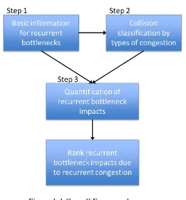
Figure 1-1 Overall Framework
This thesis is conducted following the depicted framework shown in Figure 1-1.
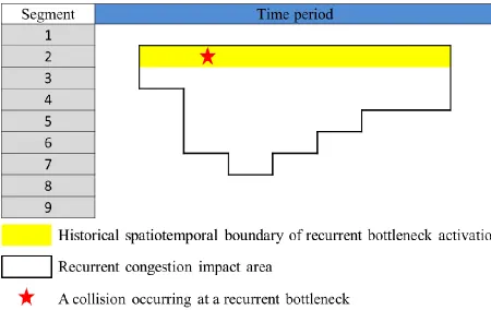
Figure 1-2 illustrates what is planned to be executed throughout the research. In the figure,
the yellow box denotes a historical spatiotemporal bottleneck activation area. The red star
drawn in the figure depicts the historical recurrent congestion-impacted area due to an active
bottleneck.
Figure 1-2 Spatiotemporal Traffic State Matrix for Key Tasks
1.2 Research Scope
Most traffic data used in this thesis were obtained through by the Regional Integrated
Transportation Information System (RITIS) operated by the University of Maryland CATT
Lab. For the collision classification, crash data were gathered from Traffic Engineering
Accident Analysis System (TEAAS) provided by North Carolina Department of
Transportation.
All methodologies presented here were developed based on heuristic methods using
areas. However, it should be noted that both public agencies and researchers should clarify
and understand their own regional unique characteristics of recurrent bottlenecks and crashes.
1.3 Research Contribution
This thesis presents a comprehensive understanding of freeway recurrent bottleneck
and its impact area to researchers or agencies who are interested in analyzing freeway
bottlenecks. Many studies have been conducted on bottleneck identification and
understanding spatiotemporal characteristics. However, this research is unique from other
studies in several ways in that it.
Defines recurrent bottleneck locations with time span of bottleneck activation
based on long-term temporal link speed data;
Provides novel and defensible definition of recurrent and non-recurrent
congestion;
Classifies congestion types when crashes occur; and,
Distinguishes and quantifies recurrent congestion impact separated from
collision-induced congestion impact.
The results of the research proposed will support decision makers in their efforts to
implement mobility, reliability, and safety treatments that are precisely targeted and
effective.
1.4 Organization of the Thesis
This thesis consists of seven chapters. In the next Chapter a literature review on
chapter also introduces a novel concept of the definition of recurrent congestion. Chapter
Five presents a comprehensive collision classification methodology. This is based on the
result of recurrent bottleneck identification. Chapter Six provides a data-driven approach for
quantifying spatiotemporal recurrent congestion impacts. Chapter Seven finally provides a
summary of the research results, including findings, conclusions, and future
LITERATURE REVIEW
Many studies have been defined and identified congestion by using the concepts of
breakdown, bottleneck, and congestion, and in fact they used these concepts interchangeably.
This calls for a thorough review on them. To define and identify recurrent bottleneck, a
literature review for distinguishing between recurrent and non-recurrent congestion is the key
to classify congestion types of which crashes occur. With the background, the literature
review in this study focuses on the definition and identification of congestion, bottleneck,
breakdown, recurrent congestion, and secondary incident.
The first section of this literature review concerns the definition of congestion by
exploring various congestion identification methods in numerous studies. Many times, each
study had its own definition for congestion and tried to identify congestion under the
definition. The second section is about distinguishing recurrent and non-recurrent congestion.
Most studies also had their own definition of the classification methodology. The third
section is about the secondary incident identification methods by exploring previous studies.
The final section is about approaches for quantifying bottleneck impacts.
2.1 Traditional Congestion and Bottleneck Identification
There are three major concepts in identifying congestion conditions: “congestion”,
“breakdown”, and “bottleneck”. These are obviously different concepts and definitions, but
many studies have been conducted using a single definition alone. Therefore, these are
2.1.1 Breakdown
The “breakdown” phenomenon is defined as a traffic transition state to congested
states from free flow states conditions. There are two approaches to define and identify
breakdown points: speed-based and other definitions such as occupancy-based. Previous
studies using speed-based definitions of breakdown were based on either a pre-specified
speed threshold or a precipitous speed drop. Elefteriadou et al. proposed that the average
speed threshold of all lanes on a freeway be dropped below 56 mph for a period of at least
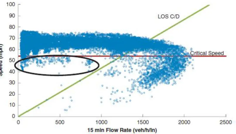
five minutes (Elefteriadou 1995). Another study by Jia et al. (2010) developed a
methodology to identify the breakdown phenomenon by applying a combination speed and
density thresholds: 1) the observed speed is below the critical speed (different value on
freeways); 2) the observed density is greater than or equal to the boundary between level of
service C and C (LOS C/D). Figure 2-1 shows a schematic combination speed and density
threshold. This method was proposed to filter points out in the black circle area in the figure.
Breakdown was referred to as the points below the red line of critical speed and to the right
of the LOS C/D line.
In addition to speed-based definition of breakdown, several studies have proposed an
alternative definition of breakdown, especially which of sudden occupancy increase over
flow rate. Hall and Agyemang-Duah used a ratio of the occupancy over flow rate as the
breakdown indicator. In this study, a ratio of 1.1 was used as the threshold (Hall and
Agyemang-Duah 1991). Zhang and Levinson also used a threshold of occupancy as the
indicator of breakdown. If the occupancy from a detector is larger than 25%, this station is
Manual 2010 (TRB 2010) defines a segment as having an equal or greater than 1 ratio of
demand/capacity.
Figure 2-1 Critical Speed and LOS C/D on I-880 Speed Flow Data (Jia et al. 2010)
2.1.2 Bottleneck
A traffic “bottleneck” is well known as a “physical bottleneck” and is usually defined
as any location where there is a physical reduction in the roadway width, such as lane drops.
Neudorff et al. defined bottleneck as a short segment of highway with insufficient capacity
(Neudorff et al. 2011). Although bottleneck is usually defined as a physical location, several studies have developed bottleneck identification methodologies with no distinction between
2
j i
x x miles Equation 2-1
,
( k ) ( , )l 0 i k l j
v x t v x t if x x x x Equation 2-2
( j, ) ( , )i 20
v x t v x t mph Equation 2-3
( , )i 40
v x t mph Equation 2-4
Location xi is upstream of xj, xk, xl are the detectors between these locations. If the
above four inequalities hold, there is an active bottleneck between two locations, xj, xi, with xi
< xj, during period t. The authors defined recurrent bottleneck with the following equation:
1
1 2
( ) , 1
t N i r t
A qN t t t N
Equation 2-5Where Ai(t) = 1, if there is an active bottleneck at location i in time period t. In this
study a recurrent bottleneck is defined as a sustained bottleneck if there are at least several
active bottlenecks periods (or 25 minutes) within specified consecutive periods (or 1 hour),
N.
Warita et al. exhibited a method for identifying potential bottlenecks along with
freeways. The ratio (85th percentile) of free-flow speed was selected as the threshold of
bottleneck occurrence (Warita et al. 2006). However, the threshold value for determining bottlenecks was not clearly specified in this study. Although a case study was performed
using 5-minute speed data collected from Tokyo metropolitan expressway, the accuracy of
the result was not well justified.
Wiezorek et al. conducted a rigorous evaluation of a previous bottleneck
identification method proposed by Chen et al. (Chen et al. 2004), in which a bottleneck was declared if the speed at upstream detectors was below the maximum upstream speed
MinSpeedDifferential) (Wieczorek 2010). This study conducted a sensitivity analysis to
adjust the three parameters in Chen’s model (MaxUpstreamSpeed, MinSpeedDifferential,
and Aggregation Interval) to achieve the best model performance. Using the sensitivity
analysis model, five values of each parameter in a total of 125 combinations were tested
using the archived dataset of the northbound I-5 corridor in Portland, Oregon. For
comparison purposes, 91 bottlenecks over 24 days were extracted manually (and visually)
using the oblique-curve method and were set as the baseline reference points for evaluating
the outcomes of Chen’s approach. To account for the impacts of each parameter as well as
the interactions between parameters, the analysis of variance (ANOVA) model was
performed independently for each of the three score functions (SumScore, ProductScore, and
Accuracy). Consequently, the original parameter value in Chen’s model applied for the San
Diego (SA) data (20 mph minimum speed differential, 40 mph maximum upstream speed,
and 5-min aggregation) were close to, but not the same as, the optical settings for this
Portland freeway (15 mph differential, 35 mph maximum upstream speed, and 3-min
aggregation). The authors also recommended that, for researchers and transportation
managers in other cities wishing to implement a system using the Chen’s approach, it is
necessary to perform a similar SA procedure to determine the optimal parameter settings for
their own network. Finally, this study just introduced the historical percentile methodology to
(a) Recurrence > 25% (b) Recurrence > 40% (c) Recurrence > 75%
Figure 2-2 Bottleneck Activation Sites (with Darkness Proportional to Frequency of Recurrence) (Wieczorek 2010)
Yildirimoglu and Geroliminis presented a methodology for forecasting travel time
along a roadway segment using speed data at fixed loop detectors (Yildirimoglu and
Geroliminis 2012). In this study, the travel time prediction problem was divided into two
parts: 1) forecasting major traffic events on the roadway (e.g. bottlenecks) and 2)
determining the speed profile in the time-space diagram. A previous bottleneck identification
method proposed by Chen et al. was employed to determine the location and spatial extent of
the bottlenecks. Since a large number of detectors and time periods in a day may result in
large number of observations, the authors utilized the principal component analysis (PCA)
method to reduce the dimensions of the dataset. A probability distribution map of congestion,
established by clustering analysis, was further developed for calculating travel time. During
the second part, the speed profile inside the bottlenecks was calculated using the minimum of
instantaneous and average speed; while the travel time for non-bottleneck locations was
computed directly using instantaneous travel speed. Five-minute loop detector data, covering
a 60 mile section of I-5 in the district of the San Diego/Imperial area was extracted from the
indicated that the proposed methodology provided promising travel time predictions for
various traffic flow conditions.
Florida (2011) presented a methodology for identifying bottlenecks on Florida’s
Strategic Intermodal System (SIS) using vehicle probe data and travel time reliability
measures. The vehicle probe data, obtained from INRIX, provided travel speeds from the
roadway for an entire year at five-minute intervals. To identify bottlenecks at the statewide
and districtwide level, this study employed two TTR measures: 1) planning time index (PTI)
and 2) frequency of congestion (FOC). The frequency of congestion is defined as the percent
of time that travel speeds fall below 75% of the free-flow speed during the daytime.
Bottlenecks were identified as the portion of the congested roadway which has the highest
combination of PTI and FOC with Figure 2-3. The proposed can be updated annually with
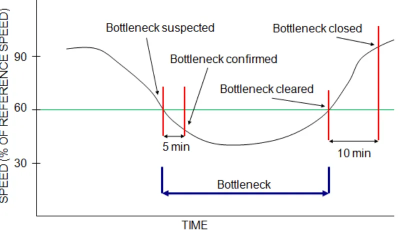
The Vehicle Probe Project Suite provides bottleneck ranking (RITIS 2016) by
defining and identifying bottlenecks as a Traffic Message Channel (TMC)’s speed goes
below 60 percent of the free-flow speed as seen in Figure 2-4. In contrast to other bottleneck
activation algorithms discussed above, the potential bottleneck suspected is used if speed at a
TMC segment drops below the reference speed of that segment and if that speed is
maintained for at least 5 minutes. This method declares a termination of bottleneck if the
speed rises above the reference speed and that continues for at least 10 minutes.
2.2 Recurrent Congestion Versus Non-Recurrent Congestion
Traffic congestion can be classified as either recurrent or non-recurrent. A consensus
about the definition of non-recurrent congestion is any unexpected delay caused by an
incident, a work zone, adverse weather, and so forth (Hallenbeck et al. 2003, Skabardonis et al. 2003, Kwon et al. 2006, Medina 2010, Chung 2011, Sullivian et al. 2013). However, a variety of definitions exists for recurrent congestion. For instance, Caltrans (2016) defined
recurrent congestion as when the average speed drops below 35 miles per hour for 15
minutes or more on a typical weekday on a freeway. Schaefer considered a value of 1.5 for
the Travel Time Index (TTI) as being the threshold of recurrent congestion (Schaefer et al. 2011). Dowling et al. defined recurrent congestion as being caused by demand surges or
capacity deficiencies in peak periods (Dowling et al. 2004).
A study by Hallenbeck et al. defined non-recurrent congestion and then associated
any congestion not within those non-recurrent congestions’ characteristics as recurrent
congestion (Hallenbeck et al. 2003). The non-recurrent congestion in the study was defined as a condition where the lane occupancy is 5 or more percentage points higher than the
median for all days during the period of interest.
Another study by Medina (2010) developed a method to distinguish non-recurrent
and recurrent congestion based on delay threshold using loop detector data as seen in Figure
2-5. This study introduced the concept of “recurrent”. In this study, ‘recurrent congestion
segments’ (RCS) with delays on 50% or more of the days during a specified period were
recurrent delays, it moves on to step 11 to check network effects. If there is no problem with
network effects, then the incident is finally classified as another cause of non-recurrent delay.
Figure 2-5 Methodology to Assess Recurrent and Non-recurrent Congestion (Medina 2010)
Skabardonis et al. used the average and the probability distribution of delays to
delay in the absence of those incidents. Thus, total delay is the sum of non-recurrent
congestion and recurrent congestion.
Chung defined non-recurrent traffic congestion as the extra delay caused by incidents
compared with the annual average section travel speed (Chung 2011). For instance, if the
free-flow speed is 60 mph and the annual average section travel speed is 30 mph during peak
periods, then it is assumed that recurrent congestion occurs. In the study, the difference the
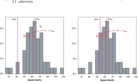
mean speed 𝑠̅𝑖(𝑡𝑚) and the threshold, 𝛼 ∙ 𝜎𝑠𝑖(𝑡𝑚), where 𝛼 is a positive value, any particular
speed 𝑠̂𝑖(𝑡𝑚), mean speed 𝑠̅𝑖(𝑡𝑚), and standard deviation speed 𝜎𝑠𝑖(𝑡𝑚) was drawn from the
distribution of 𝑠𝑖𝑛(𝑡𝑚), respectively. On the basis of such results, two discriminatory values
as seen in Figure 2-6 can be assigned to all cells representing the speed 𝑠̂𝑖(𝑡𝑚) as follows:
( )
ˆ
0 ( ) ( )
( ) 1
m
i m i m si t i m
if s t s t D t
otherwise
In recent, there was one study (Sullivian et al. 2013) which used the link based speed data (the INRIX Traffic Message Channel data) for defining recurrent and non-recurrent
congestion. The Standard Normal Deviate (SND) procedure, which was first proposed by
(Dudek et al. 1974), was used to distinguish recurrent and non-recurrent congestion. The SND for each speed was calculated as shown in the following equation:
ˆ | it i|
it
u u
SND
SD
Equation 2-7
Where,
SND: standard normal deviate;
i/t: number of row/column respectively; ˆit
u : speed at segment i in time t;
i
u : average speed at segment i during the specified time period T(T
t ); and, SD: standard deviation.This procedure allows users to scan historical speed data, identify congestion, and
characterize them as either recurrent or non-recurrent with 4 threshold values between -1.3
and -1.9.
Previous studies use either the mean or the median of a speed distribution during a
specified time of day to measure recurrent delay and extra delay caused by incidents as
non-recurrent congestion on a freeway. However, Oxford’s Dictionary defines “non-recurrent” as
being something that occurs often or repeatedly. In other words, recurrent congestion means
a “predictable” location with time and when drivers fell like “this area on this time is often
2.3 Secondary Crash
In this thesis, crashes which occur in non-recurrent congestion locations are classified
as such. This definition approximates that of a secondary crash as found in the literature. In
other words, this type of crash classification can be referred to as a secondary crash by
crashes that occur during a non-recurrent congestion period. Thus, classification of crashes in
a non-recurrent congestion need further investigated methodologies to identify secondary
crashes. Previous regarding studies for identifying secondary crashes were two folds: 1)
secondary crash or incident identification and 2) major factors associated with such a crash.
This literature review focused on the previous one for the purpose of this thesis.
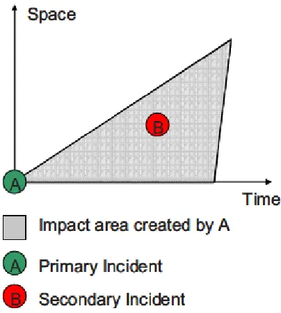
The key to identifying secondary crashes is to determine the boundaries of the
primary incident area as seen in Figure 2-7, since secondary incidents (crashes) are defined
The methodologies used either static or dynamic thresholds to determine the
boundaries of a primary incident impact area. Static thresholds employ a fixed boundary. For
example, if an incident occurs within 15 minutes and 1 mile upstream of a primary incident,
it is classified as a secondary incident, assuming these values meet the thresholds (Raub
1997a). Moore et al. identified secondary incidents as those that occur within two hours and
two miles of a primary incident using California (CA) Highway Patrol data sources (Moore
et al. 2004). The study found that the frequency of secondary crashes is about 1.5% to 3% to that of primary crashes. However, the primary incident impact area can actually be longer
than the fixed threshold boundaries.
Methodologies that use dynamic thresholds can overcome some of the limitations of
static approaches. In 2007, Sun and Chilukuri developed a dynamic threshold method by
varying the back of a queue location throughout the entire duration of the incident (Sun and
Chilukuri 2007). This study indicates that by using a dynamic approach up to a 30%
difference can arise in the number of incidents classified as secondary. Chou and
Miller-Hooks proposed a simulation-based secondary incident filtering method (SBSIF) using the
CORSIM microscopic simulation tool (Chou and Miller-Hooks 2010). They implemented a
regression model for corner point identification of the boundaries of the primary incident
impact area along with the SBSIF method. In another research study performed in Virginia,
Zhang and Khattak analyzed the cascading incident event duration (Zhang and Khattak
2010a). They identified and analyzed not only single-pair events (one primary and one
secondary incident) but also large-scale events (one primary and multiple secondary
incidents) by categorizing them as either contained or extended, using deterministic queueing
such an event, it is considered an extended event; otherwise, it is classified as a contained
event. Later they developed an incident management integration tool to calculate dynamic
incident duration predictions, secondary incident occurrences, and incident delays (Khattak et al. 2012).
Recently, Chung introduced a procedure to identify secondary crashes by different
types of primary crashes in the impact area and developed a method to separate the
non-recurrent congestion from any non-recurrent congestion using inductive loop detector data
(Chung 2013). Yang et al. proposed the use of historical virtual sensor measurements to
identify secondary crashes using a Representative Speed Contour Map (RSCP) with
percentile speed of historical incident-free virtual sensor speed measurements of each
spatiotemporal cell (Yang et al. 2013). Using the measurements, the study tried to show recurrent congestion areas and non-recurrent congestion areas in a speed contour map only
with the RSCP. However, to appropriately find the precise recurrent congestion area, the
bottleneck point needs to be identified first. In addition, the distribution of speed collected
from detectors did not follow a specified distribution. Therefore, it is hard to determine a
representative historical speed. Table 2-1 shows the comparison of secondary incident
identification from previous studies.
Most of the studies used point detector data, such as inductive loop detectors and
overhead or side fire radar detectors. However, an in-depth examination of secondary crashes
requires high-resolution traffic data and more accurate incident records to identify primary
Table 2-1 Comparison of Secondary Incidents Identification Studies Study Thresholds for determining congested impact boundary
Method for determining congested impact area
Event type considered Occurrence rate of secondary incident (direction)
(Raub 1997a) Fixed 15 min. and 1 mile Crash 15.5%
(same)
(Karlaftis et al.
1999) Fixed 15 min. and 1 mile Crash 35% (same)
(Moore et al. 2004) Fixed 2 hours and 2 miles Incident 1.5~3% (same) (Hirunyanitiwattana
and Mattingly 2006)
Fixed 1 hour and 2 miles Crash 4.4%
(same)
(Zhan et al. 2009) Dynamic
Maximum queue and dissipation time of the potential lane-blockage
primary incident
Crash 3.23%
(same)
(Chou and
Miller-Hooks 2010) Dynamic
A regression model for corner point identification of primary
incident boundary
Incident 15% (same)
(Vlahogianni et al.
2010) Dynamic
A Bayesian network model using the characteristics of primary
incident
Crash 16% (same)
(Zhang and Khattak
2010a) Dynamic
Queue-based secondary
incidents identification Incident
2.7 (same), 0.38 (opposite)
(Chung 2013) Dynamic
Binary speed contour plot on a representative speed contour map when
a crash occurs
Crash
8.1 (same), 3.7 (opposite)
(Yang et al. 2013) Dynamic
Congestion speed contour plot on a representative speed contour plot when a crash
occurs
Crash 8.42%
2.4 Quantification of Bottleneck Impact
There have been a few studies related to quantifying bottleneck impacts. In the RITIS
database, a dashboard is provided for bottleneck ranking (RITIS 2016). The bottleneck
ranking method quantifies bottleneck by an impact factor, which is the product of average
duration, average maximum length of queue, and number of bottleneck occurrences for a
given period of time on a given TMC per the follow equation:
IF D L O Equation 2-8
Where,
IF: impact factor
D: average duration (minutes)
L: average maximum length of queue (miles) O: number of occurrences
Another study by Liu and Fei (2010) proposed a fuzzy-logic-based approach that can
diagnose the severity of bottleneck based on travel delay and frequency. This approach used
Figure 2-8 Linguistic State Space and Rules of the Bottleneck Severity Diagnosis (Liu and Fei 2010)
There are several limitations to those approaches. In order to quantify and rank
bottlenecks properly, the head of the recurrent bottleneck should be identified first. However,
those approaches rank and quantifies all segments with no attempt to identifying the
bottleneck head location, which is critical to identifying problem area. In addition, those
approaches quantify impact factors without separating the additional congestion impacts due
world, there is always a probability that those same bottlenecks can be exacerbated when
there is a crash within their area of impact. The above methods may overestimate the impact
factor.
2.5 Summary
Extensive literature reviews were mainly focused on four areas: breakdown and
bottleneck identification, distinguishing between recurrent and non-recurrent congestion,
secondary crash identification, and quantification of bottleneck impact. Some of the major
findings are summarized as follow:
The definition of congestion and its identification method should be clearly
defined because the same field data would be likely produce much different
congestion values.
There is no detailed definition and identification of “recurrent bottleneck”.
Therefore, the “recurrent bottleneck” should be clearly defined in real
“recurrent” terms, where congestion occurs repeatedly in specified time
periods.
The use of a threshold from a speed distribution for each spatiotemporal cell
in defining “recurrent congestion” is improper because the cells have
different speed distribution. Therefore, it is hard to apply to distinguishing
recurrent and non-recurrent congestion. Although a speed distribution is used
to distinguish recurrent and non-recurrent congestion, we cannot say whether
using the point-based data is elusive when determining congestion boundaries
from the data collection points.
There is no crash classification under operational conditions.
It is imperative that recurrent congestion and additional congestion due to an
incident occurring within a spatiotemporal historical bottleneck impact area
should be identified and quantified separately when it comes to identifying
DATA-DRIVEN SPATIOTEMPORAL “RECURRENT”
BOTTLENECK IDENTIFICATION
3.1 Introduction
Traffic congestion and safety issues are increasingly contributing to major challenge
for transportation agencies as populations grow, motorization increases, and population
densities change. Congestion is contributing to longer travel time, higher fuel consumption,
and increased emissions of air pollutants. Nearly 40% of roadway congestion in the United
States stems from recurrent bottlenecks (Cooner 2011), which can cost both agencies time
and money if not properly addressed. Agencies should therefore identify and understand
where and when congestion occurs recurrently.
Although an active bottleneck is “a physical point on the network upstream of which
one finds a queue and downstream of which one finds freely flowing traffic” (Bertini and
Leal 2005), most studies have focused on identifying congestion with no attention to
distinguishing recurrence level of at the same “bottleneck” location. In the real world, it is
likely that several bottlenecks can be activated within a congestion-impacted area.
Accordingly, the detailed spatial and temporal characteristics of bottlenecks should be first
identified in order to quantify and diagnose a bottleneck and its impact area.
This chapter introduces an easily implementable methodology for identifying
definition of “recurrent” bottlenecks. The findings from this study can help decision makers
better prioritize investment in current facilities and/or develop suitable strategies to alleviate
congestion.
In the remainder of this chapter, a review of relevant literature is presented followed
by the methodology. In the next section, the methodology was applied to statewide interstates
of North Carolina. Finally, findings and recommendations for further research are discussed.
3.2 Review of Relevant Studies
3.2.1 Bottleneck, Breakdown, and Congestion Definitions
The “breakdown” phenomenon is typically defined as a traffic transition from a free
flow state to a congested state. The two approaches most frequently used to define and
identify breakdown are based and occupancy-based. Previous studies using
speed-based definitions select either a pre-specified speed (Lorenz 2001, Jia et al. 2010) or a precipitous speed drop threshold (Elefteriadou 1995, Brilon 2005). Other studies have
proposed an alternative definition of breakdown phenomenon (Hall and Agyemang-Duah
1991, Zhang and Levison 2004), based on the rate of occupancy increase with flow rate.
Various approaches were developed for identifying bottlenecks using point-based
detector and probe vehicle data. Chen et al. (2004) developed an algorithm for identifying
locations at activate time. In this study, a bottleneck was activated if the speed at upstream
detectors dropped below a cut-off upstream speed threshold and the speed difference between
upstream and downstream detectors was above a cut-off speed difference threshold. The
study also defined recurrent bottleneck as a sustained bottleneck if there were at least several
active bottleneck periods (e.g. 25 minutes) within specified consecutive periods (e.g. 1 hour).
other application (Liu and Fei 2010, Wieczorek 2010, Yildirimoglu and Geroliminis 2012).
For instance, Wieczorek et al. (2010) conducted a sensitivity analysis to adjust the cut-off
speed values in the Chen et al.’s method.
In recent years, probe vehicle data has been used to identify bottleneck locations. For
example, researchers in Florida (2011) developed a methodology for identifying bottlenecks
on Florida’s Strategic Intermodal System (SIS). Using travel time reliability measures that
include the planning time index (PTI) and the frequency of congestion (FOC). The latter was
defined as the fraction of time that travel speeds are below 75% of the free-flow speed in
daytime. Bottlenecks were identified as the links or the congested roadway which has the
highest combination of PTI and FOC. INRIX bottleneck ranking method defines bottlenecks
as a condition when a Traffic Message Channel (TMC)’s speed falls below 60% of the
reference speed for at least 5 minutes (INRIX 2016). The method declares a bottleneck
cleared if the speed recovers above the reference speed for at least 10 minutes. Although a
traffic “bottleneck” is well known as a “physical bottleneck”, usually any location where
there is a capacity reduction that causes congestion, many of the studies have used bottleneck
and congestion identification interchangeably. Recently, Hale et al. (2015) developed a
congestion and bottleneck identification tool. In the tool, congestion was identified using
cut-off speed values which the user can select using their own definition.
3.2.2 Recurrent Congestion
Traffic congestion can be classified into two types: recurrent and non-recurrent
literature currently lacks a robust definition for recurrent congestion. Rather, authors have
historically identified recurrent congestion based on their own definition for the purpose of
their studies. For instance, Medina (2010) deems a segment with delays on 50% or more of
the days during a specified period is defined to have recurrent congestion. Another study by
Hallenbeck et al. (2003) defined the median for all days during the period of interest.
Skabardonis et al. (2003) defined recurrent congestion as the delay in absence of incidents.
Recurrent congestion by Chung (2011) is referred as the difference between free flow speed
and the annual average section travel speed during peak periods.
Very often, previous studies used parameters from the speed distribution in a time
window of day to distinguish recurrent congestion from non-recurrent congestion. Under this
paradigm, bottlenecks on rural roads, which means that any congestion detected would be
classified as non-recurrent.
Given these circumstances, this study develops an easily implementable approach for
identifying recurrent bottleneck location with time, which does not require speed distribution
to distinguish recurrent and non-recurrent congestion.
3.3 Methodology
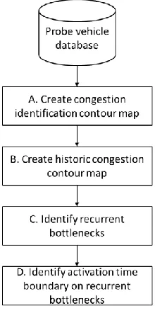
3.3.1 Overall Framework
The overall framework is outlined in Figure 3-1. In the first step, daily congestion
identification contour maps are created for a road segment in a specified time period. The
congestion contour map created is a spatial temporal binary congestion state matrix
(congested or free flow). In the second step, a historic congestion contour map is created by
overlapping congestion identification contour maps from several days or months. The spatial
contour map in the third step. Finally, time spans of activation of the recurrent bottlenecks
are identified. The framework presented in Figure 3-1 comprises several data-driven models,
as explained next. In the remainder of this section, data sources that are used in this study are
discussed, and the further details of the proposed methodology are described.
Figure 3-1 Overall Recurrent Bottleneck Identification Framework
3.3.2 Data Source
This research used the link-based speed data generated from GPS-enabled vehicle
probes using INRIX technology (INRIX 2016). Those data can be directly downloaded from
the Regional Integrated Transportation Information System (RITIS), a database that includes
many performance measures and a user dashboard (RITIS 2016). In this study, speed and
3.3.3 Congestion Identification
3.3.3.1 Congestion, bottleneck, and breakdown phenomenon
Figure 3-2 depicts visual definition of these terms. This thesis defines “breakdown”
as a transition point from an un-congested state to a congested state. A “bottleneck” is defined as a location where congestion occurs when the ratio of demand to capacity is equal to or greater than 1 from either physical characteristics or operational conditions. Finally, this thesis defines “congestion” as a traffic condition where the speed drops below the speed at capacity on a segment.
Figure 3-2 Schematic Definition of Breakdown, Bottleneck, and Congestion
3.3.3.2 Congestion value and index
( , , )
( , , ) 100%
( ) d or w
MS i t m
C i t m
FFS i
Equation 3-1
Where,
i:TMC segment i,
t: specified time interval in a day (e.g., 8:00-8:15,15 min); typically t will vary from 1 to 96 for a single day,
m: index for a day in the study period,
d: weekday (Monday, Tuesday, Wednesday, Thursday, Friday),
w: weekend (Saturday, Sunday),
MS (i,t,m): reported speed (mi/h),
:free flow speed (mi/h) for segment (i), and
( , , )
d or w
C i t m : congestion value for segment (i) at time (t) on day m.
Although the FFS (i) of a TMC segment is provided via INRIX.com, FFS (i) could not be applied to this thesis since different FFSs (i) are reported for different time periods. Therefore, this study uses the simple model for predicting free flow speed on a highway
segment developed by the Florida DOT (Moses 2013), in which FFS (i), is simply calculated by adding 5 mph to the posted speed limit on a TMC segment. If Cd or w( , , m)i t is below a
cut-off speed threshold, 𝛼, the TMC segment i is considered to be congested at time t during day m. The congestion index, CId or w( , , m)i t , based on Cd or w( , , m)i t is defined as follows:
( )
Where,
( , , m)
d or w
CI i t : Congestion Index at a spatiotemporal traffic state matrix (STM) (i,t) and all other variables as defined earlier.
Figure 3-3 depicts a schematic congestion index contour map on Northbound I-85 in
NC on January 3, 2014. In this study, is estimated with the ratio of speed at capacity to
free flow speed in the latest version of the US Highway Capacity Manual (TRB 2010). For
instance, 80% of the cut-off speed threshold can be applied to the TMC where the posted
speed limit is 60 mph (i.e. free flow speed is 65 mph).
Figure 3-3 Congestion Index Contour Map (3 January 2014, on I-85 Southbound)
3.3.4 Average Historic Congestion Index
The Average Historic Congestion Index, AHCId or w( , )i t , is a key parameter for
identifying a “recurrent” bottleneck. It is defined as the fraction of days in the reporting
period T (typically one or more years) where a TMC segment i was congested at time t, based on the specified congestion index, (CId or w( , , ))i t m :
4:15 PM 4:30 PM 4:45 PM 5:00 PM 5:15 PM 5:30 PM 5:45 PM 6:00 PM 6:15 PM 6:30 PM
125-04627 I-85 SOUTHBOUND GASTON 0.41 0 0 0 0 0 0 0 0 0 0
125N04628 I-85 SOUTHBOUND GASTON 0.39 0 1 1 1 0 0 0 0 0 0
125-04628 I-85 SOUTHBOUND GASTON 2.15 0 1 1 1 1 1 1 1 0 0
125N04629 I-85 SOUTHBOUND GASTON 0.29 0 1 1 1 1 1 1 1 1 0
125-04629 I-85 SOUTHBOUND GASTON 0.72 0 1 1 1 1 1 1 1 1 0
125N04630 I-85 SOUTHBOUND GASTON 0.63 0 0 1 1 1 1 1 1 1 0
125-04630 I-85 SOUTHBOUND GASTON 2.01 0 0 1 1 1 1 1 1 1 0
125N04631 I-85 SOUTHBOUND MECKLENBURG 0.81 0 0 0 1 1 1 1 0 0 0
125-04631 I-85 SOUTHBOUND MECKLENBURG 0.02 0 0 0 0 0 1 0 0 0 0
125N04632 I-85 SOUTHBOUND MECKLENBURG 0.63 0 0 0 0 0 0 0 0 0 0
TMCcode On Road Direction County Length (miles) Time
1
( , , )
( , ) 100(%)
M d or w m
d or w
CI i t m
AHCI i t
M
Equation 3-3Where,
M: the number of days in the study period (e.g. 250 weekdays in a year) : Average Historic Congestion Index at for segment i at time t.
The AHCI proposed represents the probability that TMC segment i is congested at time interval t over M days of observation. For instance, Figure 3-4 shows that the
probability of congestion for TMC 125+04965 at 7:30 AM in 2014 was 85%. An AHCI
value of 20% or more would indicate congestion occurring on average more than a day a
week (excluding weekends) on segment i at time t.
( , ) d or w
3.3.4.1 Spatial patterns of AHCI
This thesis identifies recurrent bottlenecks based on the AHCI contour map.
Therefore, the first step for identifying recurrent bottlenecks is to ascertain the
spatiotemporal characteristics of the AHCI contour map. The question then is which TMCs is
identified as a recurrent bottleneck?
To answer the question, the author identified three different spatial patterns observed
on weekdays in 2014 on all Interstates in North Carolina. Figure 3-5 describes the patterns
that are directly applicable to recurrent bottleneck identification.
The TMCs identified as a recurrent bottleneck usually have the highest AHCI (TMC
A as seen in Site 1 of Figure 3-5 (a)) and are located just upstream of a significant drop in
AHCI value. Therefore, these TMCs are clearly defined as recurrent bottleneck segments and
are labeled as Spatial Pattern 1 in this study.
Different spatial patterns were associated with other recurrent bottlenecks in the
AHCI contour map. Site 2, shown in Figure 3-5 (b), exhibits a pattern of AHCI where the
TMC with the highest AHCI value (TMC C) is not located immediately upstream of a
significant drop in AHCI. In this case, TMC C and the one downstream of it (TMC B) have
AHCI values greater than 90% and TMC B is located upstream of a significant drop in
AHCI. Therefore, TMC C is also part of the bottleneck and this pattern is called as Spatial
Pattern 2. If the “physical” recurrent bottlenecks are located nearly at the end of TMC B and
adjacent downstream of TMC C, the TMC B may report a travel speed based on mixed
traffic flow. In this case, the AHCI value at TMC B may be lower than that at TMC C.
In Figure 3-5 (c), Site 3 describes the final spatial pattern detected in this research. No
TMCs with AHCI greater than % (e.g. 50% is for Figure 3-5 (c)) are referred as recurrent
bottlenecks, only TMC D can be included in a recurrent bottleneck. This conditions labeled
(a) Spatial pattern 1 of AHCI (Site 1 - 125+04965 on I-40 Westbound in Wake County, NC)
(b) Spatial pattern 2 of AHCI (Site 2 - 125N04663 on I-485 Counterclockwise in Mecklenburg County, NC)
(c) Spatial pattern 3 of AHCI (Site 3 - 125+04860 on I-40 Westbound in Wake County, NC)
Figure 3-5 Spatial Patterns of AHCI in 2014
3.3.4.2 Temporal patterns of AHCI
impact area corresponding to Figure 3-5. Figure 3-6 (a) shows AHCI values exhibiting a bell
shape curve over time. AHCIs’ at 7:45 AM were at the highest values during congested
conditions, then decreased gradually over time. This trend is labeled Temporal Pattern 1.
Figure 3-6 (b) shows a slightly different temporal pattern. Several TMCs had AHCI values
greater than 80% for 90 minutes, and then decreased sharply and this pattern is labeled
Temporal Pattern 2. In Figure 3-6 (c) AHCI values on TMCs increased and then decreased
slowly without any significant drop. However, the AHCI values where TMCs have greater
than 50% appear similar to Temporal Pattern 1. It indicates that no difference between (a)
and (c) of Figure 3-6 was found. Therefore, two temporal patterns were finally identified for
(a) Site 1
(b) Site 2
(c) Site 3