FAC-PIN: An efficient and fast agglomerative clustering algorithm for protein interaction networks to predict protein complexes and functional modules

(1)

Scholarship at UWindsor

Electronic Theses and Dissertations Theses, Dissertations, and Major Papers

2013

FAC-PIN: An efficient and fast agglomerative clustering algorithm

for protein interaction networks to predict protein complexes and

functional modules

Mohammad Shamsur Rahman University of Windsor

Follow this and additional works at: https://scholar.uwindsor.ca/etd

Recommended Citation Recommended Citation

Rahman, Mohammad Shamsur, "FAC-PIN: An efficient and fast agglomerative clustering algorithm for protein interaction networks to predict protein complexes and functional modules" (2013). Electronic Theses and Dissertations. 4859.

https://scholar.uwindsor.ca/etd/4859

This online database contains the full-text of PhD dissertations and Masters’ theses of University of Windsor students from 1954 forward. These documents are made available for personal study and research purposes only, in accordance with the Canadian Copyright Act and the Creative Commons license—CC BY-NC-ND (Attribution, Non-Commercial, No Derivative Works). Under this license, works must always be attributed to the copyright holder (original author), cannot be used for any commercial purposes, and may not be altered. Any other use would require the permission of the copyright holder. Students may inquire about withdrawing their dissertation and/or thesis from this database. For additional inquiries, please contact the repository administrator via email

(2)

NETWORKS TO PREDICT PROTEIN COMPLEXES AND

FUNCTIONAL MODULES.

by

MOHAMMAD SHAMSUR RAHMAN

A Thesis

Submitted to the Faculty of Graduate Studies

through the School of Computer Science

in Partial Fulfillment of the Requirements for

the Degree of Master of Science at the

University of Windsor

Windsor, Ontario, Canada

2013

c

(3)

NETWORKS TO PREDICT PROTEIN COMPLEXES AND

FUNCTIONAL MODULES.

by

MOHAMMAD SHAMSUR RAHMAN

APPROVED BY:

Dr. Abdulkadir Hussein, External Reader Department of Mathematics and Statistics

Dr. Luis Rueda, Internal Reader

School of Computer Science

Dr. Alioune Ngom, Advisor

Dr. Christie Ezeife, Chair of Defense

(4)

I hereby certify that I am the sole author of this thesis and that no part of this thesis has

been published or submitted for publication.

I certify that, to the best of my knowledge, my thesis does not infringe upon anyone’s

copyright nor violate any proprietary rights and that any ideas, techniques, quotations, or

any other material from the work of other people included in my thesis, published or

oth-erwise, are fully acknowledged in accordance with the standard referencing practices.

Fur-thermore, to the extent that I have included copyrighted material that surpasses the bounds

of fair dealing within the meaning of the Canada Copyright Act, I certify that I have

ob-tained a written permission from the copyright owner(s) to include such material(s) in my

thesis and have included copies of such copyright clearances to my appendix.

I declare that this is a true copy of my thesis, including any final revisions, as approved

by my thesis committee and the Graduate Studies office, and that this thesis has not been

submitted for a higher degree to any other University or Institution.

(5)

Proteins are known to interact with each other to perform specific living organism functions

by forming functional modules or protein complexes. Many community detection

meth-ods have been devised for the discovery of functional modules or protein complexes in

protein interaction networks. One common problem in current agglomerative community

detection approaches is that vertices with just one neighbor are often classified as

sepa-rated clusters, which does not make sense for module or complex identification. In this

thesis, we propose a new agglomerative algorithm, FAC-PIN, based on a local premetric

of relative vertex-to-vertex clustering value. Our proposed FAC-PIN method is applied

to PINs from different species for validating functional modules and protein complexes

generated from FAC-PIN with experimentally verified functional modules and complexes

respectively. The preliminary computational results show that FAC-PIN can discover

func-tional modules and protein complexes from PINs more accurately. As well as we have

also compared the computational times for different species with HC-PIN and CNM

algo-rithms. Our algorithm outperforms two algoalgo-rithms. Our FAC-PIN algorithm is faster and

accurate algorithm which is the current state-of-the-art agglomerative approach to complex

prediction and functional module identification.

(6)

I would like to dedicate this thesis to my creator and Everlasting true Almighty Allah. My

parents and wife always want to see me reaching the highest levels of success. I am very

happy today that I am able to make them proud. Also thanks to my parent and wife for all

their prayers. It is because of their good wishes, I am able to do this research work.

(7)

I would like to take this opportunity to express my sincere gratitude to Dr. Alioune Ngom,

my supervisor, for his steady encouragement, patient guidance and enlightening

discus-sions throughout my graduate studies. Without his help, the work presented here would

have not been possible. Dr. Alioune Ngom will always remain like a father figure to me.

I also wish to express my appreciation to Dr. Christie Ezeife, Dr. Luis Rueda, School of

Computer Science and Dr. Abdulkadir Hussein, Department of Mathematics and Statistics

for being in the committee and spending their valuable time.

(8)

Author’s Declaration of Originality iii

Abstract iv

Dedication v

Acknowledgements vi

List of Figures x

List of Tables xii

1 Introduction 1

1.1 Background . . . 1

1.1.1 Protein . . . 1

1.1.2 Protein complex and Functional Modules . . . 4

1.1.3 Protein Interaction Networks . . . 5

1.1.4 Community . . . 7

1.1.5 Community Detection Algorithm . . . 10

1.2 Objectives . . . 12

(9)

1.3 Thesis Organization . . . 13

2 Relative Works 15 2.1 Density based methods . . . 15

2.1.1 Spirin et al 2003 . . . 16

2.1.2 Li et al. 2006 . . . 16

2.1.3 Altaf et al. 2006 . . . 17

2.1.4 Pei et al. 2007 . . . 18

2.1.5 Summary . . . 19

2.2 Graph partitioning approaches . . . 20

2.2.1 Dongen 2000 . . . 20

2.2.2 King et al. 2004 . . . 20

2.2.3 Graph Entropy Algorithm . . . 21

2.2.4 Summary . . . 22

2.3 Hierarchical based methods . . . 22

2.3.1 Ravasz et al. 2002 . . . 23

2.3.2 Girvan et al. 2002 . . . 23

2.3.3 Newman 2003 . . . 24

2.3.4 Radicchi et al 2004 . . . 25

2.3.5 Clauset et al 2004 . . . 26

2.3.6 Luo et al 2007 . . . 27

2.3.7 Li et al. 2008 . . . 27

2.3.8 Wang et al 2011 . . . 28

(10)

3 Fast Agglomerative Clustering Algorithms 31

3.1 Relative Vertex-to-Vertex Clustering Value . . . 31

3.2 The FAC-PIN Algorithm . . . 35

3.2.1 The algorithm . . . 35

3.2.2 Computational Complexity . . . 35

4 Computation experiments, results and discussions 39 4.1 Datasets . . . 40

4.2 Testing by Scoring Functions . . . 41

4.3 Protein Complex Discovery . . . 47

4.4 Functional Module Identification . . . 55

4.5 Conclusion . . . 59

5 Conclusion and future work 63

Bibliography 66

(11)

1.1 Levels of protein structures [28] . . . 2

1.2 αhelix andβsheet of secondary structure of proteins [3] . . . 3

1.3 Protein complexes of Baker’s yeast [15] . . . 5

1.4 Hyperclique pattern of functional modules in a protein complex [32] . . . . 6

1.5 Protein Interaction Network of Baker’s yeast [14] . . . 6

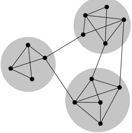
1.6 Community structure of a graphG . . . 8

1.7 Overlapping and non-overlapping communities of a graphG[23] . . . 9

1.8 Scale Free NetworkG[9] . . . 11

4.1 Modularity comparison among FAC-PIN, CNM and HC-PIN algorithms for Baker’s yeast, Cattle, Dog, E.coli, Finch bird, Flowering plant, Fruit fly and Frog . . . 43

4.2 Modularity comparison among FAC-PIN, CNM and HC-PIN algorithms for Human, Jungle fowl, Mouse, Rat, Rice, Round worm, Wild boar and Zebra fish . . . 43

4.3 -(w- log -v) comparison amongFAC-PIN,CNMandHC-PINalgorithms for Baker’s yeast, Cattle, Dog, E.coli, Finch bird, Flowering plant, Fruit fly and Frog . . . 44

(12)

4.4 -(w- log -v) comparison amongFAC-PIN,CNMandHC-PINalgorithms for

Human, Jungle fowl, Mouse, Rat, Rice, Round worm, Wild boar and Zebra

fish . . . 44

4.5 Log-log plot of execution time comparison among FAC-PIN, CNM and

HC-PINalgorithms for Baker’s yeast, Cattle, Dog, E.coli, Finch bird,

Flow-ering plant, Fruit fly and Frog . . . 45

4.6 Log-log plot of execution time comparison among FAC-PIN, CNM and

HC-PIN algorithms for Human, Jungle fowl, Mouse, Rat, Rice, Round

worm, Wild boar and Zebra fish . . . 46

4.7 Protein Interaction Network of Baker’s yeast (Y₄_K) . . . 48

4.8 Clustered Network of Baker’s yeast (Y4K) using FAC-PIN algorithm . . . . 49

4.9 Clustered Network of Baker’s yeast (Y4K) using CNM algorithm . . . 50

(13)

2.1 Summary of previous algorithms based on density based method . . . 19

2.2 Summary of previous algorithms based on graph partitioning method . . . . 22

2.3 Summary of previous algorithms based on hierarchical method . . . 29

4.1 Dataset used in experiments . . . 40

4.2 Q results of FAC-PIN, CNM and HC-PIN for Baker’s yeast, Cattle, Dog,

E.coli, Finch bird, Flowering plant, Fruit fly and Frog. . . 42

4.3 Qresults ofFAC-PIN,CNMandHC-PINfor Human, Jungle fowl, Mouse,

Rat, Rice, Round worm, Wild boar and Zebra fish. . . 42

4.4 −(w- log -)vresults ofFAC-PIN,CNMandHC-PINfor Baker’s yeast,

Cat-tle, Dog, E.coli, Finch bird, Flowering plant, Fruit fly and Frog. . . 42

4.5 −(w- log -v) results of FAC-PIN, CNM and HC-PIN for Human, Jungle

fowl, Mouse, Rat, Rice, Round worm, Wild boar and Zebra fish. . . 42

4.6 Time comparison results ofFAC-PIN,CNMandHC-PINfor Baker’s yeast,

Cattle, Dog, E.coli, Finch bird, Flowering plant, Fruit fly and Frog (in

sec-onds). . . 47

(14)

4.7 Time comparison results ofFAC-PIN,CNMandHC-PINfor Human,

Jun-gle fowl, Mouse, Rat, Rice, Round worm, Wild boar and Zebra fish (in

seconds). . . 47

4.8 Comparison of theSpecificity,SensitivityandF-score FAC-PIN,CNMand

HC-PINforBaker’s yeast. . . 54

HC-PINforHuman . . . 54

HC-PINforMouse . . . 54

HC-PINforRat . . . 55

4.12 Functional enrichment of the identified Modules which comprises of three

or more proteins ofBaker’s yeast . . . 58

4.13 Performance comparison of clustering algorithms for the identification of

large-sized (size≥20) modules ofBaker’s yeast . . . 58

small-sized (size≤6) modules ofBaker’s yeast . . . 59

4.15 Functional enrichment of the identified Modules which comprises of three

or more proteins ofRat . . . 60

large-sized (size≥20) modules ofRat . . . 60

(15)

Introduction

In the current Chapter, we discuss necessary background and the objective of the thesis. In

Section 1.1, we describe the important terminologies which help to understand the

objec-tives of the thesis. In Section 1.2, we have described the objecobjec-tives of the thesis in detail.

Finally in Section 1.3, we have shown the organization of the thesis.

1.1 Background

1.1.1 Protein

Proteins are large biological molecules consisting of multiple chains of amino acids1[28].

Proteins perform a vast array of functions within living organisms, including catalyzing

metabolic reactions, replicating DNA, responding to stimuli, and transporting molecules

from one location to another. Proteins were first described by the Dutch chemist Gerardus

Johannes Mulder and named by the Swedish chemist J ¨ons Jacob Berzelius in 1838.

1_{Amino acids are biologically important organic compounds made from amine (-NH2) and carboxylic}

acid (-COOH) functional groups, along with a side-chain specific to each amino acid

(16)

Figure 1.1: Levels of protein structures [28]

A protein having multiple chains of amino acids has four levels of structure [28]: The

four levels of the protein structure are shown in Figure 1.1. Primary structureof a protein

is the linear sequence of its amino acid structural units and partly comprises its overall

biomolecular structure [28]. The primary structure is held together by covalent or peptide

bonds, which are made during the process of protein biosynthesis2. The two ends of the

polypeptide chain are referred to as the carboxyl terminus (C-terminus) and the amino

terminus (N-terminus) based on the nature of the free group on each extremity. Counting

of residues3 always starts at the N-terminal end (-NH2 group) and ends at the C-terminal 2_{Biosynthesis is an enzyme-catalyzed process in cells of living organisms by which substrates are}

con-verted to more complex products [4]

(17)

end (-COOH group). The sequence of a protein is unique to that protein, and defines the

structure and function of the protein. The sequence of a protein can be determined by

methods such as Edman degradation4or Tandem mass spectrometry5[28]. Often however,

it is read directly from the sequence of the gene using the genetic code. There are more

than thousands types of proteins in our body which are composed of different arrangements

of 20 types of amino acid residues.

Secondary structurerefers to highly regular local sub-structures. The secondary

struc-ture consists of two major strcustruc-tures: the alpha helix (are often the basis of fibrous

poly-mers) and the beta strand or beta sheets (often has twists that increase the strength and

rigidity of the structure), were suggested in 1951 by Linus Pauling and co-workers [24].

These secondary structures are defined by patterns of hydrogen bonds between the

main-chain peptide groups. Both the alpha helix and the beta-sheet represent a way of saturating

all the hydrogen bond donors and acceptors in the peptide backbone. α helix andβsheet

of secondary structure of proteins are shown in Figure 1.2

Figure 1.2:αhelix andβsheet of secondary structure of proteins [3]

Tertiary structure of a protein is when the molecule is further folded and held in a

particular complex shape forming precise and compact structure, unique to that protein.

(18)

The shape is maintained permanently by the intra- molecular bonds:

Hydrogen bond of one hydrogen atom shared by two other atoms

Van der Waals force is the weak force that incurs when two or more atoms are very close

Disulphide bond is a strong covalent bond formed between two adjacent cysteine amino acids. The bond stabilizes the tertiary shape of a protein

Ionic bond is the electrostatic interaction between oppositely charged ions

Quaternary structureformed by several protein molecules (polypeptide chains),

usu-ally called protein subunits in this context, which function as a single protein complex.

The quaternary structure is stabilized by the same non-covalent interactions and disulphide

bonds as the tertiary structure. Quaternary structure of protein arise when a number of

ter-tiary polypeptides joined together forming a complex or time to time modules, biologically

active molecule.

1.1.2 Protein complex and Functional Modules

Protein complexare groups of proteins that interact with each other at the same time and

place, forming a single multimolecular machine [29]. These are the form of quaternary

structure of proteins. Identified protein complexes include several large transcription factor

complexes, the anaphase-promoting complex, RNA splicing and polyadenylation

machin-ery, protein export and transport complexes etc. Protein complexes of Baker’s yeast is

shown in Figure 1.3.

Functional modules are consisted of proteins that participate in a common elementary

biological process while binding each other at a different time and place (different

(19)

Figure 1.3: Protein complexes of Baker’s yeast [15]

identified functional modules including the CDK/ cyclin module responsible for cell-cycle

progression, the yeast pheromone response pathway, MAP signaling cascades etc. A 3D

structural view of hyperclique pattern of functional modules within a protein complex is

shown in Figure 1.4. It is very important to remember, functional modules contain multiple

protein complexes [5, 10]. On the other hand, protein complexes carry out a specific task,

but functional modules carry out a set of tasks which are carried out by individual protein

complexes [10].

1.1.3 Protein Interaction Networks

Network representation of proteins and their interactions are known asProteinInteraction

Network[29]. In short it is calledPIN. In PINs, proteins are represented as nodes or vertices

and interactions are as edges. Maximum PINs are undirected networks with edge weight

or not [13, 29]. In Figure 1.5, an unweighted PIN of baker’s yeast is shown.

(20)

Figure 1.4: Hyperclique pattern of functional modules in a protein complex [32]

Figure 1.5: Protein Interaction Network of Baker’s yeast [14]

interaction networks in their papers:

Small world effect which is the name given to the finding that the average distance be-tween vertices in a network is small.

Power law degree distribution is a distribution where the number of the vertices with low degree is higher than the number of vertices with high degree.

(21)

Community structure is a property where intrales or both.-connectivity of a subset of vertices of graph G is higher than inter-connectivity between others. It is briefly

discussed in Subsection 1.1.4.

Preferential attachment is a property where a new node u is likely toattach to a high-degree nodevthan to a low degree node.

In PINs, all protein complexes and functional modules are strong subgraphs6[29]. To

identify the protein complexes or functional modules from PINs means strong subgraphs,

authors of the algorithms were used any of five properties. Third and fourth properties are

commonly used to discover protein complexes or functional modules. But unfortunately,

fifth property have not still used by any authors which helps to identify the more significant

strong subgraph having biological significance.

1.1.4 Community

A community is defined as a subgraph (a subset of vertices of graphG) within the graph

G such that connections inside the subgraph are denser than connections with the rest of

the network [26]. Luo et al [21] gave the more formal definition of community. Their

definition is as

followed-Definition 1.1.1. CommunityU is a subgraph of a graph G in which in-degree of U is

higher than out-degree and the ratio of in-degree and out-degree ofU should be higher than

1.

In-degree of a communityU is the number of edges connected between the vertices

of communityU and out-degree of a communityU is the number of edges between other

(22)

communities andU. From the formal definition of community, two properties of the

com-munity are

revealed-Homogeneity: Vertices of a community are highly similar or compact to each other.

Separability: Vertices of different communities have lower similarity or compactness.

Figure 1.6: Community structure of a graphG

On the other hand, inhomogeneity or separability property suggests that the network

has certain natural divisions within it. The communities are often defined in terms of the

partition of the set of vertices, that is each node is put into either only one community just

as in the Figure 1.6 or into multiple communities. Depends on the distribution of the nodes

among the communities, community can be classified into two

(23)

communities are the examples of overlapping communities

Non-overlapping communities do not share any node between them. In Figure 1.7, blue and purple; blue and yellow colored communities do not share a single vertex

be-tween. So, these communities are the example of non-overlapping communities.

Figure 1.7: Overlapping and non-overlapping communities of a graphG[23]

In the Figure 1.7, blue and green colored communities are not connected by any edge.

These communities are known asdisjointcommunities.

Moreover, Radicchi et al. [26] also classified the communities into two groups

accord-ing their connectivities:

Strong community is a communityU in whichin-degree7of all vertices are higher than

out-degree8.

(24)

Weak community is a communityU in which in-degree of some vertices are higher than out-degree.

In PINs, protein complexes and functional modules are formed by interacting proteins.

PINs organize into densely linked complexes where interactions appear with high

con-centration among the proteins of the complex [33]. It indicates the protein complexes or

functional modules are the communities in PINs in respect to the network and community

definition. Generally, in PINs, the number of interactions are very large than the number of

proteins, like Figure 1.5. It is not easy and simple to identify the protein complexes or

func-tional modules. Some computafunc-tional methods are required for detecting protein complexes

or functional modules from PINs. Community detection algorithms are very common to

identify the complexes or modules from PINs.

1.1.5 Community Detection Algorithm

Community detection in PINs is a computationally hard task. Conventional clustering

al-gorithms are not well suited for this task [25, 34]. Efficient, accurate, robust, and scalable

methods are therefore required for mining large PINs. There are three approaches of

com-munity detection methods according to their working principles [9]:

Density based technique finds the subgraphs in the network whose density is higher [9]. But this method cannot find the communities or clusters efficiently for scale free

networks9, see Figure 1.8). Moreover all PINs are scale free networks. For this

reason, density based algorithms are not used in clustering of PINs [9].

(25)

removing bridge edges, these algorithms discover the communities [8, 16]. These

algorithms are very efficient, but suffered by execution time.

Hierarchical method finds the communities by calculating similarity or compactness be-tween the nodes [9]. But this method cannot classify the vertices of degree one in

same community with their neighbors which does not make sense biologically [9].

Time complexity is another problem of this method.

Figure 1.8: Scale Free NetworkG[9]

In this thesis, we put our emphasis on the problems of hierarchical method. We have

designed a new algorithm which is known asFAC-PIN algorithm to solve the problems of

(26)

1.2 Objectives

The objectives of the thesis are as follows:

To design a prematric to solve the problem of classifying vertices with one neighbor:

In any hierarchical method, a metric or measure is used to cluster any PIN. But all proposed

metric cannot solve the problem of clustering the vertices having degree one. In this thesis,

we have proposed a new pre-metric10 - Relative vertex-to-vertex clustering value which

solves the problem of clustering vertices of degree one.

To design a hierarchical algorithm to improve the clustering processes for PINs: No hierarchical method can solve the problem of classifying the vertices of degree one. In this

thesis, we have proposed a new agglomerative approach of hierarchical method to solve the

problem of classifying nodes containing one neighbor by using Relative vertex-to-vertex

clustering value. As well as our proposed algorithm has produced/ discovered more dense

subgraphs in PINs than previous hierarchical algorithms.

To design a faster method for hierarchical approach: In 2011, Wang et al. [30] pro-posed a faster agglomerative hierarchical method for clustering PINs. The worst case time

complexity of their algorithm isO(d¯2m)wheremis the number of interaction and ¯dis the

average degree of any networkG. It is the fastest algorithm so far published. On the other

hand, we have proposed an agglomerative algorithm which is known as FAC-PIN

algo-rithm. The worst case time complexity of FAC-PIN algorithm is O(d¯2n). In any protein

interaction network, the number of proteinsnis smaller than the number of interactionsm.

(27)

1.3 Thesis Organization

We organize our thesis into another four chapters. In Chapter 2, we discusse the

previ-ous works related to the clustering of PINs. We describe our proposed pre-metric

Rela-tive vertex-to-vertex clustering valuesand new agglomerative algorithm: FAC-PIN in the

Chapter 3. After designing the algorithm, we carry out computation experiments on

sev-eral PINs. We discuss the computation experiments and results in the Chapter 4. Finally

in Chapter 5, we conclude our thesis with the discussion of FAC-PIN algorithms and its

(28)

(29)

Relative Works

In this Chapter, we discuss only the community detection algorithms which are directly

involved in Protein interaction networks. All algorithms are designed on the definitions

of the community structures. For PINs, community detection algorithms are classified

into three groups according to their working principles: Density based methods, Graph

partitioning based approaches andHierarchical methods. In Section 2.1, we discuss the

algorithms which are designed on the principle of the density of the subgraphs. We discuss

the graph partitioning algorithms in Section 2.2 and hierarchical methods in Section 2.3.

2.1 Density based methods

All density based methods find the dense subgraph by several density measures or metrics

(density functions, edge clustering coefficient, clustering property, network affinity,

ran-dom walk etc.) The authors of the algorithms of this method introduced different density

measure techniques to find the dense subgraphs in PIN. In the current Section, we

dis-cuss the density based algorithms which are only involved in protein interaction network

(30)

clustering.

2.1.1 Spirin et al 2003

First Spirin et al. [29] designed an algorithm for finding protein complexes and functional

modules from PINs based on density. In their method, at first it finds all cliques from a

PIN. After finding all possible cliques1, it uses the concept of Markov Cluatering algorithm

(MCL which is discussed in Subsection 2.2.1) and Super Paramagnetic Clustering (SPC)

for predicting dense subgraphs. In this method, MCL is used for identifying highly dense

subgraph and SPC for predicting clusters that have very few connections to the rest of the

network. The time complexity of the algorithm isO(n2k2), wherenandkare the number of

vertices and the maximum size of cliques in the graph. It can find clusters of PIN efficiently

by taking more time.

2.1.2 Li et al. 2006

Li et al [20] proposed a new method based onLocal clique mergingprocess in 2006. At

first they have identified the local cliques in a PIN by using thedensity of a subgraph. They

designed the equation of density of a subgraph based onclustering coefficient

cc(G´) = 2× |E´ |

|_V´ _{| × |}_V´ ₋₁_| (2.1)

where ´Gis a subgraph of a graphG, ´V is subset of vertex setV and ´E is the subset of

edge setE. After finding all cliques, their algorithm has merged the cliques to forms

big-ger dense subgraph by usingNeighborhood affinityand a thresholdω. The neighborhood

1_{Clique in an undirected graph}_G_{= (}_V_,_E_{) is a subset of the vertex set}_C_⊆_V_{, such that for every two}

(31)

affinity follows following

equation-NA(A,B) = |A∪B|

2

|A| × |B| (2.2)

Their algorithm is known as Local Clique Merging Algorithm or LCMA. The worst

case time complexity of the algorithm is O(lk2v), where l, k and v are the number of

iterations, the maximum size of local cliques and the average number of proteins in the

local clique. LCMA can detect any size of complex except smaller size. But it suffers a

common problem, that is- it classify the vertices of degree one are in different clusters from

their neighbors.

2.1.3 Altaf et al. 2006

Altaf et al [1] has designed another density based clustering approach which solve one

shortcoming (separating smaller cluster from larger one) of Li et al [20]. To do this, they

have introduced new definition of density which is as

follows-d_k= |E´ |

|E´|_max (2.3)

Where |E´ | is the number of edges present in a subgraph ´Gand |E´ |_max is the

maxi-mum possible number of edges in same subgraph ´G. Except density, They have also used

Clustering Propertywhich is as

follows-cp_nk= |Enk|

d_k× |N_k| (2.4)

Here, |E_nk|is the total number of edges between the nodenand each of the nodes of

(32)

anddensityof each node with its neighbors forms clusters. This process continues until it

reaches density threshold. The algorithm is known as DPClus. The time complexity of the

algorithm isO(n2). This algorithm cannot solve the second and common shortcoming of

Li et al. [20]. As well as its computational time is very high for larger protein interaction

networks.

2.1.4 Pei et al. 2007

Pei et al [25] has designed a new algorithm based on density of the network. Their

algo-rithm is faster than Altaf et al [1]’s algoalgo-rithm. They have also solved the first problem of

Li et al [20]. To do this, they have modified the equation of density which is as

follows-den(G´) =

∑vεV´|Nv∩V´ |_V´₋₁_|

|_V´ _| (2.5)

whereN_vis the neighbour list of vertexvand ´V is the list of the vertices of subgraph ´G.

As well as they have introduced a new measure calledSIGnificance BOUNDary subgraph

quality, denoted as Q_SigBound(G´). It calculates the boundary significance of a subgraph

´

G with its neighbor subgraphs. In the algorithm, at first a seed edge is selected by using

the definition ofcenter of a graph. In the second step, it selects a seed vertex among the

connected vertices of seed edge. After selecting seed vertex and edge, it calculates the

density andQ_SigBound(G´)for each vertex and edge to form cluster with seed edge or vertex.

This process continues till the density and Q_SigBound(G´) of a cluster increase. After that,

the cluster is separated from the network. The algorithm starts again for finding the rest of

the clusters. This algorithm is known asSeed-Refine algorithm. The time complexity of the

(33)

solves the first shortcomings of Li et al’s [20] algorithm, it has three major

problems-• Seed edge has two vertices. There is a possibility to select wrong vertex as seed

vertex which cause improper clustering

• It cannot solve the second problem of Li et al [20].

• It cannot work on PINs which have parallel edges and self loops.

2.1.5 Summary

Here we have shown the summery of the density based methods designed for clustering

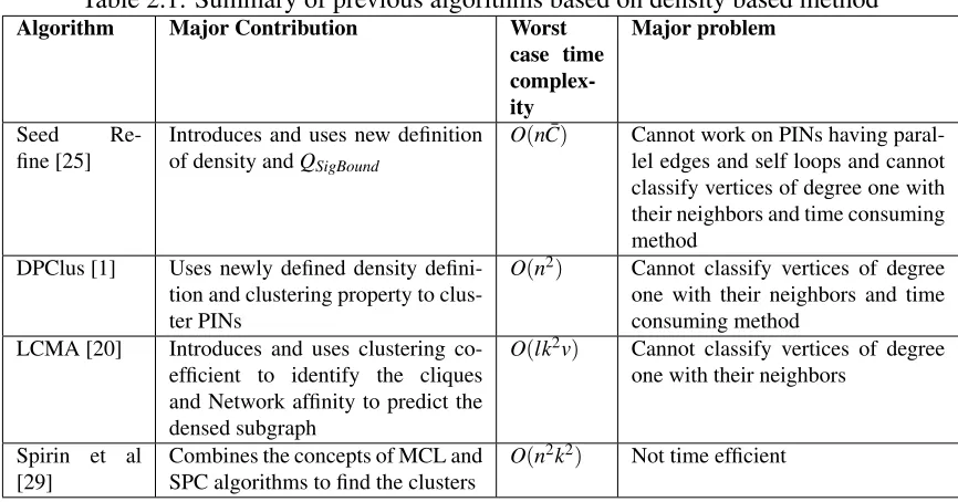
protein interaction networks in Table- 2.1. In the Table- 2.1, we have arrayed major

contri-bution, worst case time complexity and major shortcomings of each algorithms of density

based method.

Table 2.1: Summary of previous algorithms based on density based method

Algorithm Major Contribution Worst case time complex-ity Major problem Seed Re-fine [25]

Introduces and uses new definition of density andQSigBound

O(nC¯) Cannot work on PINs having

paral-lel edges and self loops and cannot classify vertices of degree one with their neighbors and time consuming method

DPClus [1] Uses newly defined density

defini-tion and clustering property to clus-ter PINs

O(n2) Cannot classify vertices of degree

one with their neighbors and time consuming method

LCMA [20] Introduces and uses clustering

co-efficient to identify the cliques and Network affinity to predict the densed subgraph

O(lk2v) Cannot classify vertices of degree one with their neighbors

Spirin et al

[29]

Combines the concepts of MCL and SPC algorithms to find the clusters

(34)

2.2 Graph partitioning approaches

In the current Section, we discuss the graph partitioning approaches to predict the

commu-nities in PINs. All partitioning algorithms detect the edges which are acted as the bridge

between communities. By removing bridge edges, the algorithms identify the clusters of

PINs.

2.2.1 Dongen 2000

S. V. Dongen designed an algorithm based on graph partition in his Ph.D. thesis. This

algorithm is known as Markov Cluateringalgorithm, in shortMCL. MCL algorithm was

designed based on random walk between the nodes of the graph. Random walk is calculated

by exponential normalized adjacency matrix and inflation parameter r. After calculating

random walk, MCL removes the edges with lower random walk values to separate the

clusters from network. This algorithm is commonly used in graph clustering. The worst

case time complexity of the MCL algorithm is O(n2p) where n and p are the number

of nodes in PINs and passes or random walk respectively. Its efficiency depends on the

selection of inflation parameterrand power parametere. Wrong selection ofrandemakes

the algorithm inefficient.

2.2.2 King et al. 2004

In the year 2004, a cost function based community detection algorithm was designed by

King et al [17] for predicting protein complexes. Their algorithm is known asRestricted

Neighborhood Search Clustering (RNSC)algorithm. This algorithm is devised on basically

(35)

edges) and assign a cost by using cost function which is not clearly mentioned in their

paper. After that, the algorithm separates the clusters from others by removing low cost

edges. RNSC gives good results for Giot et al [11]’s fruit fly’s protein interaction network.

Except this species, RNSC algorithm finds fewer complexes for all species. Besides, the

result of the algorithm heavily depends on the initial value which is random.

2.2.3 Graph Entropy Algorithm

Recently, Kenley et al [16] has designed a new graph partition algorithm based on graph

entropy. The graph entropy is defined based on the probability distribution of its inner links

and outer links. It is denoted ase(G).

e(G) =

_∑

vεV e(v) (2.6)

where

e(v) =−pi(v)log2pi(v)−po(v)log2po(v) (2.7)

Here po(v) and pi(v) denotes the probability of v having outer link and inter links

respectively. The graph entropy measure the cluster quality effectively. A graph with lower

entropy indicates that the vertices in the cluster have more inner links and less outer links.

The algorithm starts it working by selecting a random seed vertex and its neighbors

as seed cluster. After that, it iteratively adds or delete the vertices on the border of the

cluster to minimize the graph entropy. To produce a final set of cluster, the process of

seed selection and optimal cluster generation is repeatedly performed until no seed vertex

is remaining. This algorithm is known asGraph Entropyalgorithm. The time complexity

(36)

complexes and modules.

2.2.4 Summary

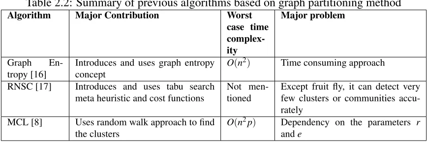
Here we have shown the summery of the graph partition based methods designed for

clus-tering protein interaction networks in Table- 2.2. In the Table- 2.2, we have arrayed major

contribution, worst case time complexity and major shortcomings of each algorithms of

graph partition based method.

Table 2.2: Summary of previous algorithms based on graph partitioning method

Algorithm Major Contribution Worst case time complex-ity Major problem Graph En-tropy [16]

Introduces and uses graph entropy concept

O(n2) Time consuming approach

RNSC [17] Introduces and uses tabu search

meta heuristic and cost functions

Not men-tioned

Except fruit fly, it can detect very few clusters or communities accu-rately

MCL [8] Uses random walk approach to find

the clusters

O(n2p) Dependency on the parameters r

ande

2.3 Hierarchical based methods

In this Section, we have discussed the previous hierarchical methods which are used to

identify the communities in PINs. Hierarchical methods use some measures to calculated

the similarity or compactness between nodes or communities for forming clusters. These

methods can be classified into two groups:agglomerativeanddivisive.

In agglomerative approach, at first all vertices are considered as individual clusters

which are known assingletons. After calculating similarity or compactness by using

(37)

value etc.), this approach merges two communities according to their most similarity or

compactness. This process continues until the graph remains one community.

Divisive approach is opposite of agglomerative approach. In this approach, a network is

considered as a community. After calculating similarity or compactness by using measure,

it divides the community into multiple communities according to their less similarity or

compactness. It continues until all vertices are represented as singletons.

2.3.1 Ravasz et al. 2002

Ravasz et al [27] proposed an agglomerative hierarchical clustering approach to identify the

protein complexes from PINs. Their algorithm has been designed on the basis of density

of the clusters. For identifying or calculating the density of the subgraph, they have used

Clustering Coefficient Valueswhich is as

followed-cc(G´) = 2×e

|k_i| ×(|k_i| −1) (2.8)

whereeis the number of edges connecting thekinearest neighbors of nodei. They are first

designers for introducing hierarchical methods for clustering protein interaction networks.

The time complexity of the algorithm isO(n2). The problem of this method- it cannot work

properly on scale free PINs. It takes more time to execute the algorithm for larger PINs

having more than hundred thousands proteins.

2.3.2 Girvan et al. 2002

Girvan and Newman proposed a new approach in hierarchical methods to classify PINs

(38)

this algorithm, Girvan and Newman introduced a new measure for clustering PINs. This

measure is known asedge betweenness. Theedge betweennessof an edge is the number of

shortest paths between pairs of nodes that run along it. If there is more than one shortest

path between a pair of nodes, each path is assigned equal weight such that the total weight

of all of the paths is equal to unity. If a network contains communities or groups that are

only loosely connected by a few intergroup edges, then all shortest paths between different

communities must go along one of these few edges. Thus, the edges connecting

commu-nities will have high edge betweenness (at least one of them). By removing these edges,

the groups are separated from one another and so the underlying community structure of

the network is revealed. This algorithm followsdivisiveapproach. The time complexity of

GN algorithm isO(m2n)wheremandnare the number of edges and vertices respectively.

GN algorithm is one of the most used algorithm in the field of bioinformatics. Though it is

most commonly used, GN algorithm has two major

shortcomings-• It is very time consuming algorithm. Generally, the number of edges in PINs are

larger than the number of vertices.

• It also faces the problem of clustering vertices of degree one.

2.3.3 Newman 2003

Newman designed a new hierarchical algorithm which is faster than GN algorithm. He

proposed his algorithm in his paper ”Fast algorithm for detecting community structure in

network” [22]. This agglomerative algorithm was designed on the basis ofmodularity, Q

-Q=

k

∑

i=1

(39)

where, wheree_iiis the fraction of edges with both end vertices in the same communityi,

anda_iis the fraction of edges with at least one end vertex in communityi. In agglomerative

steps, two communities are merged together if∆Qincreases or fixed. ∆Qfollows following

equation-∆Q=2(ei j−ai∗aj) (2.10)

The time complexity of the Newman’s algorithm is O((m+n)n) for PINs. Though

Newman’s algorithm is faster in comparison with GN algorithm, for PINs still it is time

consuming algorithm. On the other hand, for rat and mouse PINs, it suffers the second

problem of GN algorithm.

2.3.4 Radicchi et al 2004

Radicchi et al. [26] designed a new hierarchical algorithm based on the definition of weak

and strong communities. According to the definitions of weak and strong modules, they

introduced edge clustering coefficient in hierarchical algorithm to improve time

complex-ity. After calculating edge clustering value of each edge, their algorithm works like GN

algorithm but at every step, the removed edges are those with the smallest value of ˜C_i,_j.

˜

Ci,j=

Z_i,j(3)

min[(k_i−1),(k_j−1)] (2.11)

Here, C˜i,j is the modified edge clustering coefficient, Z_i,j(3) is the number of triangles

built on that edge (i,j) and min[k_i−1,k_j−1] is the maximal possible number of them.

The time complexity of the algorithm is O(m2). Though the algorithm is faster than GN

(40)

problem-if a community does not have any triangle or having a cycle, this algorithm is not efficient

enough [30].

2.3.5 Clauset et al 2004

Dr. Aaron Clauset and his supervisors Dr. M.E.J. Newman and Dr. C. Moore has designed

a new agglomerative hierarchical algorithm which used the concept of∆Q. Their algorithm

is the improved version of Newman’s ∆Qhierarchical algorithm [22]. For improving the

performance, they modified∆Q

-∆Qi,j=      1 2m−

di∗dj

(2m)2 ifiandiare connected

0 otherwise.

(2.12)

Wherediis the degree of vertexi. For improving time complexity, they usedmax heap

and sparse matrixto store the value of∆Q. Their proposed algorithm is known as CNM

algorithm. They algorithm works as

follows-• It calculates the initial values of∆Qi,j and store the largest value of each row of the

sparse matrix in max heap.

• It selects the largest∆Qi,j, merge two communitiesiand j.

• After merging, it recalculates the∆Qi,j and repeats the above step until one

commu-nity remains.

The time complexity of the algorithm is O(mhlog₂n)whereh is the depth of

dendro-gram. This algorithm improves the time complexity in significant amount. But it suffers

the common problem in hierarchical approach- clustering vertices of degree one in separate

(41)

2.3.6 Luo et al 2007

In 2007, a new agglomerative approach was introduced based onedge betweennessby Luo

et al [21]. Like GN algorithm, it calculates the edge-betweenness of all edges and sorted

them in ascending order. After that it

follows-• If the edge connects the vertices in same subgraph, it is added to the subgraph [21].

• If the edge connects the vertices in two different subgraph, two subgraphs are added

with satisfying one of two

conditions-– Two subgraphs are non-modules (non-module subgraph contains only one ver-tex).

– One subgraph is module and another one is non-module.

The process continues till|E|6=0. This algorithm is known asMoNetalgorithm. The

time complexity of MoNet algorithm is O(m2n). This algorithm also suffers same the

shortcomings as the GN algorithm.

2.3.7 Li et al. 2008

Min Li and her colleagues designed an agglomerative hierarchical algorithm based on edge

clustering value [19]. They have modified the formula of edge clustering coefficient. Their

modified edge clustering coefficient is as follows:

CC=|Ni∩Nj|+1

min(di,dj)

(2.13)

where, N_iandd_i are the neighbor list and degree of vertexirespectively. As per their

(42)

for all edges. After that, all singletons are merged together by the edges which are sorted in

descending order according to edge clustering coefficient values. The algorithm is known

as FAG-EC algorithm. The time complexity of the algorithm is O(d¯2m). Here ¯d is the

average degree of the network. The algorithm has one major problem. If in a PIN, a

good cluster has no triangle or has cycle, the edge clustering coefficient formula produces

low values for its (cluster’s inside) edges. For this reason, the FAG-EC algorithm cannot

produce accurate clusters.

2.3.8 Wang et al 2011

Min Li and her colleagues proposed a new algorithm based on the problem of their previous

algorithm FAG-EC which is known as HC-PIN algorithm [30]. In their algorithm, they

introduced a new measure to overcome the problem of FAG-EC algorithm. This measure

is calledEdge Clustering Value (ECV).

ECV = |Nu∩Nv|

2

|Nu| × |Nv|

(2.14)

WhereN_uis the set of neighbors of vertexv. They also redesignedECV for weighted

PINs which is as

follows-ECV∗= ∑kεIu,vw(u,k)×∑kεIu,vw(v,k) ∑sεNuw(u,s)×∑sεNuw(u,s)

(2.15)

where Iu,v denotes the set of common verticesNu and Nv. The Equation 2.14 is the

special case of Equation 2.15. Except the calculation of ECV, HC-PIN algorithm works

like FAG-EC algorithm. The time complexity of HC-PIN algorithm is O(d¯2m). Though

(43)

over weighted PINs, it suffers a common problem of hierarchical approach: classifying the

vertices of degree one in separate clusters from their neighbors.

2.3.9 Summary

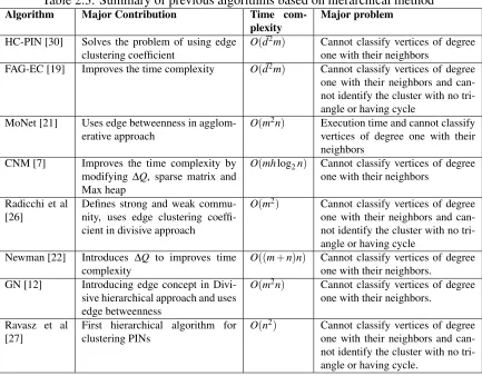
Here we have shown the summery of the hierarchical methods designed for clustering

pro-tein interaction networks in Table- 2.3. In the Table- 2.3, we have arrayed major

contribu-tion, worst case time complexity and major shortcomings of each algorithms of hierarchical

method.

Table 2.3: Summary of previous algorithms based on hierarchical method

Algorithm Major Contribution Time com-plexity

Major problem

HC-PIN [30] Solves the problem of using edge

clustering coefficient

O(d¯2m) Cannot classify vertices of degree

one with their neighbors

FAG-EC [19] Improves the time complexity O(d¯2m) Cannot classify vertices of degree

one with their neighbors and can-not identify the cluster with no tri-angle or having cycle

MoNet [21] Uses edge betweenness in

agglom-erative approach

O(m2n) Execution time and cannot classify

vertices of degree one with their neighbors

CNM [7] Improves the time complexity by

modifying ∆Q, sparse matrix and Max heap

O(mhlog₂n) Cannot classify vertices of degree one with their neighbors

Radicchi et al [26]

Defines strong and weak commu-nity, uses edge clustering coeffi-cient in divisive approach

O(m2) Cannot classify vertices of degree

one with their neighbors and can-not identify the cluster with no tri-angle or having cycle

Newman [22] Introduces ∆Q to improves time

complexity

O((m+n)n) Cannot classify vertices of degree one with their neighbors.

GN [12] Introducing edge concept in

Divi-sive hierarchical approach and uses edge betweenness

O(m2n) Cannot classify vertices of degree

one with their neighbors.

Ravasz et al [27]

First hierarchical algorithm for clustering PINs

O(n2) Cannot classify vertices of degree

(44)

(45)

Fast Agglomerative Clustering

Algorithms

We have discussed our proposed algorithm: FAC-PIN and premetric: relative

vertex-to-vertex clustering value in detail in this Chapter. Our designed FAC-PIN algorithm has

been developed based on the second, third and fourth properties of PINs. We have briefly

described the premetricrelative vertex-to-vertex clustering valuein Section 3.1 and

FAC-PIN algorithm with its computational complexity in Section 3.2.

3.1 Relative Vertex-to-Vertex Clustering Value

The edge clustering value,ECV(u,v), used in HC-PIN [30], is a similarity metric between

the two verticesuandvof an edge (u,v)and which, roughly speaking, tells how likelyu

andvlie in the same module (i.e., cluster). This is also true with the edge clustering

coeffi-cient,Cu,v(3), of [26]. However, in complex networks following the power law (i.e., scale-free

networks), it is reasonable to assume that the likelihood of a vertexuto lie in the same

(46)

ule asv(or, to lie in the module containingv), is not equal to the likelihood ofvto lie in the

module containingu. This assumption stems from the principle ofpreferential attachment

in scale-free networks which states that a new node uis likely to attachto a high-degree

nodevthan to a low degree node. This is not reciprocal, and hence, clearly suggesting that

the likelihood is not symmetric and that it is larger foruto be in a cluster withvthan forv

to be in cluster withu(if we assume thatvis a high-degree node). The similarity metrics

ECV(u,v)andCu,v(3)treat equally both endpoints of edges(u,v)irrespective of their degrees.

Also, another issue is that both ECV(u,v)andCu,v(3) require vertices uandv be connected

by an edge. This requirement is quite restrictive and we aim to extend to the case in which

pair (u,v) is not an edge while still being able to decide if both vertices are in the same

cluster. Finally, as stated earlier in previous section, current hierarchical approaches have

the common problem of classifying low-degree vertices (peripheral to dense subnetwork

modules) into separate clusters rather than merging them with their neighboring modules.

In the following paragraph, we present a new measure which aims to address these issues.

LetN_ube the set of neighbors of vertexuin an undirected graphG= (V,E). We define

N_u+=N_u∪ {u}as the neighbor set ofuaugmented withuitself. Given two verticesuand

v, we define the clustering value ofurelative tovas:

R(u_99Kv) = |N

+

u ∩Nv+|

|Nu+|

(3.1)

R(u_99Kv)is a premetric that ranges from 0 to 1; that is, it is a measure which does not

satisfy the axiom of symmetry and the triangle inequality but satisfies the axioms of

self-similarity and minimality. A vertexuwith a larger clustering value given another vertexv

is more likely to lie in the cluster containing v. In the followingC(a) denotes the cluster

(47)

of a community [26] (we use the term ws-cluster, hereafter). The following describe the

properties ofR(u_99Kv).

Given an edge(u,v),R(u_99Kv)is maximal (i.e. equals 1) if and only if|N_u+|=|N_u+∩

N_v+|. There are two cases achieving the maximum given edge(u,v):

1. whenuhas degree one

2. when bothuandvhave the same degree and|N_u+|=|N_v+|that is, they have the same

neighbors.

In either case, If sub-network C(v) (respectively, the induced sub-network of G for

subsetN_v+) is a ws-cluster then{u} ∪C(v)(respectively,{u} ∪N_v+) is a also a ws-cluster.

Given an edge (u,v), R(u_99Kv)is minimal when uis the highest degree vertex in G

andvhas degree 1; that is,R(u_99Kv) =₁₊_deg2₍_u,G₎ anddeg(u,G)is maximal. In such case,

R(v_99Ku) is maximal (i.e. equals 1), and hence,C(u)∪ {v}(respectively,N_u+∪ {v}) is a

ws-cluster ifC(u)(respectively,N_u+) is a ws-cluster. Here, we have found that R(v_99Ku)

solves the problem of clustering the vertices of degree one.

Given an edge(u,v), assume the degrees of verticesuandvinGare such thatdeg(u,G) =

deg(v,G) =dis maximal and thatuandvdo not share any other neighbors. Then, we have

R(u_99Kv) =R(v_99Ku) = ₁₊2_d ≤0.5 assumingd≥3. In this case,{u} ∪C(v)(orN_v+) is

not a ws-cluster, and,{v} ∪C(u)(orN_u+) is not a ws-cluster. Consider the induced subgraph

ofGonN_u+∪N_v+, we define thelocal betweenness valueof edge(u,v)as the percentage of

paths from vertices inN_u_rN_v to vertices inN_v_rN_ugoing through edge (u,v). Given the

number of common neighbors between uandv, |N_u∩N_v|, the local betweenness of edge

(u,v)is thus l(u,v) =100·_|_N 1

u∩Nv|+1. Given two connected high-degree vertices uand v,

(48)

it corresponds to when bothR(u_99Kv)andR(v_99Ku)values are small at the same time.

Edges with high local betweenness values are edges connecting two clusters, and therefore,

verticesuandvshould not lie in the same cluster.

Finally, our relative vertex clustering values implements the ideas behind the edge

clus-tering coefficient,Cu,v(k), of [26], since for a given vertex vand a neighboruthe number of

triangles given edge(u,v)is exactly|Nu∩Nv|; anduwill be included intoC(v)whenever

most of the neighbors ofu(excludingv) are inN_u∩N_v. This is also true even when(u,v)

is not an edge; in such case,|N_u∩N_v|relates to the number of squares containing vertices

uandv. On the other hand, we break through the limitations of [26] as in the edge

cluster-ing value,ECV(u,v) of [30], by not assuming the existence of closed loops in a network,

such as triangles or high-order loops. The relative vertex clustering value R(u_99Kv)also

improves ECV(u,v) since neighbors u of v which have most of their neighbors forming

a triangle with v are selected for inclusion inC(v). Searching for vertices uwhich form

a cluster withv is also more efficient than searching for edges (u,v)that makes a cluster

since the number of edges is larger than the number of vertices in dense subgraphs.

In summary, the values R(u_99Kv) and R(v_99Ku) for edge (u,v) can be used as a

quick test for deciding whetheru(respectively,v) should be merged with the clusterC(v)

(respectively,C(u)) such that{u} ∪C(v)(respectively,{v} ∪C(u)) remains a ws-cluster.

We have designedR(u_99Kv)based on the concept of preferential attachment property

of protein interaction networks. It calculates the likelihood value of any vertexv to form

cluster with another vertexu. On the other hand,Edge Clustering Value of Equation 2.14

was designed for each edge not for vertices. Our designedR(u_99Kv)is a premetric1. But

ECV of HC-PIN algorithm is similarity metric.

(49)

3.2 The FAC-PIN Algorithm

3.2.1 The algorithm

Our proposed fast agglomerative clustering algorithm for protein interaction networks,

FAC-PIN in Algorithm 1, goes as follows. Given a PIN G = (V,E), we initially

con-sider each vertex as a singleton, and sort the vertices v∈V in descending order of their

degrees deg(v,G) inG. Here we have used the second property of community structure.

After sorting, in an iterative manner, we select the next highest-degree vertex vfrom the

sorted list, and compute the valuesR(u_99Kv)andR(v_99Ku)for each neighboruofv, and

then decide depending on these two values and a thresholdα,0≤α≤1, whetherushould

be included inC(v)or not.

In the FAC-PIN algorithm, a neighboruof vertex vis added to the currentC(v)when

the majority of the neighbors ofuare inN_u+∩N_v+, that is when:

1. R(u_99Kv) =1, in which case eitheruhas degree 1, oruandvhave the same degree

and the same set of neighbors;

2. R(u_99Kv)>R(v_99Ku)>α, in which case uhave smaller degree thanvand most

of the neighbors ofuare in the intersection; and

3. R(u_99Kv) =R(v_99Ku)and the size of the intersection is larger than the total set of

neighbors ofuandvwhich are not in the intersection.

3.2.2 Computational Complexity

Letn=|V|be the number vertices,m=|E|be the number of edges, and ¯d be the average

(50)

Algorithm 1TheFAC-PIN Algorithm

Input:G= (V,E): undirected PIN graph α: threshold parameter

Output:P_k={C₁, . . . ,C_k}: identified collection of modules

{Initialization phase} foreveryv_i∈V do

C(v_i)← { {v_i},0/ };{each vertex is a singleton cluster}

end for

Sort all vertices to a priority-queueHin non-increasing order of their degrees;

{Community detection phase} repeat

v←H;{select next highest-degree vertex in H} forallu∈N_vnot yet merged into a clusterdo

if[R(u_99Kv) =1] Or [R(u_99Kv)>R(v_99Ku)>α]then C(v)←C(v)∪ { {u},{(u,v)} };

C(u)←C(v);

else

if [R(u_99Kv) =R(v_99Ku)] ≥α And [deg(u,G) +deg(v,G)−1 ≤ |Nu∩Nv|]

then

C(v)←C(v)∪ { {u},{(u,v)} };

C(u)←C(v);

end if end if end for untilH=0/ U ←V;

i←1;

{Compute the partitionP_k} whileU 6=0/ do

v←randomly select a vertex fromU;

C_i←C(v);

U ←U_r{u|C(u) =C(v)};

i←i+1;

end while

returnP_k← {C1, . . . ,Ck};

(51)

their degree isO(n)by using thecounting sortmethod, and the complexity of computing

the partition after the community detection phase is also O(n). Let the maximum node

degree inGbe d_max=maxv∈Vdeg(v,G). The complexity of computingR(u99Kv)given

verticesuandvin the ”for-loop” of FAC-PIN isO(dmax). The complexity of the ”for-loop”

is then O(d_max2 ), and hence, the total complexity of the ”repeat-loop” (and thus of

FAC-PIN) is O(nd_max2 )O(n3). Since PINs are power-law networks then the majority of the

proteins interact with only very few proteins, and thus the average degree ¯d is generally

small and can be considered a constant [30]; that is, we can use ¯d as the principal variable

for measuring the complexity of community detection methods. As such, then the worst

case time complexity of FAC-PIN isO(nd¯2)O(nd_max2 )O(n3). The worst case time

complexity of the HC-PIN algorithm of [30] isO(md¯2)and is larger than that of FAC-PIN

since n_≪min PINs. We note that HC-PIN is currently the fastest hierarchical method

(52)

(53)

Computation experiments, results and

discussions

We tested our FAC-PIN algorithm using several test procedures to understand its

work-ing capability on PINs. For experiment purpose we used protein interaction networks of

sixteen different species. We set the threshold parameter α in the FAC-PIN algorithm to

values 0.75, 0.5, 0.25, 0.125, 0.0625, 0.03125, 0.0156, 0.0078 and 0.0039 and ran

FAC-PIN with each of these values. After generating clusters of each protein interaction network

for eachα, a mathematical function is used to evaluate the clusters of a protein interaction

network. This mathematical function is known as scoring function. Scoring function

de-fines the compactness or density of a cluster. Most of the cases, higher scoring function

indicates clusters of the PIN are dense and loosely connected with rest of the clusters. In

the experiments, modularity Q[7, 22] andw- log -v[18] are used as scoring functions. In

this case, the clustered protein interaction network of highest scoring function is considered

as clustered PIN of a specific species. After clustering, clusters of PIN compared with the

physical complexes and identified functional modules of PIN of a species by using complex

(54)

Table 4.1: Dataset used in experiments

Species Scientific name Proteins Interactions Used symbol

Database

Baker’s yeast Saccharomyces cerevisiae 4572 49830 Y4K

2

5697 50675 Y5K 3

Cattle Bos taurus 5737 113888 C5K 3

Dog Canis lupus familiaris 2932 38647 D2K 3

E. coli Escherichia coli 2817 13841 E2K 1

Finch bird Taeniopygia Guttata 3929 74314 FB3K 3

Flowering plant (Thale cress)

Arabidopsis thaliana 2651 5236 FP2K 1

Fruit fly Drosophila melanogaster 8366 25611 FF8K 1

Frog Xenopus Tropicalis 5473 122706 FG5K 3

Jungle fowl (Chicken)

Gallus gallus 4960 112250 J4K 3

Human Homo sapiens 12994 135935 H12K

3

8997 34935 H8K 1

Mouse Mus musculus 2888 4372 M2K 1

Rat Rattus norvegicus 1148 1307 RA1K 1

Rice Oryza sativa 3778 320570 RI3K 3

Round worm Caenorhabditis elegans 4303 7747 RW4K 1

Wild boar Sus Scrofa 5303 119920 W5K 3

Zebra fish Danio rerio 8188 274358 Z8K 3

validation and functional module testing process respectively. we also compared the results

of FAC-PIN algorithm withHC-PIN andCNMalgorithms. Whole experiment process and

results are discussed in different sections of current Chapter.

4.1 Datasets

The PINs of sixteen different species were obtained from the PINALOG site1, the

Bi-oGRID database2 and REACTOME database3. The sixteen species are listed along with

their number of proteins and interactions in Table- 4.1.

From the Table- 4.1, it is found that the number of edges (interactions) is quite larger

than the number of vertices (proteins).

1

http://www.sbg.bio.ic.ac.uk/˜pinalog/downloads.html

2_{thebiogrid.org}

(55)

4.2 Testing by Scoring Functions

For given a clustering result (i.e. a partition)P_k={C1, . . . ,Ck}withkclusters, we used the

popular modularity functionQas one of the scoring function, introduced by Newman and

Girvan [7].

Q=

k

∑

i=1

(e_ii−a2_i), (4.1)

wheree_ii is the fraction of edges with both end vertices in the same communityi, and

a_i is the fraction of edges with at least one end vertex in communityi. kis the number of

clusters of the PIN. Larger values ofQcorrespond to more distinct community structures

in PINs. It means in-degree of a community i is larger than the out-degree of the same

communityi. ThoughQis widely used, it is known to have serious limitations which has

been discussed at length in [9]. The second partition scoring function we used has been

introduced in [18] and is defined as

w- log -v=

k

∑

i=1

(e_ii×loga_i). (4.2)

Function w- log -v allows for more diverse cluster sizes than function Q, It produces

negative values. Its smaller values corresponds to better clustered structures.

As said above, we ran FAC-PIN many times (each with different values of threshold

parameterα), then evaluate the clustered structure of the communities obtained by

FAC-PIN, and then retain the results giving the best scoring values. We also implemented the

best-performing HC-PIN algorithm of [30] and the hierarchical method of [7] which we

denote as the CNM algorithm. The HC-PIN and CNM methods were run on the same PIN

(56)

(CNM has no parameters). The results of the three methods are given in Tables 4.2, 4.3,

4.4, 4.5, 4.6 and 4.7, respectively in terms of scoring valuesQ andw- log -v, and running

times obtained by each method for each species. As well as we have showed the histogram

of modularityQ, w- log -vand log-log plot of time comparison of FAC-PIN, HC-PIN and

CNMalgorithms in Figures- 4.1, 4.2, 4.3, 4.4, 4.5 and 4.6 respectively.

Table 4.2: Qresults ofFAC-PIN,CNMandHC-PINfor Baker’s yeast, Cattle, Dog, E.coli, Finch bird, Flowering plant, Fruit fly and Frog.

Algorithms Y4K Y5K C5K D2K E2K FB3K FP2K FF8K FG5K

FAC-PIN 0.5415 0.5110 0.7288 0.7566 0.1492 0.7874 0.9422 0.6486 0.7432 CNM 0.5391 0.1412 0.6969 0.6850 0.0587 0.7199 0.7861 0.3116 0.6909 HC-PIN 0.5401 0.0387 0.5265 0.6405 0.0023 0.6075 0.7819 0.0086 0.4907

Table 4.3: Qresults ofFAC-PIN,CNMandHC-PIN for Human, Jungle fowl, Mouse, Rat, Rice, Round worm, Wild boar and Zebra fish.

Algorithms H8K H12K J4K M2K RA1K RI3K RW4K W5K Z8K

FAC-PIN 0.5893 0.7827 0.7540 0.7644 0.7897 0.5401 0.7484 0.7536 0.7692 CNM 0.4768 0.2858 0.7000 0.4781 0.5457 0.5215 0.4057 0.7040 0.2294 HC-PIN 0.2768 0.0126 0.6527 0.5015 0.4502 0.1791 0.2928 0.5180 0.7527

Table 4.4: −(w- log -)v results ofFAC-PIN, CNM and HC-PIN for Baker’s yeast, Cattle, Dog, E.coli, Finch bird, Flowering plant, Fruit fly and Frog.

Algorithms Y4K Y5K C5K D2K E2K FB3K FP2K FF8K FG5K

FAC-PIN 1.301 0.521 1.141 1.630 0.262 1.359 3.603 1.517 1.208 CNM 1.299 0.481 0.7173 1.278 0.192 1.119 2.866 1.233 0.997 HC-PIN 1.299 0.028 0.3162 0.998 0.019 0.847 3.071 0.072 0.516

Table 4.5: −(w- log -v) results ofFAC-PIN, CNM and HC-PIN for Human, Jungle fowl, Mouse, Rat, Rice, Round worm, Wild boar and Zebra fish.

Algorithms H8K H12K J4K M2K RA1K RI3K RW4K W5K Z8K

FAC-PIN 1.366 1.941 1.568 2.634 2.525 1.615 2.094 1.048 0.773 CNM 1.197 1.269 1.488 1.530 1.699 1.585 1.819 1.283 0.756 HC-PIN 0.566 0.113 1.283 1.805 1.558 0.237 1.809 0.760 0.262

As we see in both Tables 4.2, 4.3, 4.4 and 4.5, FAC-PIN outperformed both the HC-PIN

(57)

Y₄_K Y₅_K C5K D2K E2K FB3K FP2K FF8K FG5K

0 0.1 0.2 0.3 0.4 0.5 0.6 0.7 0.8 0.9 1

Modularity

,

Q

FAC-PIN CNM HC-PIN

Figure 4.1: Modularity comparison among FAC-PIN, CNM and HC-PIN algorithms for Baker’s yeast, Cattle, Dog, E.coli, Finch bird, Flowering plant, Fruit fly and Frog

H8K H12K J4K M2K RA1K RI3K RW4K W5K Z8K

0 0.1 0.2 0.3 0.4 0.5 0.6 0.7 0.8

Modularity

,

Q

FAC-PIN CNM HC-PIN

(58)

0 0.5 1 1.5 2 2.5 3 3.5

-( w -log -v )

FAC-PIN CNM HC-PIN

Figure 4.3: -(w- log -v) comparison among FAC-PIN, CNM and HC-PIN algorithms for Baker’s yeast, Cattle, Dog, E.coli, Finch bird, Flowering plant, Fruit fly and Frog

H8K H12K J4K M2K RA1K RI3K RW4K W5K Z8K

0 0.5 1 1.5 2 2.5

-( w -log -v )

FAC-PIN CNM HC-PIN

(59)

0 0.25 0.5 0.75 1 1.25 1.5 1.75 2 2.25 2.5 2.75 3 3.25

log(T

ime(Seconds))

FAC-PIN CNM HC-PIN

(60)

H₈_K H₁₂_K J₄_K M₂_K RA₁_K RI₃_K RW₄_K W₅_K Z₈_K