ABSTRACT
CHEN, JIANFENG. On the Value of Sampling and Pruning for Search-Based Software Engineering. (Under the direction of Timothy Menzies).
Software Engineering researchers use search-based software engineering (SBSE) optimization techniques to solve SE configuration problems with single or multiple objectives; e.g. (1) selecting partial features to develop to stratify the shareholders or (2) reducing development cost, or (3) minimizing testing suites while improving coverage, etc.
Most previous researchers in this area applied evolutionary algorithms or their variants,EVOL for short in this research, to those tasks. Due to the complexity of SE models, their algorithms are excessively CPU intensive.
This research explores an alternative approach –OSAP, short for over-sampling-and-pruning. OSAPperforms the oversampling and prunes the configurations, without evaluating all candidates. OSAPhas four generations, namedOSAP1,OSAP2, and so on.
The first generation ofOSAP,OSAP1, a.k.a. SWAY, assumed that a small region in decision space can lead to best objectives. Therefore, it separated the decision space by some specific separation metrics to prune poor regions. When applied to two widely-explored SE requirement engineering models – XOMO and POM3, SWAY generated new state-of-the-art results. SWAY also returned comparable configurations to another baseline method, which just selects the best set from large amount of randomly generated configurations.
Some models may not hold that assumption of the SWAY, such as the software product line (SPL) or next release planning (NRP). The SPL/NRP optimization requires to find the best set of features (to develop) under some constraints. The second generation ofOSAP,OSAP2, a.k.a. SWAY2, first divides the configurations into several groups, and then applies the SWAY in each group.
While successful in many domains, SWAY was proved to fail for more complex problems. For example, cloud computer configuration problems defeat SWAY since their best configurations do not gather in some regions in decision space. Based on an analysis of those failures, this research developed a novel variant, theOSAP3, or RIOT, that builds up a linear surrogate model to evaluate sampling and therefore leads to a faster pruning. On experimentation, RIOT outperforms not only SWAY but also methods proposed by numerous other researchers for cloud computing configuration.
study revisited the XOMO/POM3 models and the second study was the test suite generations for symbolic models (expressed as 3-SAT CNF). Experiments showed that the WORTHY outperformed theOSAP1, or had better results than state-of-the-art techniques.
© Copyright 2019 by Jianfeng Chen
On the Value of Sampling and Pruning for Search-Based Software Engineering
by Jianfeng Chen
A dissertation submitted to the Graduate Faculty of North Carolina State University
in partial fulfillment of the requirements for the Degree of
Doctor of Philosophy
Computer Science
Raleigh, North Carolina
2019
APPROVED BY:
Min Chi Emerson Murphy-Hill
Xipeng Shen Timothy Menzies
DEDICATION
To my parents.
BIOGRAPHY
Jianfeng Chen was born in Dongguan City, Guangdong Province in 1992. In 2014, he obtained his a B.Eng. Degree in Software Engineering from Shandong University China, where he worked closely with Dr. Yijun Yang in Research Center of Human-Computer Interaction & Virtual Reality. He started his PhD program from August 2014 in department of computer science, North Carolina State University. He joined Dr. Tim Menzies’s lab in 2015. During his PhD, he had an internship in Facebook (2018, Cambridge MA) and successfully participated in the Google Summer of Code program (2016), in the team of Java Pathfinder (JPF). He also had cooperation experiences with the Laboratory for Analytic Sciences (NCSU) as well as LexisNexis Legal & Professional (LNG-RDU).
ACKNOWLEDGEMENTS
Throughout my journey of my PhD program, I have received a great deal of support and assistant – this isnotan individual work.
I would first like to think my advisor, Dr. Tim Menzies, whose expertise was invaluable in pointing out my research directions in particular. Dr. Tim Menzies is a nice and experienced academic advisor. He could always give me some pressure in a correct time and in the suitable way, although sometimes his words contained some metaphors. I especially appreciated Dr. Menzies’s efforts in preparing my Oral Prelim Exam. At that time, he spent a lot of time in revising my lecture as well as the slides. Through that exam, my presentation skill was significantly improved. (Apparently, of course,) I still need to strengthen my communication skills. As the last point, I would like to say thank you for Dr. Menzies’s research fundings, which came from the NSF, LAS or LexisNexis etc. I am also grateful to my PhD committee members, Dr. Min Chi, Dr. Emerson Murphy-Hill and Dr. Xipeng Shen, for all the time spent, all the help and advice on my research and career.
I would like to thank every (current or former) members in RAISE lab. They are Dr. Wei Fu, Dr. Vivek Nair, Di Chen, Rahul Krishna, George Mathew, Zhe Yu, Amrit Agrawal, Patrick Xia, Huy Tu, Rui Shu, Xueqi Yang, Shrikanth NC, Joy Chakraborty, Fahmid Fahid and Dr. Junjie Wang, our distinguished visiting scholar from Chinese Academy of Science. I had very insightful discussions with Dr. Vivek Nair, Zhe Yu etc. Rahul and George answered many of my silly programming questions. Patrick saved me a lot of money in travelling and entertainments... Some of them were also my coauthors – Vivek, Rahul, Patrick, Junjie, et al. We worked and shared our opinions around the Room 3240 at EBII. Every one in the lab helped me a lot in different ways. So thank you all very much!
I am grateful to my new friends in NC State University. Here is a partial list of them: Shengpei Zhang, Rui Zhi, Wengran Wang, Hao Pang, Zexi Chen, Boxuan Zhong, Rong Huang, Jerry Lee, Bowen Li, Gina R. Bai, Weijie Zhou, Justin Smith, Zhewei Hu, Shuai Yang, Pei Deng, Xin Pan, Chin-Jung Hsu, Answesha Das, Lingnan Gao, Akond Rahman, Ye Mao, Yiqiao Xu, Linting Xue, and so on. Thanks for all kinds of helps or supports in life or academic.
I also want to thank the partners during my intern or co-op programs. They are Neha Rungta – principal engineering at Amazon AWS, Aaron Roth – former Facebook engineer, Vlad Bychkovsky and Jenny Ramseyer – Facebook researchers, Philip Clark and Kevin Haverlock – LexisNexis engineers, Bojan Cukic – Chair of CS department in UNCC, etc. They brought me the insights from industrial world. In the meanwhile, I miss the friendship with colleagues during my Facebook Intern. They are Yi-Hsiu Chen, Allison Tielking, Macros Banchik, Stephanie Angulo, Anthony Simpson, Karen Guo, etc. Thanks all for shring the funs in summer 2018.
I extend heartfelt thanks to the distinguished faculties and staffs at the department of computer science, including George Rouskas, Kathy Luca, Carol Allen, Todd Gardner, etc. Thanks for the helps
in these years!
Here I am grateful to Dr. Yijun Yang, a professor in School of Computing, Shandong University. He advised me a lot during my undergraduate. Thanks for encouraging me to apply for the PhD in North American.
Finally, last but not least, I am very thankful to my family and friends, who have been beside me, supporting me and helping me at all times.
TABLE OF CONTENTS
LIST OF TABLES . . . ix
LIST OF FIGURES. . . x
Chapter 1 Introduction. . . 1
1.1 Statement of Thesis . . . 2
1.2 Generations of OSAP . . . 3
1.2.1 First Generation of OSAP, a.k.a. SWAY . . . 3
1.2.2 Second Generation of OSAP, a.k.a. SWAY2. . . . 3
1.2.3 Third Generation of OSAP, a.k.a. RIOT . . . 3
1.2.4 Fourth Generation of OSAP, a.k.a. WORTHY . . . 5
1.3 Study Cases Overview . . . 5
1.3.1 XOMO and POM3 . . . 5
1.3.2 Software Product Line (SPL) . . . 5
1.3.3 Next Release Problem (NRP) . . . 6
1.3.4 Workflow Deployment in Cloud Environment . . . 6
1.3.5 Test Suite Generation . . . 6
1.4 Publications from this Thesis . . . 6
1.5 Structure of this Dissertation . . . 7
Chapter 2 Why SBSE Need Faster, Simpler Methods. . . 8
2.1 What is the Value of Seeking Simplicity? . . . 8
2.2 Why not just Use More of the Cloud? . . . 9
2.3 OSAP as a Baseline Optimizer . . . 9
2.3.1 Why Researchers Need Baseline Algorithm . . . 9
2.3.2 Principles for Baseline Algorithms in SBSE . . . 10
2.3.3 Can OSAP be a Baseline Optimizer? . . . 10
Chapter 3 Problem Formulation. . . 12
3.1 Software Configuration Optimization . . . 12
3.2 Search Based Software Engineering . . . 13
3.3 Measuring the Efficiency . . . 14
3.4 Measuring the Effectiveness . . . 14
3.4.1 Effectiveness Measuring in Single-objective Problem . . . 14
3.4.2 Standard Metrics for Multi-objective Problems . . . 14
3.4.3 Problem-Specified Measurements . . . 16
3.5 Choice of Statistical Ranking Methods . . . 16
Chapter 4 Over-Sampling-and-Pruning . . . 17
4.1 Evolutionary Algorithms . . . 17
4.2 Over-sampling and Pruning . . . 20
4.3 EVOL versus OSAP . . . 20
Chapter 5 SWAY, First Generation of OSAP . . . 22
5.1 Implementations of SWAY . . . 23
5.2 Case Study: XOMO and POM3 . . . 24
5.2.1 Benchmarks of XOMO . . . 28
5.2.2 Benchmarks of POM3, a Model of Agile Development . . . 29
5.2.3 Experiment Design . . . 31
5.2.4 Is SWAY Faster than Typical EVOL? . . . 32
5.2.5 Are SWAY’s Solutions as good as Other Optimizers? . . . 33
5.2.6 Threats to Validity . . . 36
5.3 Summary of OSAP1 . . . 37
Chapter 6 SWAY2, Second Generation of OSAP . . . 38
6.1 When is OSAP1 most Useful, Useless? . . . 38
6.2 Initial Splitting with Expert Knowledge . . . 39
6.3 Case Study I: Software Product Line optimization . . . 40
6.3.1 An implementation of SWAY2, Splitting the Discrete Space . . . 40
6.3.2 Software Product Line Optimizations . . . 42
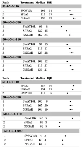
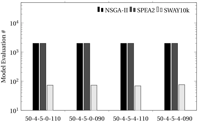
6.3.3 Result I: Comparing the Efficiency . . . 46
6.3.4 Result II: Comparing the Effectiveness . . . 46
6.4 Case Study II: Next Release Problem . . . 47
6.4.1 Split Function for Discrete Models (NRP) . . . 47
6.4.2 The NRP problem . . . 47
6.4.3 Case Study Research Questions . . . 49
6.4.4 Experimental Setup . . . 49
6.4.5 Results . . . 50
6.5 Comments on the Simplicity of SWAY . . . 52
6.6 Summary of OSAP2 . . . 54
Chapter 7 RIOT, Third Generation of OSAP . . . 55
7.1 Linear Surrogate Model as the Selector . . . 55
7.2 Case Study: Workflow Deployment Optimizations . . . 57
7.2.1 Motivation . . . 57
7.2.2 Problem Formulation . . . 58
7.2.3 Related Work . . . 60
7.2.4 How to Make a RIOT (Methodology) . . . 62
7.2.5 Evaluations . . . 64
7.2.6 Threats to Validity . . . 67
7.3 Summary of OSAP3 . . . 68
Chapter 8 WORTHY, Fourth Generation of OSAP. . . 69
8.1 Delta Oriented Surrogate Model . . . 69
8.2 Case Study I: Revisit XOMO&POM3 . . . 71
8.2.1 Can the KNN Model Successfully Get the Sign of∆O i? . . . 71
8.2.2 Comparing Effectiveness on OSAP1 and OSAP4 . . . 72
8.2.3 Comparing the Efficiency . . . 79
8.3 Case Study II: Test Suite Generation . . . 79
8.3.1 Problem Formulation . . . 79
8.3.2 Related Work . . . 80
8.3.3 Motivation of this Work . . . 82
8.3.4 ApplyOSAP4to Test Suite Generation . . . 83
8.3.5 Experiment Design . . . 84
8.3.6 Are the Deltas Transferable? . . . 85
8.3.7 Can WORTHY Find Test Suite with Enough Diverse Faster? . . . 87
8.3.8 Can WORTHY Reduce the Size of Test Suite? . . . 88
8.3.9 Threats to Validity . . . 90
8.4 Summary of OSAP4 . . . 92
Chapter 9 Conclusions and Future Work. . . 93
9.1 Executive Summary . . . 93
9.2 Generations ofOSAPRevisited . . . 93
9.3 Study Cases Revisited . . . 94
9.4 Other Works Related to this Research . . . 95
9.4.1 Better Evolutionary Algorithms for SBSE . . . 95
9.4.2 Faster Evolutionary Algorithms . . . 96
9.4.3 Solving Problems via Sampling . . . 97
9.5 Future Work . . . 97
9.5.1 Ensemble Learning . . . 97
9.5.2 Better Exploring the Constrained Model . . . 98
9.5.3 Increasing Sampling for Modified Models . . . 98
BIBLIOGRAPHY . . . 99
LIST OF TABLES
Table 5.1 Parameters tuned by grid search for the NSGA-II. . . 32
Table 5.2 Parameter configurations overview . . . 32
Table 5.3 Median value of runtime and model evaluation numbers. . . 33
Table 5.4 Median value of runtime and model evaluation numbers. . . 36
Table 6.1 Feature models used in case study SPL. . . 46
Table 6.2 Median value of runtime and model evaluation numbers. . . 46
Table 7.1 Highly Cited Workflow Configuration Techniques from 2006 to present . . . 61
Table 7.2 Eight types of AWS EC2 instances. . . 64
Table 7.3 Median Runtime* among 30 Repeats in RIOT and Others . . . 65
Table 7.4 Median Measurements for all Experimented Workflows . . . 66
Table 8.1 Related work for solving theory proving constraints via sampling over recent decades. . . 81
Table 8.2 Benchmarks overview. Benchmarks are sorted by number of variables. . . 86
Table 8.3 Number of unique cases in the test suite. Benchmarks are sorted by number of variables. . . 91
LIST OF FIGURES
Figure 3.1 Schematic diagram of frontier quality measures. . . 15
Figure 4.1 Basic framework ofEVOL . . . 18
Figure 4.2 Basic framework ofOSAP . . . 20
Figure 5.1 Descriptions of the XOMO variables. . . 26
Figure 5.2 Four project-specific XOMO case studies. . . 27
Figure 5.3 List of inputs to POM3. . . 29
Figure 5.4 Three specific POM3 scenarios. . . 29
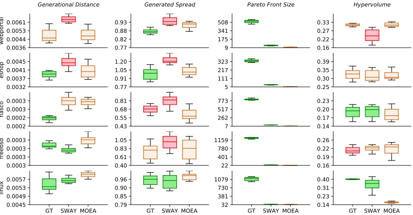
Figure 5.5 The box-plot of four quality indicators in each study cases . . . 34
Figure 5.6 GroundTruth vs state-of-the-art. . . 35
Figure 5.7 SWAY vs. state-of-the-art. . . 35
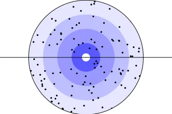
Figure 6.1 Map candidates into a circle by domain knowledge . . . 40
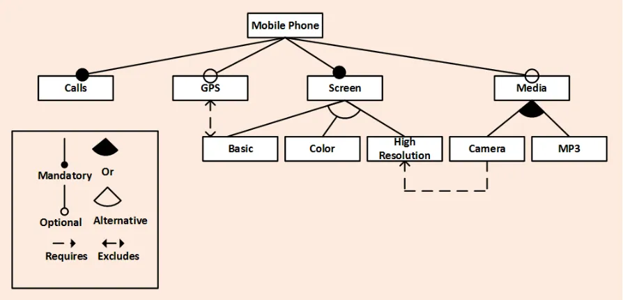
Figure 6.2 Feature model for mobile phone product line. . . 44
Figure 6.3 The box-plot of four quality indicators in each study cases (SPL) . . . 45
Figure 6.4 Variants of NRP used in this study. . . 48
Figure 6.5 Spread and hypervolumes seen in 20 repeats for NRP models. Upper: Spread (lessisbetter). Bottom: Hypervolume (moreisbetter). . . 51
Figure 6.6 Medium number of model evaluations for NRP models. . . 52
Figure 6.7 Seed the initial population of the traditional EVOL by SWAY. . . 53
Figure 7.1 RIOT surrogate model illustration. . . 56
Figure 7.2 Examples of cloud computing workflows. . . 57
Figure 7.3 A scheduling example that uniquely set the scheduling. . . 59
Figure 7.4 Framework of Standard Multi-objective Evolutionary Algorithms. . . 60
Figure 7.5 Demostration to group instances. . . 63
Figure 8.1 Predict∆O(y axis) vs. actual∆O(x axis) in XOMO models. . . 73
Figure 8.2 Predict∆O(y axis) vs. actual∆O(x axis) in POM3 models. . . 74
Figure 8.3 Comparisons on effectiveness SWAY and WORTHY for the XOMO models. . . 75
Figure 8.4 Comparisons on effectiveness on SWAY and WORTHY for the POM3 models. 76 Figure 8.5 Average runtime and number of model evaluations over 20 repeats for the XOMO models. . . 77
Figure 8.6 Average runtime and number of model evaluations over 20 repeats for the POM3 models. . . 78
Figure 8.7 A simple C++code script calculating the medium of three integers.[SK12] . . 79
Figure 8.8 Script of a CNF benchmark(LoginService2.sk_23_36) . . . 80
Figure 8.9 A demonstration ofZ3 fixing procedure. . . 84
Figure 8.10 Number of identical deltas among 100*100 pair of valid solution deltas for all benchmarks. . . 87
Figure 8.11 Normalized compression distance (NCD) got when the experiment terminated. 89 Figure 8.12 Sampling time required before execution got terminated. . . 90
CHAPTER
1
INTRODUCTION
Software engineers often need to answer questions that explore trade-offs between competing goals. This is particularly true when stakeholders propose multiple goals or requirements and software developers need to find good choices that most reflect and balance rival objectives such as:
1. What smallest set of test cases that cover all program branches?
2. What is the set of requirements that balances software development cost and customer satis-faction?
3. What cheapest resources achieve most functionality?
4. What sequence of refactoring steps take least effort while most decreasing the future mainte-nance costs of a system?
As modern software grows increasingly complex, it becomes difficult (or impossible) to manually find these good choices. Hence, in recent years, there has been an increasing interest in search-based software engineering, or SBSE (details see §3.2). SBSE often uses multi-objective evolutionary algo-rithms (EVOL)[Har12; Say13a]that explore generations of mutations to a population of candidate solutions. Examples of this kind of analysis include:
• Project planning: Ferrucci et al.[Fer13]modified the crossover operator in the NSGA-II algo-rithm and found that their approach (called NSGA-IIv) was useful for planning how to make
best use of project overtime.
• Test suite minimization: Wang et al.[Wan13a]showed that their “weighted-based” genetic algorithm significantly outperformed other methods using industrial case study for Cisco Systems.
• Improving defect prediction: Tantithamthavorn et at.[Tan16]report that software quality predictors learned from data miners can be improved if an evolutionary algorithm first adjusts the tuning parameters of the learner.
• Software clone detectors: Wang, Harman et al.[Wan13b]report that the arduous task of configur-ing complex analysis tools like software clone detectors can be automated via multi-objective evolutionary algorithms.
A drawback with standardEVOLis that they can be very computational expensive (see §4.1). This can make them problematic to apply, especially for complex problems. For example, in the above list, the last two studies required 22 days and 15 years of CPU time respectively.
One way to address this CPU cost is to use cloud-based CPU farms. The advantage of this approach is that it is simple to implement (just buy the cloud-based CPU time). But cloud-based resources have some disadvantages: (a) cloud computing environments are extensively monetized so the total financial cost of tuning can be prohibitive; (b) that CPU time is wasted time if there is a faster and more effective way.
This research explores a faster and more effective way to solve problems traditionally addressed byEVOL. Our new approach offers a novel prospective on SBSE research. It isnotsupposed to explorespecificalgorithms or techniques for some SE model.Instead, it explores the decision space (the space formed by all possible configurations in a SE problem)and the objective space(space of the corresponding objectives)in general software engineering models. This new method is called a over-sampling-and-pruning methods, or OSAP for short.OSAPassumes that by (a) generating many candidates; but (b) only evaluating a few of them, it is possible to retrieve good configurations for the SBSE model in a very short time. this research explores four generations in total.
1.1
Statement of Thesis
For the optimization of search based software engineering problems:
• Given a proper configurations selector or comparator, built upon decision space,
• Over-sampling and pruning is better than a standard mutation based evolutionary approach;
1.2
Generations of OSAP
This research developed four generations ofOSAP, labelled asOSAP1,OSAP2,OSAP3,OSAP4in current dissertation.
1.2.1 First Generation of OSAP, a.k.a. SWAY
OSAP1is the initial version ofOSAP. The configuration selector ofOSAP1is based on a simple (but maybe rough) assumption: the best configuration for a software engineering problem only appears in a small region of the decision space. Imposing this assumption, theOSAP1further develops a (decision) separator that bi-clusters the configurations.OSAP1pruned one cluster among them based on the evaluations of two representatives, one in each cluster. The pruning process is performed recursively under a small region is found. The method is also named as SWAY in the published paper.
1.2.2 Second Generation of OSAP, a.k.a. SWAY2
OSAP2is an improved version to OSAP1. It first requires the expert knowledge to divided the decision space. For example, in the requirement engineering problems, such division can be the size/scale of proposed configuration, measured by the number of features to be developed, etc. After dividing the decision space from expert knowledge, the SWAY is executed in each sub decision space. The optimal/desired configuration is the union set in each sub decision space. TheOSAP2 is also named as SWAY2in the publications.
1.2.3 Third Generation of OSAP, a.k.a. RIOT
OSAP
O
UTLINESOSAP1(SWAY)
-What was achieved:SWAY first found that sampling-and-pruning method can get similar results to mutation based evolutionary algorithm, in a much faster way.
-What was learned:The evolution inEVOLmay not be helpful. Given appropriate pruner, a small region in decision space could contain the optimal configurations.
-Limiting assumptions:Only valid for simple models which have the “golden” (decision space) region.
OSAP2(SWAY2)
-What was achieved:FixedOSAP1via doing the decision space partition first, using the domain /expert knowledge.
-What was learned:Utilizing the domain/expert knowledge could be helpful.
-Limiting assumptions:domain/expert knowledge is required; not flexible enough. To some extent, the “golden” region assumption still exists.
OSAP3(RIOT)
-What was achieved:Created a surrogate model that directly estimate the objectives of the configurations, leading to effective sampling and pruning.
-What was learned:Building a surrogate model to abridge the decision space and objective space is possible. Such surrogate model could be used as an alternative to replace the complex SE model.
-Limiting assumptions:The surrogate model was based on the linearity of the model.
OSAP4(WORTHY)
-What was achieved:Created another more flexible surrogate model without the dependence of linearity of the model.
-What was learned:Decision+configuration∆oriented surrogate models better explore more complex SE models.
1.2.4 Fourth Generation of OSAP, a.k.a. WORTHY
The effectiveness ofOSAP3is highly depending on the the “linear” interpolation surrogate models. To remove the “linearity” assumption,OSAP4directed built up the a surrogate model learning the decision spaceδ-vector of every pair of some evaluated configurations. Thek-nearest neigh-bor(KNN) can be used as the surrogate model. TheOSAP4is also named as WORTHY in the papers.
1.3
Study Cases Overview
The motivation for this work is not to solve a particular case study; instead, it explores an alternative framework to the slow evolutionary algorithms(EVOL). Therefore,OSAPshould be tested in diverse software engineering problems. By saying the “diverse”, it meant the following perspective:
• Problems appears from different stages in software development process;
• Covering the problems with no constraints, slight constraints, and highly constraints;
• The decision space has various types, such as numeric, enumerations, discrete, binary etc.
It is impossible to explore all search-based software engineering problems in a single research. The following study cases were explored and discussed in this dissertation.
Note: Statements on how the following study cases meets the diversity perspectives will be given at the end of this dissertation (§9.3).
1.3.1 XOMO and POM3
XOMO, introduced by Menzies et al.[MR05], is a general framework for Monte Carlo simulations that combines four COCOMO-like software process models from Boehm’s group at the University of Southern California.
POM3 model is a tool for exploring the thorny management challenge in agile development[BT03b; Por08; BT03a]– balancingidle rates,completion ratesandoverall cost.
1.3.2 Software Product Line (SPL)
1.3.3 Next Release Problem (NRP)
An other study case is the next release problem (NRP) come across in requirement engineering. NRP concerns with defining which requirements should be implemented for the next version of the systems, according to customer satisfaction, budget constraints as well as precedence con-straints between various requirements. Durillo et al.[Dur09], treated the next release problem as a multi-objective problem, since higher customer satisfaction and less development time or cost are conflicting objectives, we call this formulation as multi-objective NRP (MONRP). MONRP in this paper considers (maximizing) combination of importance and risk, (minimizing) cost and (maximizing) satisfaction.
1.3.4 Workflow Deployment in Cloud Environment
Scientific workflows (a.k.a data-intensive workflow) have been widely applied in scientific research, data mining and business intelligence analysis [Vöc11]. One fundamental problem in workflow research isworkflow scheduling, i.e. associating the appropriate computer resource to each task in the workflow.
1.3.5 Test Suite Generation
Theory proving is one of basic techniques in software testing. Given a program, modern symbolic execution[Bal18]and/or dynamic symbolic execution techniques[Chr16]are able to generate the constrained SAT models, expressed as CNF (conjunctive normal form) or DIMACS[BB17]form. Each valid solution is corresponding to a unique feasible test case in a program. Consequently, searching for solutions to the constraint model constructs a test suite to the corresponding program.
1.4
Publications from this Thesis
Conferences
• [Under Review]Jianfeng Chenand Tim Menzies. "On the Benefits of Restrained Mutation: Faster Generation of Smaller Test Suites" Submitted to IEEE/ACM International Conference on Automated Software Engineering (ASE 2019).
• [CM18]Jianfeng Chen, and Tim Menzies. "RIOT: A Stochastic-Based Method for Workflow Scheduling in the Cloud." 2018 IEEE 11th International Conference on Cloud Computing (CLOUD). IEEE, 2018.
• [Nai16]Vivek Nair, Tim Menzies, andJianfeng Chen. "An (accidental) exploration of alter-natives to evolutionary algorithms for sbse." In International Symposium on Search Based Software Engineering, pp. 96-111. Springer, Cham, 2016.
Journals
• [Che18]Jianfeng Chen, Vivek Nair, Rahul Krishna, and Tim Menzies. "" Sampling" as a Baseline Optimizer for Search-based Software Engineering." IEEE Transactions on Software Engineer-ing (2018).
• [Xia18](Minor revision) Tianpei Xia, Rahul Krishna,Jianfeng Chen, George Mathew, Xipeng Shen, and Tim Menzies. "Hyperparameter optimization for effort estimation." Empirical Software Engineering (EMSE), 2018
• [Che17]Jianfeng Chen, Vivek Nair, and Tim Menzies. "Beyond evolutionary algorithms for search-based software engineering." Information and Software Technology (2017).
1.5
Structure of this Dissertation
The rest of this dissertation is structured as follows.
• Chapter 2 motives the whole research, answering a frequently asked question – “why we need to replace theEVOL?”
• Chapter 3 formulates the search-based software engineering, including problem definition, evaluations of solvers and statistical ranking for various solvers.
• Chapter 4 is the overview of two strategies in solving SBSE: evolutionary algorithm and over-sampling-and-pruning.
• Chapter 5 to Chapter 8 introduce four generations ofOSAP. Each of them is tested by one or more study cases.
CHAPTER
2
WHY SBSE NEED FASTER, SIMPLER
METHODS
2.1
What is the Value of Seeking Simplicity?
At the end of this dissertation, we will see thatOSAPdoes not necessarily produce optimal opti-mizations. We advocate its use since it is very simple and very fast. Butwhat is the value of reporting simple and faster ways to achieve results that are currently achievable by slower and more complex methods?
In terms of core science, we argue that the better can we understand something, the better we can match tools to SE. Tools which are poorly matched to task are usually complex and/or slow to execute.OSAPseems a better match for the tasks explored in this paper since it is neither complex nor slow. Hence, we argue thatOSAPis interesting in terms of its core scientific contribution to SE optimization research.
current work as a technique to generate new and more interesting products.
2.2
Why not just Use More of the Cloud?
OSAPreduces the number of evaluations required to optimize a model (and hence the CPU cost of this kind of analysis by one to two orders of magnitude). Given the ready availability of cloud-based CPU, we are sometimes askedabout the benefits of merely making something run 100 times faster when we can just buy more CPU on the cloud?
In reply, we say that CPUs are not an unlimited resource that should be applied unquestionably to computationally expensive problems.
• We can no longer rely on Moore’s Law[Moo98]to double our computational power very 18 months. Power consumption and heat dissipation issues effectively block further exponential increases to CPU clock frequencies[Kum03].
• Even if we could build those faster CPUs, we would still need to power them. CPU power requirements (and the pollution associated with generating that power[Thi14]) is now a significant issue. Data centers consume 1.5% of globally electrical output and this value is predicted to grow dramatically in the very near future[Bro08](data centers in the USA used 91 billion kilowatt-hours of electrical energy in 2013, and they will be using 139 billion kilowatt-hours by 2020 (a 53% increase)[Thi14]).
• Even if (a) we could build faster CPUs and even if (b) we had the energy to power them and even if (c) we could dispose of the pollution associated with generating that energy, then all that CPU+energy+pollution offset would be a service that must be paid for. Fisher et al.[Fis12] comment that cloud computation is a heavily monetized environment that charges for all their services (storage, uploads, downloads, and CPU time). While each small part of that service is cheap, the total annual cost to an organization can be exorbitant. Google reports that a 1% reduction in CPU requirements saves them millions of dollars in power costs.
Hence we say that tools likeOSAP, which use less CPU, are interesting because they let us achieve the same goals with fewer resources.
2.3
OSAP as a Baseline Optimizer
2.3.1 Why Researchers Need Baseline Algorithm
al.[Whi15]recently proposed baseline methods for effort estimation (for other baseline methods in effort estimation, see Mittas et al.[MA13]). Shepperd and Macdonnel[SM12]argue convincingly that measurements are best viewed as ratios compared to measurements taken from some minimal baseline system. Work on cross versus within-company cost estimation has also recommended the use of some very simple baseline (they recommend regression as their default model)[Kit07].
2.3.2 Principles for Baseline Algorithms in SBSE
In their recent article on baselines in software engineering, Whigham et al.[Whi15]propose guide-lines for designing a baseline implementation that include:
1. Besimpleto describe and implement;
2. Beapplicable to a range of models;
3. Bepublicly availablevia a reference implementation and associated environment for execu-tion;
To their criteria, we would add that for multi-objective optimization algorithms, such baselines should also:
4. Offercomparable performanceto standard methods. While we do not expect a baseline method to out-perform all state-of-the-art methods, for a baseline to be insightful, it needs to offer a level of performance that often approaches the state-of-the-art.
5. Not be resource expensive to apply(measured in terms of required CPU or number of evalua-tions). The resources required to reach a decision are not a major concern for Whigham’s cost estimation work. Before a community adopts SBSE baseline methods, we must first ensure that baseline executes very quickly. Some search-based software engineering methods can require days to years of CPU-time to terminate[Wan13b]. Hence, unlike Whigham et al., we take carenotto select baseline methods that are impractically slow.
2.3.3 Can OSAP be a Baseline Optimizer?
OSAPsatisfies all the above criteria. The method is straightforward:
• Generate a very large population of random candidates;
• Evaluate a small number of representative candidates;
• Cull any candidates that are near the poorly performing representatives.
Note that this uses much less machinery than a standard genetic algorithm; i.e., there are no complex selection, mutation or crossover operators. Nor doesOSAPemploy multi-generational reasoning. As a result, it is a simple matter to codeOSAP(see pseudocode in Algorithm 1).
• Our models with continuous decision variables are XOMO and POM3. XOMO[Men07; Men09b; Men09a]is an SE model where the optimization task is to reduce the defects, risk, develop-ment months, and the total number of staff members associated with a software project. POM3[BT03b; Por08; BT03a]is an SE model of agile development towards negotiating what tasks to do next within a team.
• Our model with boolean decision variables is software product lines[Say13a; Say13c]for which the optimization task is to extract (a) valid products that (b) have more features and use (c) the most familiar features that (d) costs the least to implement and which (e) has the fewest known bugs.
As topublic availability, a full implementation ofOSAPincluding all the case studies presented here (including working implementations of other multi-objective evolutionary algorithms and our evaluation models in[Che17; Che18]) is available online.
In terms ofcomparative performance, for each model, we comparedOSAP’s performance against the established state-of-the-art method as reported in the literature. In those comparative results,OSAPwas usually as good, and sometimes even a little better, than the state-of-the-art.
OSAPis alsonot resource expensive to apply. The algorithm does not evaluate all of its random candidates. Instead,OSAPemploys a top-down bi-cluster procedure that finds two distant points X,Y, then labels all points according to which ofX,Y they are closest to. The points are then evaluated, and all points near the worst one are culled. Hence,OSAPonly evaluatesl o g(N)ofN candidates, which makes it a relatively very fast algorithm.
Such reduction in runtime is an important feature ofOSAPsince some optimization studies can be very CPU intensive. For example, recentEVOLstudies in software engineering by Fu et al.[Fu16] and Wang et al.[Wan13b]required 22 days and 15 years of CPU time respectively. While, to some extent, this high CPU cost can be managed via the use of cloud computing services, those computing environments are extensively monetized so the total financial cost of tuning can be prohibitive. We note that all that money is a wasted resource if there is a more straightforward way (e.g.,OSAP) to achieve similar results.
OSAPoffers many benefits to practitioners and researchers:
1. Researchers can use results ofOSAPas the “sanity checker”. Experiments showed that results ofOSAPare much better than random configurations and in most times, it is comparable to standard optimizers. Consequently, when designing new optimizers, researchers can compare their results toOSAP’s to see whether their superiority is significant.
CHAPTER
3
PROBLEM FORMULATION
3.1
Software Configuration Optimization
Throughout the software engineering life cycle, from requirement engineering, project planning to software testing, maintenance and re-engineering, software engineers need to find a balance between different goals such as:
• Software product line optimization: find proper configurations for a software product line which can fulfill most features as well as with less known defects and less costs, etc.
• Project planning: find the best planning to reduce software project duration, overtime and the risk[Fer13].
• Test suite minimization: identify and eliminate redundant test cases from test suites, and reduce the total number of test cases to execute, thereby improving the efficiency of test-ing[Wan13a].
All of these problems can be viewed asoptimization problems; i.e. tune theconfiguration pa-rameters of a model such that, when that model runs, it generates “good”objective(i.e. output demonstrably better than other possible outputs). However, given the complexities of software engineering, SE models are often too complicated to prove that an output is optimal. For such models, the best we can do is run multiple optimizers and report the best output seen across all those optimizers.
possible to demand that those outputs are “optimal”; i.e. there exists no other configuration such that a better output can be generated. However, modern software is becoming increasingly complex. Finding the optimal solution to such kind of problems may be difficult/impossible. For example, in a project staffing problem, if there are 10 experts available and 10 activities to be accomplished, the total number of available combinations is 10 billion (1010). For such large search spaces, exhaustively enumerating and assessing all possibilities is clearly impractical.
3.2
Search Based Software Engineering (SBSE)
Insearch-based software engineering (SBSE), the software engineering problem is treated as a mathematical model: given the numeric (or boolean) configurations/decisions variables, the model should return one or more objectives. In a nutshell, the model can convertdecisions“d” intoobjective scores “o”, i.e.
o=model(d)
The direction of optimization for the objectives can be either to maximize or minimize their values. For example, in software engineering, we might want to maximize the delivered functionality while also minimizing the cost to make that delivery. If model delivers just one objective, then we call the this asingle-objective optimization problem. On the other hand, when there are many objectives we call that amulti-objective optimization problem.
For the multi-objective optimization problem, often there is no “d” which can minimize (or maximize) all objectives. Rather, the “best”doffers a good trade-off between competing objectives. In such a space of competing goals, we cannot be optimal on all objectives, simultaneously. Rather, we must seek aPareto frontieror solution of multiple solutions where no other solutions in the frontier “dominates” any other[ZT99].
There are two types of dominance–binary dominanceandcontinuous dominance. Binary domi-nance is defined as follows: solutionxis said to binary dominate the solutiony if and only if the objectives inxis partially less (larger when the corresponding objective is to maximize) than the objectives iny, that is,
∀o∈obj oxoy and∃o∈obj oxoy
whereobjare the objectives and (,) tests if an objective score in one individual is (no worse, better) than the other.
Continuous dominance, as defined by[ZK04], favorsy overxifx “losses” least:
xy = loss(y,x)>loss(x,y) loss(x,y) = Pn
j −e∆(j,x,y,n)/n
∆(j,x,y,n) = wj(oj,x−oj,y)/n
(3.1)
3.3
Measuring the Efficiency
To compare the efficiency of different SBSE optimizers, we used Runtime and Number of evaluations as the measures.
(M1) Runtime:The execution time from one algorithm starts to the termination of that algorithm. (M2) Number of evaluations:Number of model evaluations during the whole problem optimization process.
The reason why we did not merely use M1 is that sometimes comparing the running time is not enough. Although all of our method were coded in the same language–python, the implementing details bring the bias. Note that the software engineering models are extremely large, and the evaluation process occupies significant part of the runtime.
3.4
Measuring the Effectiveness
3.4.1 Effectiveness Measuring in Single-objective Problem
For the single objective problem, literately there exist some optimal configuration that maximize/ min-imize the objective. Due to the complexity of software engineering models, it may be difficult to get the theoretical optimal configuration.
Therefore, in the real practice, when comparing the effectiveness over several algorithms, one can treat the optimal configuration found over all experiment repeats as the global optimal configuration. The difference between obtained configuration and optimal configuration should be reported as therelativediff values, instead of theabsolutediff.
3.4.2 Standard Metrics for Multi-objective Problems
To compare the effectiveness for multi-objective problems, i.e. quality of obtained frontiers, of differ-ent optimizers, Wang et al.[Wan16]provided the following quality indicators. Figure 3.1 illustrates these quality indicators. To formulate them, here we first defineP FcandP F0.P Fcis the Pareto front
obtained by an algorithm whileP F0is the optimal Pareto Front for a specific problem. Please note
that in SE models, obtaining the Pareto Front is in-feasible in practice[Deb01]. Thus, we collected all solutions found by all algorithms and picked up all non-dominated solutions to form theP F0.
This strategy is widely applied in the area of previousEVOLapplications.
(M3) Generated Spread (GS):GS[Zho06]is a diversity indicator. It is defined to extend the quality indicatorSpreadwhich only works for bi-objective problems. GS can be calculated by
G S= Pm
k=1d(ek,P Fc) +
P
s∈P Fc|d(s,P Fc)− ¯ d|
Pm
k=1d(ek,P Fc) +|P Fc| ∗d¯
(3.2)
where(e1,e2, . . . ,em)refers tom extreme solutions for each objective inP F0;d(∗, †)refers to the
(a)Generated Spread (GS)
(b)Hypervolume (HV)
(c)Generational Dis-tance (GD)
(d)Inverted Generational Distance (IGD)
Figure 3.1Schematic diagram of frontier quality measures can applied in this research.
solutions inP Fc. A lower value of GS shows that the results have a better distribution.
(M4) Pareto front size (PFS):PFS is another diversity indicator. It measures the number of solutions that are included inP Fc, i.e.|P Fc|. A higher PFS means that the users have more options to choose
from, that is, a more diverse obtained Parto front.
(M5) Hypervolume (HV):HV is the combination of convergence and diversity indicator. As defined in[ZT99], HV measures the size of space the obtained frontier covered. Formally,
Hypervolume=λ
[
s∈P Fc
{s0|s≺s0≺sref}
(3.3)
whereλ(.)is the Lebesgue measure, the standard way measures the subset of n-dimensional Eu-clidean space. For example, Lebesgue measure is the length, area or volume whenn=1, 2, 3 re-spectively;≺is the binary domination comparator;srefdenotes a reference point that should be
dominated by all obtained solutions.
(M6) Generational Distance (GD):GD is a measure of convergence. It is the Edclidean distance between solutions inP Fc and nearest solutions inP F0[VL98]. It can be calculated by
G D= Ç
P|P Fc|
i=1 d(si,P F0)2
|P Fc|
(3.4)
whered(si,P F0)refers to the minimum Euclidean distance from solutionsiinP Fc toP F0. A lower
GD indicates the result is closer to the Pareto frontier of a specific problem. A value of 0 means that all obtained solutions are optimal.
(M7) Inverted Generational Distance (IGD):IGD is another measure of convergence. It measures both convergence as well as the diversity of the solutions-measures the shortest distance from each solution in the ActualP F0to the closest solution in PredictedP Fc. Like Generational distance, the
distance is measured in Euclidean space. In an ideal case, IGD is 0, which means the predictedP Fc
3.4.3 Problem-Specified Measurements
For some models, researchers may define problem-specified measurements. Usually these measures are well defined to reflect the objective people care about. Introduction to such measurements will be introduced in the specified study case if they are applied.
3.5
Choice of Statistical Ranking Methods
Most of optimizers in SBSE are stochastic methods includingEVOLandOSAP. To reduce the bias and report the robustness of one optimizer, we repeated all experiments for 30 times.
CHAPTER
4
OVER-SAMPLING-AND-PRUNING
This chapter introduces the framework over-sampling-and-pruning proposed in this research. One core distinction made by this research is between common algorithms – evolutionary algorithms and over-sampling-and-pruning. Therefore, here we first introduce the evolutionary algorithms, and then address our new framework.
4.1
Evolutionary Algorithms
Evolutionary algorithms (EVOL) are widely applied in SBSE community. According to Zhang et al.’s survey[Zha12], up to 2017, 79% of research papers were built on evolutionary algorithms.
EVOLcreate the initial population first, and then execute the crossover and mutation repeatedly until “tired or happy”; i.e. until we have run out of CPU time limitation or until we have reached solutions that suffice for the purposes at hand.
Figure 4.1 shows the basic framework ofEVOL. One simple way to understandEVOLis to compare them with Darwin’s theory of evolution. To find good scores for the objectives, start from a group of individuals. As time goes by, the individuals inside the group crossover. The offsprings which have better fitness scores tend to survive (in the selection step). During the evolution, the mutation operation can increase the diversity of the group and avoid the evolution from getting trapped in the local optima.
1. Generate populationi=0 using someinitialization policy. 2. Evaluate all individuals in population 0.
3. Repeat until tired or happy
(a) Cross-over:combine elite items to make populationi+1; (b) Mutation:make small changes within populationi; (c) Evaluate:individuals in populationi;
(d) Selection:choose some elite subset of populationi. Figure 4.1Basic framework ofEVOL
to find proper initial configurations. Some strategy can be inheriting from previous configurations, using professional domain knowledge, etc.
As to theevaluation policy, the standard policy is, for each decision, run the underlying model to generate objective scores for those decisions. For some models, such an evaluation policy is confusing, prohibitively expensive, or both:
• Verrappa and Letier warn that “..for industrial problems, these algorithms generate (many) solutions, which makes the tasks of understanding them and selecting one among them difficult and time consuming”[VL11].
• Zuluaga et al. comment on the cost of evaluating all decisions for their models of software/ hardware co-design: “synthesis of only one design can take hours or even days.” [Zul13].
• Harman comments on the problems of evolving a test suite for software: if every candidate solution requires a time-consuming execution of the entire system: such test suite generation can take weeks of execution time.
• Krall & Menzies explored the optimization of complex NASA models of air traffic control. After discussing the simulation needs of NASA’s research scientists, they concluded that those models would take three months to execute, even utilizing NASA’s supercomputers[Kra16].
Another research interest is to find proper algorithm to the specific problem. In practice,EVOLs differ in the implement of selection, mutation, or crossover operations. Some widespread used EVOLare as follows:
• GA=genetic algorithm: GA models decisions as string of numbers (or binary symbols). To mate (crossover) two strings, just simply switch part of the strings inside two candidates[Ban98; Hol92].
• NSGA-II=nondominated sorting genetic algorithm: NSGA-II is a GA that uses a non- domi-nating sorting procedure to divide the solutions intobandswherebandi dominates all of the
solutions inbandj>i. NSGA-II’s elite sampling favors the least-crowded solutions in the better
band[Deb00b].
• SPEA2=Strength Pareto Genetic Algorithm, version 2: SPEA2 is a GA that favors individuals that dominate the most number of other solutions that are not nearby (and to break ties, it favors items in low density regions)[Zit02].
• And others such as MOEA/D[Zha07], differential evolution[SP97], particle swarm optimiza-tion[Neb09], and many more besides.
Depending on the selection strategy, most MOEAs can be classified into:
• Pareto Dominance Based:Pareto dominance based algorithms uses the binary domination to select solutions for the successive generations. These techniques are used in tandem with niching operators to preserve the diversity among the solutions.
Examples: NSGA-II[Deb00a], PAES[KC99], SPEA2[Zit01b]
• Decomposition Based:Decomposition based algorithms divide the problem into a set of sub-problems, which are solved simultaneously in a collaborative manner. Each sub-problem is usually an aggregation of the objectives with uniformly distributed weight vectors.
Examples: MOGLS[Jas02], MOEA/D[ZL07]
• Indicator Based:Indicator based methods work by establishing a complete order among the solutions using a single scalar metric like hypervolume etc.
Examples: HypE[BZ11], IBEA[ZK04]
All above algorithms typically evaluate thousands to millions of individuals as part of their execution. A fundamental challenge in engineering and other domains is that evaluation of a solution is very expensive:
• Zuluaga et al. comment on the cost of evaluating all decisions for their models of software/ hardware co-design: “synthesis of only one design can take hours or even days.” [Zul13].
• Harman comments on the problems of evolving a test suite for software: if every candidate solution requires a time-consuming execution of the entire system: such test suite generation can take weeks of execution time[Har13].
1. Randomly generates numerousvalidconfigurations.
2. Assess and prune unpromising division of configurations.
3. (a) Terminate or
(b) Go to step 2 if there are still too many unpromising configurationsor (c) Go to step 1 to further explore configurations near prior outputs
Figure 4.2Basic framework ofOSAP
4.2
Over-sampling and Pruning
This research establishes a framework named over-sampling-and-pruning, orOSAPfor short. The osap initially creates far more configurations (thenEVOL) first, and then select the promising samples among them with the help of configuration selector or comparator.
Figure 4.2 shows the basic framework ofOSAP. In step1, initial configurations is generated. All generated configurations will not be updated or mutated during the whole sampling process. Therefore, the generated configurations must be inside the configuration space, i.e. they should be valid for the model. Typically we generate numerous initial configurations; therefore, we called the framework “over-sampling”.
Following “over-sampling”, step 2 performs the “pruning”. TheOSAPadopts some configuration selector or comparator to remove/prune the inappropriate configurations. To serve the selector/ -comparator, a small number of model evaluation is inevitable. Fortunately, such selectors/ com-parators are performed in the decision space. In other words,OSAPdoes NOT map every sample into the objective space – otherwise, it would be extremely slow. With the selectors/comparators, OSAPnext quickly determine the unpromising configurations and drop them.
The geometric learner (includingOSAP1andOSAP2) splits configurations in two-fold. As a result, even we drop half of them, there are still too many awful configurations. In view of this, we need to go back to step 2 and recursively perform the “pruning” process (3b).
With random/diagonal anchors (introduced latter inOSAP3), we can quick assess every single configuration, as a result, drop all poor configurations. In this way, we can just terminate at step 3 (3a).
Finally with theδ-vector oriented surrogate models, theOSAP4detects the optimal or near-optimal configurations among the neighbors of given config. For such version ofOSAP, we can repeat the whole process (step1-3) so thatOSAP4has the opportunity to cover more spaces (step3c).
4.3
EVOL versus OSAP
limited. We can run small variants of the same tree in the same space any number of times (magic of simulation). So evolutionary adaption across multiple generations is the natural choice for nature. But in software, we have other choices. e.g over-sampling from the initial generation.
TheOSAPdiffers inEVOLas:
• Candidate Size:Size of candidates inOSAPis much larger than that ofEVOL, sinceEVOL would generate new candidates to replace old ones during the evolution; whileOSAPonly prune/drop poor candidates, but not generate any new candidate.
• Initialization Policy:all configuration inOSAPmust be valid. SomeEVOL methods are equipped with configuration adjust operators to guarantee all delivered configurations are valid; whileOSAPis not. To make all configuration inOSAPvalid, some constrain solvers might be applied. For example, we use a SAT solver to generate valid configurations of a problem with feature model as configuration space.
• Crossover and mutation:NO these reproduce operations inOSAP.
CHAPTER
5
SWAY, FIRST GENERATION OF OSAP
This chapter is based on the publications:
• [Nai16]“An (accidental) exploration of alternatives to evolutionary algorithms for SBSE.” In International Symposium on Search Based Software Engineering, pp. 96-111. Springer, Cham, 2016.
• [Che18]“Sampling as a Baseline Optimizer for Search-based Software Engineering.” IEEE Transactions on Software Engineering (2018).
Traditional SBSE optimizers (the evolutionary algorithms) starts from a set of initial populations, and creeps towards to the frontiers via evaluating numerous reproductive configurations. In this research, we propose a new perspective. Oversampling and then pruning large scale configurations is enough for optimizing SBSE problems. The prerequisite is that we should have the appropriate separation metrics which match the SE models.
First work to discuss and apply separation metrics was Joseph Krall’s geometric active learner [Kra15a]. Krall created a tool called GALE which was an optimizer for SBSE problems. For the completeness of this research, we briefly introduce this algorithm. For more details and experiments on that, please see Krall’s paper[Kra15a].
Line 2-11 at[Kra15a]) to split all candidates into two parts and only single part with better extreme representative1 is preserved. The GALE recursively utilized thewhereto split large amount of candidates into small leaf.mutateis only performed in that leaf.
When transforming GALE from Java into Python, we accidentally disabled themutate. To our surprise, we found that the quality of the results were similar to the GALE withmutateoperator. That is, the evolution in GALE except the last generation can be omitted. Therefore, the configuration separatorwherein GALE is helpful. Since the splitting operator in GALE is very fast, we can enlarge the size of initial population and set up the number of generation as one. We called our new method as SWAY, the Sampling Way. Next, we introduce more details of SWAY.
5.1
Implementations of SWAY
In short, SWAY over-samples and prunes large amount of random configurations. It recursively clusters the candidates and chooses the superior cluster. Unlike the common MOEA algorithms whose candidates are improved by multiple generations of mutation, crossover and selection, the SWAY just picks up small superior candidates among a group of candidates. Consequently, the first step of SWAY is to generate large amount of candidates (we generated 10,000 candidates in our experiments). After generating the initial candidates, they won’t be perturbed. SWAY just picks up the promising candidates through clustering and pruning.
If we cluster the candidates through their objectives, we need to evaluate all candidates (similar to common MOEA algorithms), SWAY would be very slow, since model evaluations in many SE problems are extremely time-consuming (see §3.2). Fortunately, the SWAY clusters the candidates by their decisions.
However, clustering through the configurations will lead to a challenge: this requires the model have high correlation between genotype (decision) - phenotype (objective) spaces – Actually, this is common in SE applications. For example, the cloud environment configuration meets such requirement– improve the number of VM/memories can get better QoS but also scarify the bud-get[Ard14]. The XOMO model, as well as software product line models, also meet such requirement (see results latter in this research).
Algorithm 1 on page 24 shows the general framework of SWAY. The candidates are split into two parts according to their decisions. Then SWAY prune half of then basing on the objectives of the corresponding representatives, where the limited number of model evaluations come from. The SPLITfunction may differ for different types of decision representing and we will discuss the SPLIT function very soon. More details of Algorithm 1 on page 1:
• If the population size is smaller that some threshold, then we just return all candidates (line 1). Otherwise, SWAY splits the candidates into two parts, “west side” and the “east side”
• After that, lines 6 and 7 compares representatives of the sides. SWAY uses different methods to find those representatives.
Algorithm 1:SWAY
Input :items – The candidates Output :pruned results
Parameter :enough – The minimum cluster size Require Func :SPLIT
BETTER
1 if
numberOf(
items)
<enoughthen 2 returnitems3 else
4 ∆1,∆2← ;,;
5 [west, east],[westItems, eastItems]←SPLIT(items) 6 if¬BETTER(west, east)then ∆1←SWAY(eastItems) 7 if¬BETTER(east, west)then ∆2←SWAY(westItems) 8 return∆1+∆2
• Prune the candidates based on a comparison of the representatives. If neither representative is better, then we SWAYon each part.
SWAY is a divide-and-conquer process. Let the number of candidates beN. It is not difficult to prove that the complexity of the candidate evaluation isO(logN)[Cor09].
The decision spaces in SE models have various types of representations, such as continuous/ dis-crete arrays, graph/tree based structures, permutations, etc. The SPLITfunction is designed ac-cording to different types. In this research, we introduce two SPLITfunctions, one for continuous decision spaces, another for the binary. In the future, we will explore more SPLITfunctions.
SPLITclusters the candidate into parts then picks up representatives for each part. For models with continuous decisions, we use the Fastmap heuristic[Pla05; FL95]to quickly split the candidates. Platt[Pla05]shows that FastMap is a Nyström algorithm that finds approximations to eigenvectors. Algorithm 2 lists the details of SPLITfunction. To split the candidates into two parts according to the FastMap heuristic, first pick any random candidate (line 1) and then find the two extreme candidates based on the distances (line 2-3). The DISTANCEused in our case studies is the Eu-clidean distance. All other candidates are then projected onto the line joining the two extreme candidates(line 5-8). Finally, split the candidates into two parts based on their projection in the line.
BETTERfunction is for comparing the representatives for two halves of the candidates. SWAY use binary domination for individual comparisons.
The “enough” in Algorithm 1 on page 1 controls the size of final cluster. SWAY set it aspN, where N is number of total candidates, i.e. 10,000 in our experiments.
5.2
Case Study: XOMO and POM3
Algorithm 2:SPLITing decision space
Input :items – The candidates to split Output :[west, east]– representatives;
[westItems, eastItems]– two parts Require Func :DISTANCE
1 rand←randomly selected item in candidates
2 east←furthest item apart from rand// DISTANCE required 3 west←furthest item apart from east// DISTANCE required 4 c←DISTANCE(east, west)
5 foreachx∈itemsdo 6 a←DISTANCE(x, west) 7 b←DISTANCE(x, east)
8 x.d←(a2+c2−b2)/(2c)// cosine rule 9
sort
items byx.d10 eastItems←first half of items 11 westItems←second half of items
12 return[west, east],[westItems, eastItems]
benchmarks, including the model definition and related research work for each of them, and then the exploration process to several research questions. Finally, we describe the performance measures we used in our experiments.
In selecting case studies to test SWAY, we reflected over the space of model types seen in the SBSE literature. The following is an approximate characterization of those models:
• Model size: large or small;
• Conflicting constraints: many or few;
• Decision types: discrete or continuous.
For our evaluation, we selected models that fall across the range of the above model types. For example:
• The XOMO model discussed below is a much smaller model with continuous-valued decisions and no constraints.
• The POM3 model (that used continuous-valued decisions) since prior work showed that POM3 is very slow to optimize[Kra15a].
Another reason to use the models described below is the existence of prior results from these models[Kra16; Kra15a; Kra14; Lek14; Say13a]. That is, by using the particular models described below, we can compare SWAYto the state-of-the-art.
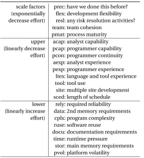
scale factors prec: have we done this before? (exponentially flex: development flexibility decrease effort) resl: any risk resolution activities?
team: team cohesion pmat: process maturity upper acap: analyst capability (linearly decrease pcap: programmer capability
effort) pcon: programmer continuity aexp: analyst experience pexp: programmer experience
ltex: language and tool experience tool: tool use
site: multiple site development sced: length of schedule
lower rely: required reliability
(linearly increase data: 2nd memory requirements effort) cplx: program complexity
ruse: software reuse
docu: documentation requirements time: runtime pressure
stor: main memory requirements pvol: platform volatility
Figure 5.1Descriptions of the XOMO variables.
ranges values project feature low high feature setting
rely 3 5 tool 2
FLIGHT: data 2 3 sced 3
cplx 3 6
JPL’s flight time 3 4
software stor 3 4
acap 3 5
apex 2 5
pcap 3 5
plex 1 4
ltex 1 4
pmat 2 3
KSLOC 7 418
rely 1 4 tool 2
GROUND: data 2 3 sced 3
cplx 1 4
JPL’s ground time 3 4
software stor 3 4
acap 3 5
apex 2 5
pcap 3 5
plex 1 4
ltex 1 4
pmat 2 3
KSLOC 11 392
prec 1 2 data 3
OSP: flex 2 5 pvol 2
resl 1 3 rely 5
Orbital space team 2 3 pcap 3
plane nav& pmat 1 4 plex 3
gudiance stor 3 5 site 3
ruse 2 4
docu 2 4
acap 2 3
pcon 2 3
apex 2 3
ltex 2 4
tool 2 3
sced 1 3
cplx 5 6
KSLOC 75 125
prec 3 5 flex 3
OSP2: pmat 4 5 resl 4
docu 3 4 team 3
OSP ltex 2 5 time 3
version 2 sced 2 4 stor 3
KSLOC 75 125 data 4
pvol 3 ruse 4 rely 5 acap 4 pcap 3 site 6
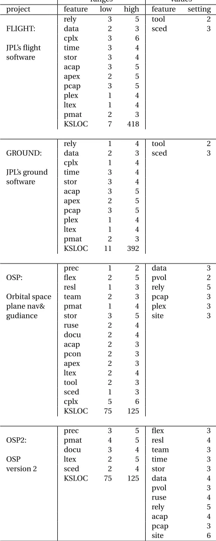
5.2.1 Benchmarks of XOMO
XOMO, introduced in[MR05], is a general framework for Monte Carlo simulations that combine four COCOMO-like software process models from Boehm’s group at the University of Southern California. Figure 5.1 lists the description of XOMO input variables (All should be within[1, 6]). The XOMO user begins by defining a set ofrangesor a specificvalueof these variables to address his or her real situation in one software project. For example, if the project has (a)relaxed schedule pressure, they should setscedto its minimal value; (b)reduced functionalists, they should halve the value ofklocand minimize the size of the project database (by settingdata=2); (c)reduced quality (for racing something to market), they might move to lowest reliability, minimize the documentation work and the complexity of the code being written, reduce the schedule pressure to some middle value– in the language of XOMO, this last change would berely=1, docu=1, time=3, cplx=1.
XOMO computes four objective scores: (1) projectrisk; (2) developmenteffort; (3) predicted defects; (4) totalmonthsof development. Effort and defects are predicted from mathematical models derived from data collected from hundreds of commercial and Defense Department projects[Boe00]. As to theriskmodel, this model contains rules that trigger when management decisions decrease the odds of completing a project: e.g., demandingmorereliability (rely) whiledecreasinganalyst capability (acap). Such a project is “risky” since it means the manager is demanding more reliability from less skilled analysts. XOMO measuresriskas the percent of triggered rules.
The optimization goals for XOMO are to:
1. Reduce risk;
2. Reduce effort;
3. Reduce defects;
4. Reduce months.
Note that this is a non-trivial problem since the objectives listed above as non-separable and con-flicting. For example,increasingsoftware reliabilityreducesthe number of added defects while increasingthe software development effort. Also,moredocumentation can improve team commu-nication anddecreasethe number of introduced defects. However, such increased documentation increasesthe development effort. Consequently, XOMO is multi-objective optimization problem. MOEA algorithms can handle this.[Kra15a]and[Lek14]pointed out that the NSGA-II[Deb00b]can solve this problem and return quite good results. In our experiments, we will compare SWAYwith the NSGA-II algorithm in solving XOMO cases.
In our case studies with XOMO, we use four scenarios taken from NASA’s Jet Propulsion Labora-tory[Men09b]. As shown in Figure 5.2, FLIGHT and GROUND are general descriptions of all JPL flight and ground software while OSP and OPS2 are two versions of the flight guidance system of the Orbital Space Plane.
Short name Decision Description
Cult Culture Number (%) of requirements that change. Crit Criticality Requirements cost effect for safety critical
sys-tems.
Crit.Mod Criticality Modifier Number of (%) teams affected by criticality. Init. Kn Initial Known Number of (%) initially known requirements. Inter-D Inter-Dependency Number of (%) requirements that have
interde-pendencies to other teams.
Dyna Dynamism Rate of how often new requirements are made. Size Size Number of base requirements in the project. Plan Plan Prioritization Strategy: 0= Cost Ascending;
1= Cost Descending; 2= Value Ascending; 3=Value Descending; 4= C o s t
V a l u e Ascending.
T.Size Team Size Number of personnel in each team
Figure 5.3List of inputs to POM3. These inputs come from Turner & Boehm’s analysis of factors that con-trol how well organizers can react to agile development practices[BT03b].
POM3a POM3b POM3c
A broad space of projects.
Highly critical small projects
Highly dynamic large projects Culture [0.10, 0.90] [0.10, 0.90] [0.50, 0.90] Criticality [0.82, 1.26] [0.82, 1.26] [0.82, 1.26] Criticality Modifier [0.02, 0.10] [0.80, 0.95] [0.02, 0.08] Initial Known [0.40, 0.70] [0.40, 0.70] [0.20, 0.50] Inter-Dependency [0.0, 1.0] [0.0, 1.0] [0, 50]
Dynamism [1, 50] [1.0, 50.0] [40, 50]
Size [30, 100] [3, 30] [30, 300]
Team Size [1, 44] [1, 44] [20, 44]
Plan [0, 4] [0, 4] [0, 4]
Figure 5.4Three specific POM3 scenarios.
space of the cases, we have
OSP≈OSP2<GROUND<FLIGHT (5.1)
5.2.2 Benchmarks of POM3, a Model of Agile Development
POM3 model is a tool for exploring the management challenge of agile development[BT03b; Por08; BT03a]– balancingidle rates,completion ratesandoverall cost. More specifically,
• In the agile world, projects terminate after achieving acompletion rateofX%(X <100)of its required tasks;
![Figure 5.3 List of inputs to POM3. These inputs come from Turner & Boehm’s analysis of factors that con-trol how well organizers can react to agile development practices [BT03b].](https://thumb-us.123doks.com/thumbv2/123dok_us/1620528.1201417/42.612.104.525.311.479/figure-turner-boehm-analysis-factors-organizers-development-practices.webp)