Rose-Hulman Institute of Technology
Rose-Hulman Scholar
Graduate Theses - Engineering Management
Engineering Management
3-2018
Trajectory Generation and Control of a Mobile
Robot for Radar Target Simulation
Anthony Michael Adamo
Follow this and additional works at:
https://scholar.rose-hulman.edu/
dept_engineering_management
Part of the
Systems Engineering Commons
This Thesis is brought to you for free and open access by the Engineering Management at Rose-Hulman Scholar. It has been accepted for inclusion in Graduate Theses - Engineering Management by an authorized administrator of Rose-Hulman Scholar. For more information, please contact
Recommended Citation
Adamo, Anthony Michael, "Trajectory Generation and Control of a Mobile Robot for Radar Target Simulation" (2018).Graduate Theses - Engineering Management. 1.
Trajectory Generation and Control of a
Mobile Robot for Radar Target Simulation
Anthony Adamo
Rose-Hulman Institute of Technology Hochschule Ulm
Thesis submitted for the degree of
Masters of Systems Engineering and Engineering Management
Declaration of Authorship
I hereby declare that this thesis is entirely the result of my own work except where otherwise indicated.
I have only used the resources given in the list of references.
Signed:
Date:
Anthony Michael Adamo
M.Sc.Eng. Systems Engineering and Engineering Management Ulm, Baden-W¨urttenberg.
Abstract
This thesis presents a straight forward method for developing time-dependent trajectories with smooth paths for mobile robots. Cubic Bezier curves are utilized to efficiently generate segments of complex paths with associated linear and angular velocity profiles. The speeds along the path are planned considering the kinematic and dynamic constraints of a typical differential drive mobile robot. A PID controller was developed to control for both path following and the timing constraints of the generated trajectories. This research was developed to aid in the KoRRund project in testing their radar system’s accuracy in detecting objects at a specific time and space and their measured velocity. These readings would then be compared to the known trajectory of the mobile robot. The AGV mobile robot developed by InMach and Adlatus Robotics was used in the physical testing of this research.
Acknowledgments
During the six months I had the pleasure of working in a supportive and helpful environment at InMach. My colleagues were very friendly and always available to help me every step of the way.
I would first like to thank my university advisers Dr. Moore and Dr. Bank for not only convincing me to enroll in the SI program, but for being supportive and helpful throughout my studies. Another thanks to Dr. Bank for putting me in touch with the great people at InMach in the first place. Without both of your help and guidance, none of this would be possible.
Next I would like to thank my work adviser Borris Kluge for being such a an amazing resource for insight and technical knowledge. Your knowledge of the theoretical aspects and your ability to put them into practice was immensely helpful throughout the process. I must also thank my other work adviser Siegfried Hochdorfer for his help in many of the technical aspects of the robotic framework.
Special thanks Manuel Freudenreich for his patience and genuine interest in the progression of my work. You were always able to take time away from your tasks to help me with all of the intricacies of the project’s software, hardware, and framework. Without your knowledge and availability I am not sure I would have been able to do any actual testing.
Finally, I would like to thank all of my friends and family for their support and motivation throughout the entirety of my endeavor.
Contents
1 INTRODUCTION 1
1.1 Purpose of Research . . . 1
1.2 Related Work . . . 1
2 TRAJECTORY GENERATION 3 2.1 Curve and Path Definitions . . . 3
2.2 Bezier Curve Generation . . . 4
2.3 Speed/Timing Profile . . . 10
2.4 Nominal Paths for Testing . . . 15
3 ROBOTIC FRAMEWORK AND CONTROLLER DESIGN 21 3.1 Robot Hardware . . . 21
3.2 Robot Component Framework . . . 23
3.3 Controller Design . . . 25
4 SIMULATION TEST RESULTS 31 4.1 Simulation Environment . . . 31
4.2 Simulation Results - Basic Curve . . . 32
4.3 Simulation Results - Figure 8 Path . . . 37
4.4 Simulation Results - Oval Path . . . 40
4.5 Simulation Results - Square Path . . . 43
4.6 Simulation Results with Multiple Laps . . . 46
5 PHYSICAL ROBOT TEST RESULTS 55 5.1 Physical Robot Transition . . . 55
5.2 Test Results - Figure 8 Path . . . 56
5.3 Test Results - Oval Path . . . 59
5.4 Test Results - Square Path . . . 62
6 CONCLUSION AND FUTURE WORK 67 6.1 Conclusion . . . 67
Chapter 1
INTRODUCTION
1.1
Purpose of Research
The purpose of this research is to create a way to generate trajectories consisting of smooth complex paths with timing/speed profiles and execute these trajectories on a mobile robot. The ability to do this will allow for testing the accuracy of a radar system to detect objects at a specific time and space with a measured speed, and compare these readings to the object’s actual taken path and timing/speed profile. The company InMach is partners on the project KoRRund which aims at developing a ”Conformal and multistatic MIMO radar configuration for all-round view for autonomous driving”. In the testing of this radar there needs to be targets that can emulate the motion of common obstacles an autonomous car might encounter such as a pedestrian walking or a bicyclist. For an autonomous car to be as safe as possible, it must not only identify the targets, but it must identify their Cartesian location, their direction of motion, and the speed at which they are traveling at. The aim of this project is to create a method for a mobile robot to move along a specific path with a specific speed and direction so that the accuracy of this radar can be detected. If it is possible to know that a time t, the robot was at (x, y) location moving in the theta direction with velocityv, the reading at this time from the radar could then be compared for accuracy and effectiveness.
1.2
Related Work
Trajectory generation and following are not new topics in mobile robotics. Many approaches and mathematical techniques have been used to generate trajectories with paths from many different path families, with and without smooth curvature. One of the earlier pieces that I researched, ”Robot Motion Planing and Control”, dates back to 1998. In the fourth chapter of this book titled ”Feedback Control of a Nonholonomic Car-Like Robot” they discuss the difference in feedback control approaches from a point to point motion task, a path following motion task, and a trajectory tracking motion task. ”In the trajectory tracking task, the robot must follow a desired Cartesian path with a specified timing law(equivalently, it must track a moving reference robot)”. They discuss the possibility of separating the geometric path from the timing law which is not necessary and was not done in this thesis. In this thesis the timing law was merely the time evolution for the desired position of the robot in the path. They go into detail about the introduction ofN trailers into the robot design and
how to account for stabilization. The chapter also goes into the kinematic calculations for wheel rotations and how to model the control inputs into a simple linear velocity and angular velocity inputs/outputs. These calculations and relations have already been implemented in InMach’s robot framework so this area of the chapter was not necessary to further my work in the project.
In the initial phase of the research it needed to be decided which family of paths would be chosen to generate the paths of the trajectories. The decision between parametric and polynomial curves became apparent early on. In the paper ”Time-dependent Motion Planning for Nonholonomic Mobile Robots” they use polynomial curves instead of using Bezier curves due to their approach for introducing timing profiles into the trajectory. In this paper they account for obstacle avoidance and therefor have a set timing for begin and end point, but do not have a strict path that needs to be followed due to this feature. Since the object of this thesis is to have a robot that can emulate targets for a radar detection system and be at a specific time and place with a specific speed, the inclusion of obstacle avoidance and deviation from the set path is completely against the functional requirements of the work.
The most similar article to the work done in this project was published in the International Journal of Control and Automation in 2013 titled ”Smooth Trajectory Planning Along Bezier Curve for Mobile Robots with Velocity Constraints”. In this paper they produce an S-Curve path using a cubic Bezier curve and add velocity constraints using convolution operators. The use of Bezier curves is the same as in the work of this thesis, although this thesis takes it further by concatenating multiple cubic bezier curves to create more complex and continuous paths that can have multiple laps. The main deviation between this article and the work in this thesis however is the introduction of time into the trajectory generation. In the article, Yang and Choi use a square wave and convolve it with the bezier path to create a timing profile based on multiple velocity points(vinitial, vf inal, vmax).
In adding a timing profile to the generated path, the use of a ”Bang Bang” style of acceleration was considered. The ”Bang Bang” style of acceleration is a very simple way to implement velocity and position into a point to point motion task. The idea and calculations for this was gone into detail in the Trajectory Planning in Cartesian Space lecture Slides from Professor Allesandro De Luca at the Universita Di Roma. In these slides Professor De Luca discusses the timing law associated with the Bang Bang style and how to incorporate this with any predefined Cartesian path. This style was originally the approach to be used in this thesis before the method of incorporating velocity as a third dimension in the Bezier curve was made apparent.
Chapter 2
TRAJECTORY GENERATION
2.1
Curve and Path Definitions
The initial challenge was to find a way to define smooth paths to minimize energy and travel time. After researching many articles, books, and other academic documents, most of the smooth path generation methods used in mobile robots seemed to incorporate cubic B´ezier and Beta-Spline(B-Spline) curves. Both curves create paths with constant curvature using a set of control points which have weight on the overall curve’s path. Below in Figure 2.1 is an example of a cubic B-Spline with 6 control points and a cubic Bezier with 4 control points.
(a) cubic B-Spline Curve (b) cubic Bezier Curve
Figure 2.1: Examples of cubic B-Spline and cubic Bezier curves
The major of drawback of B-Spline curves arises in the complexity of coding vs the benefits gained compared to a Bezier in this specific application. The major drawback of Bezier curves arises when making more complex paths with multiple changes in direction. To change direction in either format, it is necessary to add in another control point, and adding control points in a Bezier increases the the overall degree of the polynomials. A Bezier curve with u control points can effectively have u−1 changes in direction and will have u−1 degree polynomials. B-Spline Curves do not have this inherent property, so adding control points does not affect the overall degree of the polynomials. However, it is possible to join together multiple Bezier curves from tail-to-head by concatenating the last control point of one curve with the beginning control point of another. Using this method it is possible to make more complex paths by simply segmenting it out into multiple cubic bezier curves.
2.2
Bezier Curve Generation
For computational simplicity and path complexity the method of connecting multiple cubic Bezier curves was chosen. Each segment curve is calculated using defined ”Base” functions and given an input of an initial point Pi(A0, B0), final point Pf(A3, B3), and control points
C1(A1, B1) and C2(A2, B2). The two control points are the values that pull the curve away
from being a straight line between initial point and end point.
The Base equations of a cubic bezier curve for generating x and y values are
x(u) = (1−u)3A0+ 3u(1−u)2A1+ 3u2(1−u)A2+u3A3 (2.1)
y(u) = (1−u)3B0+ 3u(1−u)2B1+ 3u2(1−u)B2+u3B3 (2.2)
In equations 2.1 and 2.2, the value of (u) is arbitrary and can be any value 0 ≤ u ≤ 1 in increasing order to generate a smooth curve from initial point to final point. For a more precise Bezier curve with small increases from point to point, amount ofu points should be increased. In this report, there are 1000u points for each cubic Bezier segment. The values generated in equation 2.1 and 2.2 do not consider time are are only parameterized byupoints. An illustration of the results of equations 2.1 and 2.2 is given below in figure 2.2
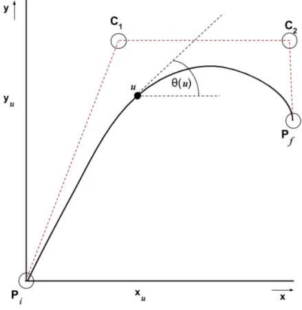
Figure 2.2: Cartesian representation of a cubic Bezier curve
To find the tangent angleθ(u) at any point of the curve, we can take the first derivative of the Cubic Bezier curve and then use the inverse tangent
x0(u) = 3(1−u)2(A1−A0) + 6u(1−u)(A2−A1) + 3u2(A3−A2) (2.3)
θ(u) = arctan y0(u) x0(u) (2.5) An illustration of incorporating tangent angleθ(u) to the curve description is given below in figure 2.3.
Figure 2.3: Representation of a cubic Bezier curve with tangent angles
To find the curvatureκ(u) at any point of the curve, we can take the second derivative of the base cubic Bezier equations and use the values in the nominal curvature formula shown equation 2.8:
x00(u) = 6(1−u)(A2−2A1+A0) + 6(A3−2A2+A1) (2.6)
y00(u) = 6(1−u)(B2−2B1+B0) + 6(B3−2B2+B1) (2.7)
κ(u) = x
0(u)y00(u)−y0(u)x00(u)
(x0(u)2+y0(u)2)3/2 (2.8)
A feature of curvature is that it can also be defined as the reciprocal of the radius of a circle at the given point u.
κ(u) = 1
Figure 2.4: Representation of a cubic Bezier curve with curvature
An illustration of incorporating curvature κ(u) to the curve description is given below in figure 2.4.
At this point the path can be defined as:
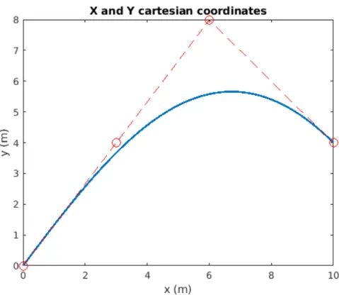
C(u) = [x(u), y(u), θ(u), κ(u)] This was all implemented in MATLAB with the initial points:
Pi= [ 0.0,0.0 ]
C1 = [ 3.0,4.0 ]
C2 = [ 6.0,8.0 ]
Figure 2.5: Cartesian representation of the cubic Bezier curve in MATLAB
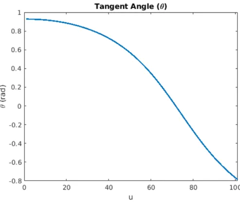
Figure 2.6: Tangent angle of the cubic Bezier curve in MATLAB
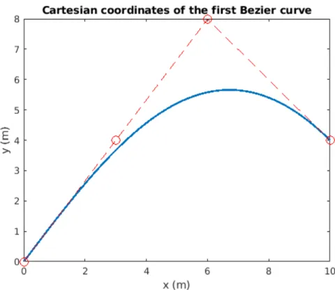
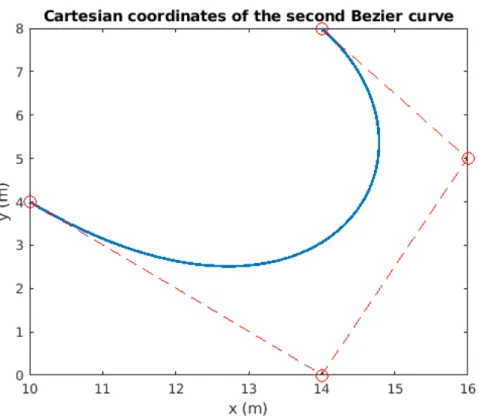
To create a Composite Bezier curve by combining two or more Bezier curves, the initial point(Pi) of the second curve must be equal to the final point(Pf) of the first curve. With
this condition satisfied, one can make complex paths by concatenating any number of Bezier curve segments. An example of this is shown in Figures 2.8 through 2.10 using the points:
Pi,0 = [0.0,0.0 ] Pi,1 = [10.0,4.0 ]
C1,0 = [3.0,4.0 ] C1,1 = [14.0,0.0 ]
C2,0 = [6.0,8.0 ] C2,1 = [16.0,5.0 ]
Figure 2.8: Cartesian representation of the first cubic Bezier curve in MATLAB
Figure 2.9: Cartesian representation of the second cubic Bezier curve in MATLAB
2.3
Speed/Timing Profile
At this point the trajectory has a clearly defined path but has no values for time, velocity, or acceleration associated with it. The previous values and graphs ofx(u), y(u), θ(u),andκ(u) are still not a function of time(t), but a function of points along the curve(u).
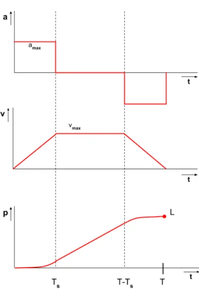
Initially, using a ”bang-coast-bang” acceleration format was considered as a way to incorpo-rate time, velocity, and acceleration. A ”bang-coast-bang” format has a constant acceleration until the robot reaches a specific velocity, then the robot would hold that velocity for the ”coasting” period, and then finally have a negative ”bang” acceleration for the same duration as the initial acceleration period.
The equations for incorporating position and time are provided below in equations 2.9-2.11. The relevant variables in these equations are: max acceleration(amax), velocity maximum(vmax),
distance traveled(L), current time(t), initial time(T0), time to start the coast(Ts), and final
time(Tf). (T0 < t < Ts) : p(t) =amax t2 2 (2.10) (Ts< t < Tf −Ts) : p(t) =vmaxt− vmax2 2amax (2.11) (Tf −Ts < t < Tf) : p(t) =−amax (t−Tf)2 2 +vmaxt− v2max amax (2.12)
Figure 2.11: Bang-Coast-Bang acceleration format
Above in Figure 2.8 is an illustration of a Bang-Coast-Bang timing/speed profile Upon further research it became apparent that it is possible to incorporate time, velocity, and acceleration into the trajectory description by adding a third dimension to the point vectors. Therefor, each point for the cubic bezier curve is in the format.
Pi = [Ai, Bi, Ci]
This allows for more dynamic velocity and acceleration information at each point along the standard bezier curve. The velocity and acceleration graphs as a function of curve parameter (u) are provided below in figure 2.12 using the points:
Pi = [0.0,0.0,0.0]
C1= [3.0,4.0,0.3]
C2= [6.0,8.0,0.9]
Figure 2.12: Velocity of the cubic Bezier curve in MATLAB
The trajectory vector is now in the form:
C(u) = [x(u), y(u), θ(u), κ(u), v(u), a(u)]
Using the velocity parameter, it is possible to introduce time into the curve and finally have an associated time at each curve parameter. This is done with the simple definition of velocity
v= distance time
To find distance we will find the arc lengthS(u) from one pointito the nexti+ 1. Since the curve is densely populated with 1000 (u) points, we can accurately estimate arc length by using the Pythagorean theorem since the distance of the curve that is cut off is negligible. So the arclength S(u) is calculated with the equation:
S(u) =p(x(u+ 1)−x(u))2+ (y(u+ 1)−y(u))2 (2.13)
Figure 2.14: Arc length between points u and u+1
Using arc length as the distance, it is now possible to calculate the value of time for each point (u). By using the average velocity between u andu+ 1
vavg(u) =
v(u) +v(u+ 1) 2
time is easily computed for each u.
t(0) = 0 t(u+ 1) = S(u) vavg(u) or t(u+ 1) = 2 S(u) v(u) +v(u+ 1) (2.14)
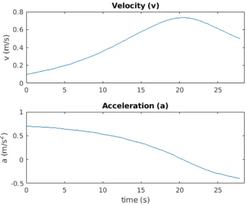
With time incorporated it is now possible to generate much more useful graphsv(t), a(t), θ(t), and κ(t)
Figure 2.15: Velocity and acceleration vs. time in MATLAB
After successfully implementing time into our trajectory definition, the final form of our trajectory vector is:
C(u) = [x(u), y(u), θ(u), κ(u), v(u), a(u), t(u) ]
2.4
Nominal Paths for Testing
Before moving on to simulations and testing with the physical robot, three continuous paths that allow for lapping were created. These paths were chosen to test for generality and accuracy of the trajectory controller. The three paths chosen are an oval, a square, and a figure 8. Both the oval and figure 8 test long sweeping turns, the square tests for sharp turns, and the figure 8 tests left and right turns in one single path.
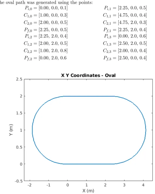
The oval path was generated using the points:
Pi,0 = [0.00,0.0,0.1] Pi,1 = [2.25,0.0,0.5] C1,0 = [1.00,0.0,0.3] C1,1 = [4.75,0.0,0.4] C2,0 = [2.00,0.0,0.5] C2,1 = [4.75,2.0,0.3] Pf,0 = [2.25,0.0,0.5] Pf,1 = [2.25,2.0,0.4] Pi,2 = [2.25,2.0,0.4] Pi,3 = [0.00,2.0,0.6] C1,2 = [2.00,2.0,0.5] C1,3 = [2.50,2.0,0.5] C2,2 = [1.00,2.0,0.8] C2,3 = [2.00,0.0,0.4] Pf,2 = [0.00,2.0,0.6 Pf,3 = [2.50,0.0,0.4]
Figure 2.18: Velocity of the oval shaped path in MATLAB The square path was generated using the points:
Pi,0= [0.00,0.00,0.2] Pi,1 = [1.25,1.25,0.2] C1,0= [1.25,0.00,0.3] C1,1 = [1.25,2.50,0.2] C2,0= [1.25,0.00,0.3] C2,1 = [1.25,2.50,0.2] Pf,0= [1.25,1.25,0.2] Pf,1 = [0.00,2.50,0.1] Pi,2= [ 0.00,2.50,0.1] Pi,3 = [−1.25,1.25,0.4] C1,2= [ −1.25,2.50,0.3] C1,3 = [−1.25,0.00,0.2] C2,2= [ −1.25,2.50,0.4] C2,3 = [−1.25,0.00,0.2] Pf,2= [ −1.25,1.25,0.4] Pf,3 = [ 0.00,0.00,0.1]
Figure 2.19: Cartesian representation of the square shaped path MATLAB
The figure 8 path was generated using the points: Pi,0 = [0.00,0.00,0.1] Pi,1 = [2.25,2.00,0.5] C1,0 = [0.75,0.50,0.2] C1,1 = [4.50,3.00,0.3] C2,0 = [1.50,1.50,0.4] C2,1 = [4.50,−1.0,0.2] Pf,0 = [2.25,2.00,0.5] Pf,1 = [2.25,0.00,0.2] Pi,2 = [2.25,0.00,0.2] Pi,3= [0.00,2.00,0.5] C1,2 = [1.50,0.50,0.4] C1,3= [−2.25,3.00,0.3] C2,2 = [0.75,1.50,0.5] C2,3= [−2.25,−1.0,0.2] Pf,2 = [0.00,2.00,0.5] Pf,3= [0.00,0.00,0.1]
Chapter 3
ROBOTIC FRAMEWORK AND
CONTROLLER DESIGN
3.1
Robot Hardware
The basic framework used in this project is written in C++ and based on the CR700 cleaning robot produced and developed by InMach and Adlatus. The CR700 is an industrial wet floor cleaning robot used primarily in grocery stores and large factories. The physical robot used in the tests is a differential drive shopping cart robot designed for use in the popular German supermarket chain Kaufland. This robot has the same drive motors, laser scanner, inertial measurement unit (IMU), master and slave computers, and batteries as the CR700 cleaning robot that the framework was developed for. An Image of the shopping cart is shown in Figure 3.1 and a block definition diagram of the physical components is provided in Figure 3.2.
3.2
Robot Component Framework
The CR700 framework has a simplified system for sending and receiving sensor data and drive commands called Simple Application Messaging (SAM). The SAM system has many sub-components encompassing the robot’s kinematic equations, laser scanner interpretation, odometry calculations, IMU information, self localization, and simplified drive commands. Each of these components are generalized so that the only necessary changes when switching from the simulated robot to the physical robot are the port connections. The kinematic equations are done in part with the simplified drive commands so that the only necessary inputs to drive the robot are linear velocity (v) and angular velocity (ω) values. As stated before, the generated trajectory vector has a linear velocity value at every point along the curve, but it does not have an angular velocity value at each point. Therefor, it is necessary to calculate it for each point on the curve to have a fully defined nominal trajectory vector. The angular velocity can be calculated with Equation 3.1.
ω= v
r (3.1)
Using the definition of κas the inverse radius shown in Equation 2.9, the calculation forω(u) can be done simply by multiplying v(u) and κ(u) at each point along the curve.
ω(u) =v(u)∗κ(u) (3.2)
Adding theseω(u) values gives us the final form of the trajectory vector that will be supplied to the trajectory controller.
C(u) = [x(u), y(u), θ(u), κ(u), v(u), ω(u), t(u) ]
InMach has a well developed simulation environment for the CR700 using the Modular OpenRobots Simulation Engine (MORSE). Developed by OpenRobots, MORSE is an generic simulator for academic robotics. It focuses on realistic 3D simulation of any environment large or small and can consist of multiple robots being simulated at once. MORSE comes with a set of standard sensors and actuators and the ability to edit them to create an accurate representation of a robot’s actual sensors and actuators. Although the only sensors used in this project were odometric and laser scanners, InMach had already modeled them for the CR700. MORSE rendering is based on the Blender Video Game Engine meaning that a more powerful computer is necessary to run simulations.
MORSE is the base simulator which sends the laser scanner, odometry, and IMU infor-mation to the SAM components. These messages are received and sent to a pose tracker component which provides the current position and orientation data read by the trajectory controller. The positional updates from MORSE are interpreted as geometry messages within the SAM system and represented in Quaternion notation. Since the trajectory vector is not in Quaternion notation, the yaw is necessary to be calculated to compare the current robot direction θr and the nominal tangent angle θn. The simple functional flow diagram for the
simulation process and how information is sent between the controller and robot is shown in Figure 3.3.
Figure 3.3: Simple functional flow diagram
Also in Figure 3.3, the trajectory generator component is done separately before initializing the robot and the trajectory controller. The trajectory component reads in the generated trajectory values then tells the simulator its initial position, orientation, and velocities. Once this initialization is completed the robot will begin to move and the pose tracker will begin to send time stamped position and orientation updates.
While this is a very basic view of how information is shared between the layers of the system, the SAM components are much more complex. There are four components used in the self localization process before the trajectory controller receives any positional updates. The Montecarlo Localization component uses the robot’s odometry and laser scanner data in a particle filter to give the most accurate localization data, but is only available every 66.66ms due to the slower refresh rate of the laser scanner. The Extended Odogyrometry component takes the odometry and IMU data for localization updates available every 20ms but is less accurate than the Montecarlo updates. Both of these component’s data is fed into the Pose Tracker component which weighs them and provides the trajectory controller with positional updates every 20ms on average with an accuracy of 5 cm. Upon receiving a positional update message, the trajectory controller component is triggered and uses the data to calculate the appropriate drive commands to be sent to the robot to follow the trajectory accurately. A more detailed view of the component interactions is shown in Figure 3.4.
Figure 3.4: Detailed messaging architecture
3.3
Controller Design
Given the time stamped position and orientation updates, there was a decision to make on what style of controller should be used to follow the generated trajectory. Some research was done on more traditional proportional–integral–derivative (PID) controllers or a more complex state-based methods such as a Model Predictive Controller (MPC).
PID controllers are very simple in nature, they are feedback loops based on continuous error calculations e(t) between a nominal value and measured value. These error values are then used to apply corrections to the system input in proportional, integral, and derivative
terms. These controllers are widely used in many fields and are among the most simple control methods. An illustration of a PID controller feedback loop can be seen in Figure 3.5.
Figure 3.5: PID controller feedback loop
An MPC is an advanced and complex method of process control used most in the repre-sentation of dynamical systems. MPC’s are able to optimize the current state of a process while incorporating future states in the model. This is done by constantly optimizing your current state and reevaluating your future states each step of the way. They have the ability to take measured control actions based on future events, an ability that PID controllers do not have. This is the main advantage over PID controllers. A basic illustration of an MPC is provided in Figure 3.6.
Figure 3.6: MPC controller feedback loop
It quickly became apparent that in the scope of this project, the NMPC controller is unnecessarily complex. The additional benefits in accuracy are not substantial compared to a PID controller in such a simple system . Therefor, the decision was made to develop a simple P controller using the orthogonal distance, vector angular difference, and time difference calculated earlier.
Each position and orientation message is used to calculate the closest nominal point on the curve to the robot. Once the closest nominal point on the curve is found, one can define a local coordinate frame on the robot instead of using only the world frame. To do this, it is advantageous to work with vectors. The vector quantities used are: nominal position (pn)
and direction (an), and robot’s position (pr) and direction (ar). These are defined below in
vector form:
position: p= [x, y]
direction: a= [cos(θ),sin(θ)]
Since the path is densely populated with points, using the Pythagorean theorem to calculate the distance between the robot and the closest point is useful to find the robot’s distance from the path. However using the Pythagorean theorem does not utilize the robot’s local coordinate frame and therefor does not provide information about the robot’s position relative to the path. To incorporate the robot’s local coordinate frame one can find the perpendicular distance(dy) between the robot’s vector and the closest point’s vector. This distance is signed,
so a positive distance indicates that the path is to the right of the robot and a negative distance indicates that the path is to the left. Below in Figure 3.7 is a graphic showing the relationship between these values. The relevant variables are the closest point(u), distance from closest point(dcp), perpendicular distance(dy), and parallel distance(dx).
Figure 3.7: Diagram for perpendicular distance
The perpendicular distance (dy) and parallel distance (dx) can be calculated with the following
formulas in Equations 3.3 and 3.4.
dy =an×(pr−pn) (3.3)
dx =an•(pr−pn) (3.4)
These distance values are not the only advantageous for finding the distance from the path, they can also be used to find the angular difference (∆θ) between the tangent angle at
the closest point (θ(u)) and the orientation of the robot (θr). An image showing the angular
relationship between the two vectors is provided in Figure 3.7.
Figure 3.8: Diagram for vector angular difference
Calculating the angular difference (∆θ) can be done with the atan2 function in C++ using the perpendicular and parallel distances as inputs.
∆θ= atan2(dy, dx) (3.5)
Both the perpendicular distance (dy) and angular difference (∆θ) are used as control
variables for the steering the robot back to the nominal path. In the implementation of the P controller, they are used only to control the angular velocity commands (ωcmd) sent to the
robot. Without controlling for time, the angular velocity command is calculated in Equation 3.6.
ωcmd=ω(u)−Kdist∗dy −Ktheta∗∆θ (3.6)
To control for the speed/timing profile it is necessary to regulate both the angular and the linear velocity of the robot with respect for time. To introduce this timing difference into the system, the time-stamped positional updates from the robot (trobot) and the nominal
time associated with the closest point found on the curve (tnom) need to be associated. This
difference (∆t) is just a simple subtraction between the two values.
∆t=t(u)−trobot (3.7)
Using the nominal linear velocity at the closest point (v(u)), the ∆t value is used to adjust the linear velocity and control for timing errors associated with the parallel distance between the robot and the closest point (dx). This control value will be subtracted from the nominal
linear velocity to create a linear velocity command sent to the robotvcmd.
vcmd =v(u)−Ktime∗∆t (3.8)
As stated previously, the calculation of the angular velocity command in equation 3.6 does not incorporate time into the system. Time can be incorporated by using the newly calculated vcmd as the velocity used in Equation 3.2 instead of the nominal linear velocity at the closest
pointv(u).
This time dependent angular velocity is then used instead of the nominal angular velocity in equation 3.6 to produce the actual angular velocity command sent to the robot
Chapter 4
SIMULATION TEST RESULTS
4.1
Simulation Environment
Setting up the MORSE simulator was quite a time consuming and difficult task. It is a powerful and complex tool which requires quite a lot of research and knowledge to set up. Thankfully InMach has already developed a 3D model of a differential drive robot and have implemented all of the sensors for the CR700. Along with their robot, they have developed multiple maps to simulate various environments such as a supermarket layout or a factory floor. An open world map with parallel rows of landmarks was used in the testing of the trajectory control component. Below in Figure 4.1 is a screen capture of the top view of the simulated robot in the open world map in MORSE. One thing to be noted, the initial position of the robot is at (0,0) and the initial orientation is at 0 radians.
Figure 4.1: Screen capture of MORSE simulation environment
The main benefit to running simulations before moving to the actual robot was the ability to identify fundamental issues between the theoretical research and the implementation of the controller design, SAM messaging protocols, and tuning the control constants. The first goal was to follow the path with no time constraints using nominal velocity. To achieve proper path following requires tuning the control constantsKdist and Ktheta.
MATLAB was used to visualize the path taken compared to the nominal path, and to identify patterns in the data received from the position and orientation messages. The nom-inal path used in initial testing had a total time of 43.063 seconds. The SAM pose-tracker component sends roughly 50 timestamped messages with position and orientation per sec-ond. This means that there are roughly 2,150 data points received throughout the entirety of the path. These messages were formatted and written to a csv file and interpreted with MATLAB.
4.2
Simulation Results - Basic Curve
A basic Bezier curve was used for developing the controller and tuning the control constants. This basic path was generated using the points:
Pi = [0.0,0.0,0.10]
C1= [3.0,4.0,1.00]
C2= [6.0,8.0,0.75]
Pf = [13.0,4.0,0.10]
Figure 4.2: Nominal path used for tuning control constants - Basic curve
Due to the initial orientation of 0 radians and the initial tangent angle of the nominal path being 0.927 radians, the trajectory controller will quickly rotate the robot to align within 0.2 radians before moving forward with the path following. This orientation adjustment will affect the position and timing errors in this initial test case. A graph of the simulated path vs nominal path is shown below in Figure 4.3 and a graph of the distance error is provided in Figure 4.4. The basic curve trajectory was implemented with a P controller using the control constants:
Ktime = 0.01
Kdist= 90.0
Figure 4.3: XY comparison - Basic curve
The robot was able to follow the path within an accuracy of 3.44cm at the furthest point, and an average distance error of 0.56cm throughout the entirety of the path. The distance error in Figure 4.4 was calculated using he Pythagorean theorem and the closest point found, therefor all values are positive. As discussed earlier, this distance calculation is not as useful as the perpendicular distance from the tangent line of the closest point found (dy). This distance will
give both positive and negative values get positive and negative results which shows whether the robot is over-correcting and staying inside the path, under-correcting and staying outside the path, or more properly correcting and wiggling from side to side of the path. A graph of the perpendicular distance error for the basic path is provided below in Figure 4.5. This perpendicular distance value will be used for all distance error graphs throughout the rest of this report.
Figure 4.5: Perpendicular distance error in MORSE - Basic curve
The next step was in developing the controller was to adjust for the timing/speed profile by tuning the control constantKtime. Since there are 2,150 messages received over the 1000u
points, there is an average of 2.15 messages for eachupoint, each with different time stamps. To analyze the timing data, it was necessary to average the values for each data point received to come to a proper estimation of when the robot was actually closest the point reported, instead of slightly behind or in front of it. These average values were compared to the nominal timing values to produce the graphs in Figures 4.6 and 4.7.
Figure 4.6: Timing comparison - Basic curve
The maximum time error that occurs in the path is 32.277ms, and an average average of -0.1305ms. The absolute value of the time error throughout the path is 4.088ms. Due to the positional updates arriving every 20ms, the accuracy of the speed profile is well within the range of error to be expected in such a system.
Given that the model of the CR700 has a maximum linear and angular velocity of 0.8m/s, the maximum distance error that can be attributed to being either behind or ahead of schedule is 2.582cm. This is well within range of the error to be expected from localization.
4.3
Simulation Results - Figure 8 Path
Based on these results from following the basic path, the controller was deemed to be accurate enough to move on to implementing and testing the three continuous paths that were described previously in Section 2.3. Starting with the figure 8, the results of these tests are provided below:
Figure 4.8: XY comparison in MORSE - Figure 8
Similar to the basic path, the initial tangent angle of the nominal figure 8 path is not equal to 0 radians. Therefor, the same initial rotation to align the robot within 0.2 radians was used before moving forward with the path following. This rotation will introduce some distance and timing errors in the beginning of the path following.
Figure 4.9: Distance error - Figure 8
As stated before, it is apparent that the rotation affected the position negatively in the beginning of the path following, but those errors did not carry through after the first 10% of the path.
The robot was able to follow the figure 8 path with a maximum distance error of 3.51cm and an average distance error of±1.67cm. These values are both well within the acceptable range of error. Something interesting about Figure 4.9 is the bimodal distribution of error associated with the curved sections of the figure 8. In the first node, it is apparent that robot was on the left side of the path which results in the negative distance error. The opposite case is true for the second node where the robot was on the right side of the path, resulting in the positive distance errors.
Figure 4.10: Timing comparison - Figure 8
Similar to the distance error, the timing error was greatly influenced by the initial rotation of the robot. Due to that scale of this error graph, the first 10% if the values were omitted to produce a more legible timing error graph in Figure 4.12.
Figure 4.12: Adjusted distance error - Figure 8
The maximum time error that occurs in the adjusted range is 35.06ms and the average timing error of ±2.42ms. Both the maximum and average timing errors are well within an acceptable range. Again, using the max velocity of 0.8m/s and a max timing error of 35.06ms, the maximum distance error that can be attributed to timing issues is 2.81cm which is still well within the range of acceptable values.
4.4
Simulation Results - Oval Path
Unlike the basic curve and the figure 8 paths, the oval and square paths do not have the need to rotate initially before moving forward with the path following. This should reduce the outlier values in the initial 10% of the data. The results from the oval path are provided below:
Figure 4.13: XY comparison - Oval
The robot was able to follow the oval path with a maximum distance error of 5.00cm and an average distance error of±1.77cm. These values are both well within the acceptable range of error. Similar to the figure 8 path, the distance error graph has a bimodal distribution with both modes associated with the curved sections in the path. Unlike the figure 8 path, both nodes in the oval path’s distance error are positive. This is due to the fact that the robot does not turn in both directions while following the oval like it does while following the figure 8. With the oval, the robot makes two left turns, meaning that in this case, the nominal path is on the right side of the robot for the entirety of the trajectory which results in positive distance errors.
Figure 4.16: Timing error - Oval
The maximum time error that occurs throughout the oval is 35.94ms and the average timing error of ±2.45ms. Both the maximum and average timing errors are well within an acceptable range. Again, using the max velocity of 0.8 m/s and a max timing error of 35.94ms, the maximum distance error that can be attributed to timing issues is 2.88 cm which is still well within the range of acceptable values.
4.5
Simulation Results - Square Path
The square path is the final of the three continuous paths that was tested to ensure the controller’s effectiveness. The results from the square path are provided below:
Figure 4.17: XY comparison - Square
The robot was able to follow the square path with a maximum distance error of 3.50cm and an average distance error of±1.56cm. These values are both well within the acceptable range of error. The distance error graph is multimodal like the figure 8 and oval paths, but unlike the other two graphs, it is not bimodal. There are four peaks apparent and each peak can be associated with one of the four corners in the square path. Similar to the oval path, the square path consists of only left turns and since the robot stays on the inside of the path the entire time, the distance errors at each corner are positive.
Figure 4.20: Timing error - Square
The maximum time error that occurs throughout the square trajectory was 52.00ms and the average timing error of ±2.59ms. While the maximum timing error was slightly out of an acceptable range, the average error was still more than acceptable. Even with the larger maximum distance error of 52.00ms, using the max velocity of 0.8m/s results in a maximum distance error that could be attributed to timing issues 4.16cm which was still an acceptable error value.
4.6
Simulation Results with Multiple Laps
Before moving to the physical robot, each of the three continuous path was tested with multiple laps to see if there was any improvement made from lap to lap. Again, starting with the figure 8, the results of the lap tests are provided below:
Figure 4.21: Lap XY comparison - Figure 8
It was apparent in Figure 4.22 that the rotation has a negative effect on the first lap. The second lap however did not have to rotate to align itself with the nominal path. Other than this initial error, the second lap of the figure 8 path didn’t appear to be much of an improvement on the initial lap.
The robot was able to follow the figure 8 path with a maximum distance error of -4.71cm in the first lap and 3.08cm in the second. The first lap had an average distance error of ±1.62cm ad the second lap had an average distance error of ±1.5cm. These values were all well within the acceptable range of error.
Figure 4.24: Lap Adjusted distance error - Figure 8
The maximum time error that occurs in lap 1 was 37.38ms and 46.24ms in lap 2. The average timing error in lap 1 was ±3.60ms and ±3.53ms in lap 2. The maximum and average timing errors in both laps were well within an acceptable range and not different enough to objectively say that the robot performed better on one lap or the other.
Description Dist. Error Max Dist. Error Avg Time Error Max Time Error Avg lap 1 -4.71 cm ±1.62 cm 37.38 ms ±3.60 ms lap 2 3.08 cm ±1.50 cm 46.24 ms ±3.53 ms
Table 4.1: Lap data - Figure 8
Moving on to the oval path, the error charts are again quite similar as in the figure 8 lap data.
Figure 4.25: Lap XY comparison - Oval
Figure 4.27: Lap Timing comparison - Oval
The max distance error in the first lap was 3.5cm and 4.25 cm in the second. The average distance error in the first lap was±1.53cm and±1.59cm in the second. The max timing error in the first lap was 62.05ms and 38.48ms in the second. The average timing error in the first lap was±2.54ms and ±2.36ms in the second. Again, these error values are all in the range of acceptable values and the error differences between laps are not significant enough to say that the robot performed better on one lap or the other.
Description Dist. Error Max Dist. Error Avg Time Error Max Time Error Avg lap 1 3.50 cm ±1.53 cm 62.05 ms ±2.54 ms lap 2 4.25 cm ±1.59 cm 38.48 ms ±2.36 ms
Table 4.2: Lap data - Oval
Finally moving on to the square path, the error charts between each lap are quite similar like the other two continuous paths.
Figure 4.30: Lap Distance error - Square
Figure 4.32: Lap Adjusted distance error - Square
The max distance error in the first lap was 4.48cm and 4.37cm in the second. The average distance error in the first lap was±1.21cm and±1.67cm in the second. The max timing error in the first lap was 66.10ms and 68.57ms in the second. The average timing error in the first lap was ±2.95ms and ±3.04ms in the second. Again, all of these values are in the range of acceptable errors and the differences between laps are not significant enough to say that the robot performed better on one or the other.
Description Dist. Error Max Dist. Error Avg Time Error Max Time Error Avg lap 1 4.48 cm ±1.21 cm 66.10 ms ±2.95 ms lap 2 4.37 cm ±1.67 cm 68.57 ms ±3.04 ms
Table 4.3: Lap data - Square
After the laps were tested, it became apparent that there was no significant benefit in running multiple laps in any of the three paths. Moving on to the physical robot, it was decided that only one lap was necessary to determine the accuracy of the trajectory controller.
Chapter 5
PHYSICAL ROBOT TEST
RESULTS
5.1
Physical Robot Transition
The design of the SAM component framework made the transition from the MORSE simu-lation to the physical robot extremely easy. The only necessary adjustments in the code is the connections of the ports from the trajectory controller component from a MORSE port to a robot port. The drive commands and position update messages are exactly in the same format so none of the controller design needed a change. The consistent messaging format between the two did not mean that there weren’t some overall design changes that needed to happen when transitioning to the physical robot.
The first major change that was necessary was the omission of the laser scanner results for the self localization. The omission was deemed necessary due to nature of the layout of the testing site. The testing site is a large rectangular open floor with landmarks along two of the four walls. The landmarks not being located on the other two walls forced the robot to rely on only odometry data for 50% of the paths. During this 50% the robot has a natural drift and when it encounters another landmark, the pose tracker realizes that it is actually at a different location than expected and causes the controller to over-correct suddenly. This over-correction is undesired and could be circumvented by a better designed testing location, but that was not possible within the time the problem was discovered and the deadline of the thesis. To address this problem, only the odometry data was used in the self localization algorithm of the pose tracker component.
The second major change in the actual implementation of the controller had to do with the generation of the trajectories. The sharp turns done in the square and the sharp turns in the edges of the figure 8 curves needed to be done at slower speeds in practice compared to the simulation. A linear velocity of anything above 0.4m/s resulted in too much drift and a slow reaction from the robot. To circumvent this, the maximum linear velocity values on the curved sections of the path was reduced to values equal to or below 0.4m/s. This change may not have been necessary with more frequent position updates, a more accurate self localization scheme, or with a robot with more dynamic movement options.
The third and last major change in between the simulation and the physical robot was the inclusion of an integral component to the P controller. The center point of the robot is on the rear axle, this leads to the robot oscillating and leading to a large ”wiggle” effect when
moving at low velocities. While this wiggle effect that comes with the P controller does not affect the accuracy of keeping the rear axle along the path, the front of the robot swinging abruptly from side to side would have a negative affect for the radar system to identify both the (x, y) location and direction of the robot at a given sample point. By introducing an integral component and reducing the proportional constants, the robot will react slower to changes but will have a much smoother movement along the path. By tuning the controller properly it was possible to optimize the tradeoff between smoothness and accuracy of the robot’s movement.
Keeping the linear command velocity the same, the new angular command velocity was in the form:
ωcmd =ωt−Kdist∗dy−Ktheta∗∆θ−Kitheta∗
Z
∆θ (5.1)
And the values of the control constants for angular velocity in the PI controller became: Kdist= 8.0
Ktheta= 1.5
Kitheta = 10.5
Previously in the MORSE simulator they were: Kdist= 90.0
Ktheta= 45.0
5.2
Test Results - Figure 8 Path
Starting with the figure 8 path, the control points used to generate the trajectory were: Pi,0 = [0.00,0.00,0.1] Pi,1 = [2.25, 2.00,0.3] C1,0 = [0.75,0.67,0.2] C1,1 = [4.50, 3.00,0.5] C2,0 = [1.50,1.33,0.4] C2,1 = [4.50,−1.00,0.5] Pf,0 = [2.25,2.00,0.3] Pf,1 = [2.25, 0.00,0.2] Pi,2= [2.25,0.00,0.2] Pi,3 = [ 0.00, 2.00,0.3] C1,2= [1.50,0.67,0.5] C1,3 = [−2.25, 3.00,0.5] C2,2= [0.75,1.33,0.5] C2,3 = [−2.25,−1.00,0.3] Pf,2= [0.00,2.00,0.3] Pf,3 = [ 0.00, 0.00,0.2]
Figure 5.1: XY comparison with the Robot - Figure 8
Figure 5.3: Timing comparison with the Robot - Figure 8
As can be seen in Figure 5.1 and Figure 5.2, the robot’s path was not nearly as accurate as the simulated results, but that is to be expected. The maximum distance away from the path was 9.18cm and the average distance from the path was ±3.39cm. Given that these values are tested with pure odometry on the physical robot, they are both well within the range of acceptable errors. One thing to be noted is the peaks and valleys of the distance error both seem to occur in the beginning and end of the curved sections of the figure 8 path. This indicates that even at the lowered speeds, the controller still performed its worse when having to react to sharp turns compared to longer sweeping turns and straight sections.
Unlike the distance error values, the timing error was greatly influenced by the initial rotation of the robot. Due to that scale of this error graph, the first 10% if the values were omitted to produce a more legible timing error graph in Figure 5.4. The peaks and valleys of the timing chart occur at the sharp turn areas of the curved sections like they do in the distance chart. This may be an artifact from the PI control or from the self localization used. The maximum timing difference was 119.59ms and the average time difference was ±22.78ms. As to be expected, the physical implementation of the robot performed worse than the simulations. The maximum time difference seems to slightly out of an acceptable range, but given that the positional updates occur every 20ms, the average time difference is within an acceptable range of error for the physical system.
Description Dist. Error Max Dist. Error Avg Time Error Max Time Error Avg Physical Robot 9.18 cm ±3.39 cm 119.59 ms ±22.78 ms MORSE Robot 3.51 cm ±1.67 cm 35.06 ms ±2.42 ms
Table 5.1: Robot test results vs MORSE test results - Figure 8
5.3
Test Results - Oval Path
The control points used to generate the oval trajectory were:
Pi,0 = [0.00,0.0,0.1] Pi,1 = [2.25,0.0,0.5] C1,0 = [1.00,0.0,0.3] C1,1 = [4.75,0.0,0.4] C2,0 = [2.00,0.0,0.5] C2,1 = [4.75,2.0,0.3] Pf,0 = [2.25,0.0,0.5] Pf,1 = [2.25,2.0,0.4] Pi,2= [2.25,2.0,0.4] Pi,3 = [ 0.00,2.0,0.6] C1,2= [2.00,2.0,0.5] C1,3 = [−2.50,2.0,0.5] C2,2= [1.00,2.0,0.8] C2,3 = [−2.50,0.0,0.4] Pf,2= [0.00,2.0,0.6] Pf,3 = [ 0.00,0.0,0.1]
Figure 5.5: XY comparison with the Robot - Oval
Figure 5.7: Timing comparison with the Robot - Oval
The robot was able to follow the oval path with a maximum distance error of 11.03cm and an average distance error of±4.21cm. The maximum is still slightly within range of acceptable error, while the average is more within an acceptable range given the physical implementation. Similar to the simulated oval path, the distance error graph has a bimodal distribution with both modes associated with the curved sections. Unlike the simulated results, both nodes of the physical robot’s distance errors are negative meaning that the robot was outside of the desired path for the two tuns.
The maximum time error that occurs throughout the oval is -135.21ms and the average timing error of ±27.33ms. Both the maximum and average timing errors are within an acceptable range for error. Even with a larger maximum timing error of -135.21ms, using the max velocity of 0.8m/s results in a maximum distance error that could be attributed to timing issues is 10.82cm which is within range.
Description Dist. Error Max Dist. Error Avg Time Error Max Time Error Avg Physical Robot 11.03 cm ±4.21 cm 135.21 ms ±27.33 ms MORSE Robot 5.00 cm ±1.77 cm 35.94 ms ±2.45 ms
Table 5.2: Robot test results vs MORSE test results - Oval
5.4
Test Results - Square Path
The control points used to generate the square trajectory were:
Pi,0= [0.00,0.00,0.1] Pi,1 = [1.25,1.25,0.2] C1,0= [1.25,0.00,0.3] C1,1 = [1.25,2.50,0.3] C2,0= [1.25,0.00,0.3] C2,1 = [1.25,2.50,0.3] Pf,0= [1.25,1.25,0.2] Pf,1 = [0.00,2.50,0.4] Pi,2 = [ 0.00,2.50,0.4] Pi,3= [−1.25,1.25,0.3] C1,2 = [−1.25,2.50,0.3] C1,3= [−1.25,0.00,0.2] C2,2 = [−1.25,2.50,0.2] C2,3= [−1.25,0.00,0.1] Pf,2 = [−1.25,1.25,0.3] Pf,3= [ 0.00,0.00,0.4]
Figure 5.9: XY comparison with the Robot - Square
Figure 5.11: Timing comparison with the Robot - Square
The robot was able to follow the square path with a maximum distance error of 9.25cm and an average distance error of±3.04cm. These values are both well within the acceptable range of error. The distance error graph is multimodal like the simulated path but with a small over-correction at the end. There are four peaks apparent, three of the peaks can be associated with one of the four corners and the last positive peak can be associated with the over-correction on the last turn. Similar to the oval path, the square path consists of only left turns and since the robot stays on the outside of the path nearly the entire time, the distance errors at each corner are negative.
The maximum time error that occurs throughout the square trajectory was -94.79ms and the average timing error of±10.08ms. While the maximum timing error was still only slightly out of an acceptable range, the average error was more than acceptable. Even with the larger maximum timing error of -94.79ms, using the max velocity of 0.8m/s results in a maximum distance error that could be attributed to timing issues 7.58cm which was still an acceptable error value for the physical robot.
Description Dist. Error Max Dist. Error Avg Time Error Max Time Error Avg Physical Robot 9.25 cm ±3.04 cm 94.79 ms ±10.08 ms MORSE Robot 3.50 cm ±1.56 cm 52.00 ms ±2.59 ms
Chapter 6
CONCLUSION AND FUTURE
WORK
6.1
Conclusion
The project ”Trajectory Generation and Control of a Mobile Robot for Radar Target Simula-tion” should be considered a success. The generation of trajectories consisting of smooth com-plex paths with specific timing/speed profiles was completed using composite Bezier curves. These paths were created with the physical limitations of InMach’s shopping cart robot in mind. Through the use of InMach’s SAM component framework and a PID controller, the nominal trajectory paths were followed in both simulation and on a physical robot. Both the average timing errors and average distance errors that were recorded when testing the physical robot were well within the range of acceptable error given the self localization accuracy and the frequency of localization updates from the robot.
An insight gained from working on this thesis was the computational complexity of the on-board generation of smooth trajectories used in the automotive industry for self driving vehicles. These self driving cars are constantly monitoring their surroundings and calculating not only their own trajectory, but the trajectories of relevant objects in their surroundings. The complexity of continuously monitoring these trajectories for obstacle avoidance in an overall path planning algorithm that also has to keep the physical limitations of the car in mind is now slightly more comprehensible.
Although this project can be considered a success, further work should be done to expand upon the capabilities of the trajectory generator and controller. The results from the physical robot can be improved substantially with a few minor changes. The fist change that would greatly improve the accuracy would be to have a testing area lined with landmarks on all four walls so that the self localization isn’t completely reliant on odometry values for an extended period of time. The improved self localization accuracy that comes from the laser scanner could significantly improve the trajectory controller’s performance in both spatial accuracy and timing accuracy. The other minor change that could prove to be helpful would be to move the robot’s center point from the rear axel to the center of the robot. Doing this would reduce the wiggle effect that occurred with the standard P controller and could effectively keep the accuracy.
6.2
Future Work
The test results in both simulation and with the physical robot generally look very promising. The simulation results far outweigh the results seen in the physical robot, but that is to be expected as the simulator works in perfect world conditions and was able to use the laser scanner results for more accurate self localization data. The transition from a P controller on the simulator to a PI controller on the physical robot could also be a major source of the performance discrepancies between the two. While the tradeoff between the robot’s accuracy and the wiggle effect from oscillation is inherit with a P controller, the method of reducing proportional constants and introducing integral constants used in this project is most likely not the optimal solution. Alternative approaches to optimizing this tradeoff are certainly worth investigating.
One of the initial directions for this project was to have multiple robots moving along the generated trajectories. This turned out to be not possible to implement with due to the availability of physical robots and the complexity of implementing more than one robot in MORSE. However, with the accuracy of the physical robot at worst being 11.03cm away from the path and 135ms ahead or behind, it is reasonable to claim that these trajectories could be ran on multiple robots at the same time with little chance of collision. It would most likely be beneficial in the KoRRund project to test with multiple robots performing these trajectories. This would be a rather straight forward future use of this project.
An improvement that could be implemented in the trajectory generator is a system that determines if the nominal linear and angular velocities are within a possible range of the robot’s physical capabilities. The approach used in this project was to lower the linear velocity values in the control points to compensate for the fact that it is not physically possible for a robot to move at its maximum linear velocity and maximum angular velocity at the same time. This physical limitation was not present in the simulations and was not noticed until the physical tests were conducted and the robot was unable to make sharp turns at faster speeds.
Since the shopping cart robot is not the actual robot that will be used for testing in the KoRRund project, implementing and tuning the controller for the actual robot, the AGV, needs to be done. Although the two robots have the same motors, laser scanner, wheel encoders, master computer, and slave computer, the dimensions of the chassis, the diameter of the wheels, and the weight of the two robots are different. Even though these differences are handled in the drive command component and ultimately shouldn’t affect the trajectory controller, it is still highly unlikely that the control constants used for the shopping cart are the optimal control constants for the AGV robot.
Using the trajectory generation method in part with obstacle avoidance would be another possible adaptation of this project. If a vehicle is able to detect an object in its path, setting its current position as the start point and then placing control points around the obstacle could generate a smooth and efficient path around the obstacle. If the object has a known speed and direction, the velocity dimension in the control point definition could be utilized in an algorithm to ensure that the robot’s trajectory will not collide with the expected trajectory of the moving object.
List of Figures
2.1 Examples of cubic B-Spline and cubic Bezier curves . . . 3
2.2 Cartesian representation of a cubic Bezier curve . . . 4
2.3 Representation of a cubic Bezier curve with tangent angles . . . 5
2.4 Representation of a cubic Bezier curve with curvature . . . 6
2.5 Cartesian representation of the cubic Bezier curve in MATLAB . . . 7
2.7 Curvature of the cubic Bezier curve in MATLAB . . . 7
2.6 Tangent angle of the cubic Bezier curve in MATLAB . . . 8
2.8 Cartesian representation of the first cubic Bezier curve in MATLAB . . . 9
2.10 Cartesian representation of the combined curves in MATLAB . . . 9
2.9 Cartesian representation of the second cubic Bezier curve in MATLAB . . . 10
2.11 Bang-Coast-Bang acceleration format . . . 11
2.12 Velocity of the cubic Bezier curve in MATLAB . . . 12
2.13 Acceleration of the cubic Bezier curve in MATLAB . . . 12
2.14 Arc length between points u and u+1 . . . 13
2.15 Velocity and acceleration vs. time in MATLAB . . . 14
2.16 Tangent angle and curvature vs. time in MATLAB . . . 14
2.17 Cartesian representation of the oval shaped path in MATLAB . . . 15
2.18 Velocity of the oval shaped path in MATLAB . . . 16
2.19 Cartesian representation of the square shaped path MATLAB . . . 17
2.20 Velocity of the square shaped path in MATLAB . . . 17
2.21 Cartesian representation of the figure 8 shaped path MATLAB . . . 18
2.22 Velocity of the figure 8 shaped path in MATLAB . . . 19
3.1 Image of the shopping cart robot . . . 21
3.2 Block Definition Diagram of the shopping cart hardware . . . 22
3.3 Simple functional flow diagram . . . 24
3.4 Detailed messaging architecture . . . 25
3.5 PID controller feedback loop . . . 26
3.6 MPC controller feedback loop . . . 26
3.7 Diagram for perpendicular distance . . . 27
3.8 Diagram for vector angular difference . . . 28
4.1 Screen capture of MORSE simulation environment . . . 32
4.2 Nominal path used for tuning control constants - Basic curve . . . 33
4.3 XY comparison - Basic curve . . . 34
4.4 Distance error - Basic curve . . . 34
4.6 Timing comparison - Basic curve . . . 36
4.7 Timing error - Basic curve . . . 36
4.8 XY comparison in MORSE - Figure 8 . . . 37
4.9 Distance error - Figure 8 . . . 38
4.10 Timing comparison - Figure 8 . . . 39
4.11 Timing error - Figure 8 . . . 39
4.12 Adjusted distance error - Figure 8 . . . 40
4.13 XY comparison - Oval . . . 41
4.14 Distance error - Oval . . . 41
4.15 Timing comparison - Oval . . . 42
4.16 Timing error - Oval . . . 43
4.17 XY comparison - Square . . . 44
4.18 Distance error - Square . . . 44
4.19 Timing comparison - Square . . . 45
4.20 Timing error - Square . . . 46
4.21 Lap XY comparison - Figure 8 . . . 47
4.22 Lap Distance error - Figure 8 . . . 47
4.23 Lap Timing comparison - Figure 8 . . . 48
4.24 Lap Adjusted distance error - Figure 8 . . . 49
4.25 Lap XY comparison - Oval . . . 50
4.26 Lap Distance error - Oval . . . 50
4.27 Lap Timing comparison - Oval . . . 51
4.28 Lap Adjusted distance error - Oval . . . 51
4.29 Lap XY comparison - Square . . . 52
4.30 Lap Distance error - Square . . . 53
4.31 Lap Timing comparison - Square . . . 53
4.32 Lap Adjusted distance error - Square . . . 54
5.1 XY comparison with the Robot - Figure 8 . . . 57
5.2 Distance error with the Robot - Figure 8 . . . 57
5.3 Timing comparison with the Robot - Figure 8 . . . 58
5.4 Timing error with the Robot - Figure 8 . . . 58
5.5 XY comparison with the Robot - Oval . . . 60
5.6 Distance error with the Robot - Oval . . . 60
5.7 Timing comparison with the Robot - Oval . . . 61
5.8 Timing error with the Robot - Oval . . . 61
5.9 XY comparison with the Robot - Square . . . 63
5.10 Distance error with the Robot - Square . . . 63
5.11 Timing comparison with the Robot - Square . . . 64
List of Tables
4.1 Lap data - Figure 8 . . . 49
4.2 Lap data - Oval . . . 52
4.3 Lap data - Square . . . 54
5.1 Robot test results vs MORSE test results - Figure 8 . . . 59
5.2 Robot test results vs MORSE test results - Oval . . . 62