Evaluation of Stress Concentration Factor of a Plate with an Elliptical Cutout by FEM Technique using MATLAB

(1)

Evaluation of Stress Concentration Factor of a

Plate with an Elliptical Cutout by FEM

Technique using MATLAB

Praveenkumara B M1, Kiran Kumar Rokhade2, Rajesh T N3, Jnanesh M4, Raghavendra D5

Assistant Professor, Department of Mechanical Engineering, CIT, Ponnampet, Karanataka(S), India(C)1,2,3,4,5

ABSTRACT: The different shapes of cut out are used for different applications. In general plates are easily manufactured and are widely used for fabrication of structural members, and eventually for construction of civil and mechanical components. The plate with hole is used in heat exchanger, coal washer, washing machines and many more. The holes in plates are arranged in a circular, elliptical, triangular and square pattern. In most application, the plate with cut out causes stress concentration near the cut out.

In the present work involves various parameters such as length, width, thickness and hole dimensions of the plate, boundary condition and loading type are considered. The Finite Element analysis tool, MATLAB is used to find maximum stress and to generate stress concentration factor (Kt ) data for various size of elliptical cut-out and creates the chart for the same. The present work is based on the analysis of plate with elliptical cutout under the given loading and boundary conditions. The analysis is concerned with finding maximum stress and stress concentration factor. The work involves elliptical uni axial tensile loading conditions modelled using MATLAB software with the help of FEM technique. The midpoint co-ordinates are extracted using the software and meshed for good quality. The meshed object is important for analysis.

KEYWORDS: Stress Concentration Factor, Meshgen, CST, CONTOUR

I. INTRODUCTION

The determination of the Stress Concentration Factor includes basic concepts in engineering such as maximum stresses, nominal stresses, strains, etc. This factor is a ratio between the maximum average stress generated in the critical zone of discontinuity and the stress produced over the cross section of that zone. It is defined as

Kt = --- (1) [1]

The stress concentration factors can be determined by various experimental methods such as photo elastic method, brittle coating method etc. These experimental methods are costly and consume more time. Hence, we choose Finite Element Method (FEM), which is comparatively less cost. By knowing the behaviour of these concentrations, the engineer can modify its design in order to increase the service life of the element and the security of the people who operates it. The stress distribution can be constant over a certain area or it can be variable. Most of the engineering applications have variable distribution because it is important to predict element behave under different loading condition.

II. STRESSCONCENTRATION

(2)

Fig 1: Stress Concentration with a different Cross-section [4]

A stress concentration often called as stress raisers is a location in a component where stress is concentrated. A component is strongest when the force is evenly distributed over its area, so a reduction in area results in localized increase in stress. A material can fail, via a propagating crack, when a concentrated stress exceeds the materials theoretical cohesive strength.

III.LITERATURESURVEY

Nader zamani at al: The authors were conducted the experimental and numerical dynamic stress concentration factors for the geometries investigated and these correlation allows numerical simulation to aid in the development of design relationships, which are presented in the form of parametric equations. [1]

Longchao dai et al: the present investigation of two-dimensional plane strain problems of both elastic and transversely isotropic piezoelectric materials containing an elliptic hole subjected to a uniform far field stress and far field electric displacement are solved analytically using the complex variables theory. [2]

Tirupathi r.chandrupatla et al: these authors were developed a programs for a plate with circular cut-out using mat lab [3]

IV.OBJECTIVE

 To analyse the stress concentration and stress concentration factor of a plate with elliptical cutout.

 To develop MAT LAB Program for mesh generation and plane stress analysis for elliptical cutout using FEA Technique.

 To develop the chart for the stress concentration factor (Kt) values for various sizes for elliptical cut-out

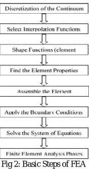
V. BASICSTEPSOFFEA

a)The given footing is divided into an equivalent system of finite elements, by a process known as Discritization. The equivalent system may consist of triangular or quadrilateral and/or tetrahedron or hexahedron based on whether the problem is solved as in 2-D or 3-D plane.

b)Once an element shape has been chosen, the analyst must determine how the variation of the field variable across the field domain is to be represented or approximated. In the most cases, a polynomial interpolation function is used.

c)The finite element method describes the behaviour of a continuum using a discretization of the continuum into smaller, manageable regions called elements. The unknown field variable or variables, (e.g. displacement) for which the solution is sought is expressed in terms of a discrete number of unknowns at each node

d)Once the interpolation functions have been chosen, the field variable in the domain of the element is approximated in terms of discrete values at the nodes. consequently, a system of equations is formed which expresses the element properties in terms of qualities at the nodes. For example, in a structural analysis, the element equations relate the nodal forces to the nodal displacements.

(3)

f)The global system of equations created in the previous step cannot be solved, pending application of the boundary conditions. Mathematically, before applying the boundary conditions, the system of equations is indeterminate and does not have a unique solution. In the same way that a structure must be physically fixed to the ground to prevent it from moving when a force is applied, a node must also be fixed to the ground.

g)Once the boundary condition has been applied to the assembly matrix of equations, standard numerical techniques can be used solve for the unknown field variable at each node.

h)In general, there are three phases in computer-aided engineering task;

i. Pre-processing: define the finite element model and environmental factors to apply to it. ii. Analysis: Solver-solution of finite element model.

iii. Post-processing of results using visualization tools.

Fig 2: Basic Steps of FEA

VI. BASIC STEPS TO SOLVE PROBLEM-USING MATLAB



Definition of Geometry:

The fig 3a shows a rectangular plate by 300mm X 300mm with 0.4 mm thickness and the elliptical cutout has been created in the plate with varying dimensions of major and minor axis.

(a) (b) (c)

Fig 3a) Geometry of FEA Model (b) Block diagram of FEA Model (c) Finding the corner data

The geometry has been divided into four equal parts.

 Identifying Block Corner and Midpoint Data:

Geometry has been divided in the previous step, it will arranged by order and obtain the XY Coordinates of each node. In order to determine the XY coordinates of the Circumference of the Elliptical geometry by using equation (2) (as shown in Fig 3 b & 3c)

+ = 1--- (2)

(4)

 Mesh Generation Program:

By using Finite Element Method, the program has been written to generate the mesh and the program is mentioned in Appendix-I

 Execution of the Mesh Generation Program:

After entering the corner data, midpoint data, we save this input file in the current directory side of MATLAB. Run the meshgen.m extension file. The command window will ask mesh gen input data file name. Enter<MESHGEN.INP>. Matlab command window will ask the name for an output file. Enter<MESHOUT.INP>. In order to obtain the mesh generation, number of nodes, number of elements we run <plot2d> file. Command window will ask again input data file. Enter <MESHOUT.INP>. Automatically mesh generated figure will appear in the figure window.

Fig 5: Mesh with Node and Element Numbering

In this figure5, there is no representation of number of nodes and elements. In order to see the mesh generation figure with node and element numbering we will enter 1, 2 and 3 respectively. (As shown in figure 5)

 To generate CST Input file by using MESH.GEN output file:

After completion of mesh generation stage, here we will determine the stresses in x-direction, y-direction and principal stress. The data’s like number of nodes, number of elements, displacement in x and y direction in each node and node numbering for each element are obtained in the <MESHOUT.INP> file. By using these data’s we will create a <CST.INP> file as shown below. In this <CST.INP> file we will add thickness (i.e., 0.4), temperature raise (negligible), young’s modulus (30e6) and poisson’s ratio (0.25). As per the boundary conditions we consider top most nodes as fixed. Since the nodes are fixed the displacement is zero. Here for each node there will two degrees of freedom in x and y direction respectively. [Program mentioned in Appendix –I ]

 Determination of Displacement, Reaction, Stress at each node

After generation of <CST.INP> file, we run the <cst.m> file in the command window. Then we go for plane stress analysis. The command window will ask input data file that is nothing but the <CST.INP> data file. Then it will ask output data file. Enter <CSTOUT.INP>. In this <CSTOUT.INP> file displacement at each node, reactions at constraints and stress at each element are obtained which are shown below fig 6.

(5)

Then the command window will ask to create a data file for Von-misses stress then we enter <estress.txt>. The displacement in x and y-direction for each node, reaction at the constraints in x and y-direction, maximum and minimum principal stresses for each element is displayed in the command window and as wellas it is saved in the <CSTOUT.INP> file.

VII. RESULT AND DISCUSSION

a) Plate with Elliptical Cutout when Minor Axis is Fixed:

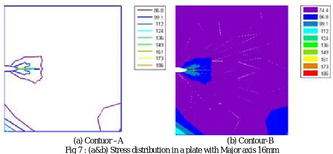
By fixing the minor axis as a 14mm and varying the major axis dimension like 16mm, 30mm, 45mm up to 105mm.Table 1 shows the readings for minor axis as 14mm, which is fixed and by varying the major axis throughout the analysis we take the thickness as 0.4mm which is negligible for 2D problems. Width of the plate is 150mm, which is fixed throughout the analysis. a/w ratio are determined for respective readings. Area is considered for a position in which load acts normally. With major axis as 16mm, we get maximum stress as shown in the Fig 7(a) and (b). By using this maximum stress we calculate numerical stress concentration factor. By comparing numerical stress concentration factor i.e. 3.99 with theoretical stress concentration factor i.e. 3.29 (by using theoretical relationship), we are near to the theoretical stress concentration factor. The error between theoretical and numerical stress concentration factor (kt) is 17.54%. From the table we came to know that stress is increases with increasing the size of the elliptical cutout. Hence the stress concentration is directly proportional to the major axis of the elliptical cutout. From this we came to know the thing is the stress concentration factor (kt) is directly proportional to the axis which is perpendicular to the load applied.

.

Table 1: Maximum stresses and Stress concentration Factor (Kt) with Minor axis 14mm

Minor axis, 2b (mm)

Major axis, 2a(mm

)

Width of plate, w (mm)

a/w ratio

Area, A=(w-a)t

( )

=

(N/ ) (N/ )

Numerical Kt

Theoretical Kt

14 16 150 0.1 53.6 46.64 186 3.99 3.29

14 30 150 0.2 48 52.08 309 5.93 5.29

14 45 150 0.3 42 59.52 493 8.28 7.43

14 60 150 0.4 36 69.44 848 12.21 9.57

14 75 150 0.5 30 83.33 1330 15.96 11.71

14 90 150 0.6 24 104.17 1950 18.7 13.86

14 105 150 0.7 18 138.88 3780 27.22 16

Table 1 shows the readings for minor axis as 14mm, which is fixed and by varying the major axis throughout the analysis we take the thickness as 0.4mm, which is negligible for 2D problems.

(a) Contuor –A (b) Contour-B Fig 7 : (a&b) Stress distribution in a plate with Major axis 16mm

(6)

Fig 8: Variation of Stress concentration factor with a/w ratio for Minor axis fixed (Numerical method)

The fig 7 (a) and (b) shows the maximum stress distribution in a plate in the form of contour A and contour B respectively. The fig 8 is represents the standard chart of the stress concentration factor (kt) verses major axis to width (a/w) ratio.

b) Plate with Elliptical Cutout when Major Axis is Fixed

Table 2 shows the readings for major axis as 94mm, which is fixed and by varying the minor axis throughout the analysis we take the thickness as 0.4mm which is negligible for 2D problems. With minor axis as 15mm, we get maximum stress as shown in the Fig 9 (a) &(b). By using this maximum stress we calculate numerical stress concentration factor (kt). By comparing numerical stress concentration factor i.e. 19.9 with theoretical stress concentration factor i.e. 13.53, we are near to the theoretical stress concentration factor. By comparing the theoretical result and numerical result we error around 32%. From these result we came to know that stress concentration value is inversely proportional to the minor axis of the elliptical cut-out. By increasing the value of the minor axis we can reduce the stress concentration value of the plate. Hence stress concentration factor (kt) is decreases with increasing the minor axis.

Table 2: Maximum stresses and Stress concentration Factor (Kt) with Major axis 94mm

Minor axis,

2b (mm)

Major axis, 2a(mm)

Width of plate, w (mm)

a/w ratio

Area, A=(w-a)t

( )

=

(N/ ) (N/ )

Numerical Kt

Theoretical Kt

15 94 150 0.1 22.4 111.6 2220 19.9 13.53

30 94 150 0.2 22.4 111.6 2120 18.99 7.27

45 94 150 0.3 22.4 111.6 1850 16.58 5.18

60 94 150 0.4 22.4 111.6 1630 14.6 4.13

75 94 150 0.5 22.4 111.6 1450 13 3.5

90 94 150 0.6 22.4 111.6 1190 10.66 3.1

Table 2 shows the readings for major axis as 94mm, which is fixed and by varying the minor axis throughout the analysis we take the thickness as 0.4mm which is negligible for 2D problems

(7)

With minor axis as 15mm, we get maximum stress as shown in the Fig 9 (a) &(b)

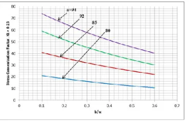
Fig 10: Variation of Stress concentration factor with b/w ratio for Major axis fixed (Numerical Method)

The Fig 10 represents the standard chart of the stress concentration factor (kt) verses minor axis to width (b/w) ratio. From this standard graph we can find out the stress concentration factor value for any given dimension of the elliptical cut out.

VIII.CONCLUSION

 The Plate with a dimension of 600mm X 300mm X 0.4mm and having an elliptical cut-out. For different major and minor axis along different values of Kt was obtained theoretically by using suitable formulas and keeping plate dimensions as a constant. Finite Element Method validated later theoretical calculation in numerical tool – MATLAB. The results were plotted on a graph taking a/w and b/w v/s stress concentration factor Kt. From the analytical result were compared with theoretical values.

 From the above analysis, we also came to know that stress concentration factor is directly proportional to the axis, which is perpendicular to the load applied. Hence stress concentration factor (kt) is directly proportional to the axis which is perpendicular to the load applied

REFERENCES

[1] Joseph E Shigley and Charles R Mischke, “Mechanical Engineering Design,” McGraw Hill International edition, 6th_{Edition 2003.}

[2] TirupathiR.Chandrupatla and Ashok D.Belegundu, “Introduction to Finite Elements in Engineering,” Third Edition, 2002.

[3] SingiresuS.Rao, “The Finite Element Method in Engineering,” BH Publication, 5th_Edition.

[4] V.B.Bhandari “Design of Machine Elements” 3rd edition Tata McGraw-Hill , PP: 141-150, 2010

(8)

Appendix I:

1. Mesh Generation Program:

Mesh Generation

Number of Nodes per Element <3 or 4> 3

BLOCK DATA

#S-Spans(NS) #W-Spans(NW) #PairsOfEdgesMergedNSJ)

1 4 0

SPAN DATA S-Span# Num-Divisions (for each S-Span/ Single division = 1) 1 4

W-Span# Num-Divisions (for each W-Span/ Single division = 1) 1 4

2 4

3 4

4 4

BLOCK MATERIAL DATA (for Material Number other than 1) Block# Material (Void => 0 Block# = 0 completes this data) 0 BLOCK CORNER DATA Corner# X-Coord Y-Coord (Corner# = 0 completes this data) 1 0 146

2 0 0

3 26.52 147.17 4 75 0

5 37.5 150

6 75 150

7 26.52 152.83 8 75 300

9 0 154

10 0 300

MID POINT DATA FOR CURVED OR GRADED SIDES S-Side# X-Coord Y-Coord (Side# = 0 completes this data) 0 W-Side# X-Coord Y-Coord (Side# = 0 completes this data) 1 14.35 146.3 3 34.65 148.47 5 34.65 151.53 7 14.35 153.69 | | | MERGING SIDES (Node1 is the lower number) Pair# Side1Node1 Side1Node2 Side2Node1 Side2node2 2. CST Input File: CST INPUT FILE NN NE NM NDIM NEN NDN 85 128 1 2 3 2 ND NL NMPC 10 5 0

Node# X Y

(9)

5 0.00000e+000 0.00000e+000 6 1.58750e+000 1.46079e+002 10 1.87500e+001 0.00000e+000 | | | | | | 71 3.06000e+000 1.53690e+002 72 1.16700e+001 1.90268e+002 73 2.02800e+001 2.26845e+002 74 2.88900e+001 2.63423e+002 84 0.00000e+000 2.63500e+002 85 0.00000e+000 3.00000e+002

Elem# N1 N2 N3 Mat# Thickness TempRise

1 1 2 7 1 .4 0

2 7 6 1 1 .4 0

3 2 3 8 1 .4 0

9 6 7 12 1 .4 0

10 12 11 6 1 .4 0

| | | | | | 21 13 14 18 1 .4 0

22 19 18 14 1 .4 0

29 18 19 23 1 .4 0

30 24 23 19 1 .4 0

| | | | | | 120 80 79 74 1 .4 0

121 76 77 82 1 .4 0