Use of Lagrange Multipliers to Provide an Approximate Method
for the Optimisation of a Shield Radius and Contents
Paul Warner1,* 1Rolls-Royce, Derby, UK
Abstract. For any appreciable radiation source, such as a nuclear reactor core or radiation physics accelerator, there will be the safety requirement to shield operators from the effects of the radiation from the source. Both the size and weight of the shield need to be minimised to reduce costs (and to increase the space available for the maintenance envelope on a plant). This needs to be balanced against legal radiation dose safety limits and the requirement to reduce the dose to operators As Low As Reasonably Practicable (ALARP). This paper describes a method that can be used, early in a shield design, to scope the design and provide a practical estimation of the size of the shield by optimising the shield internals. In particular, a theoretical model representative of a small reactor is used to demonstrate that the primary shielding radius, thickness of the primary shielding inner wall and the thicknesses of two steel inner walls, can be set using the Lagrange multiplier method with a constraint on the total flux on the outside of the shielding. The results from the optimisation are presented and an RZ finite element transport theory calculation is used to demonstrate that, using the optimised geometry, the constraint is achieved.
1 Introduction and Background
It is often required to design shielding around a radiation source in such a way that a radiation criterion is met on the outside of the shield. The shield itself may be composed of an array of different materials, each of which require optimisation in terms of thickness. A typical shield arrangement could be a steel water array composed of several steel shields placed at various distances from the source of radiation within a hydrogenous material. The question arises as to what is the overall radius of the shield and the optimum thicknesses of the steel shields given a constraint placed on the radiation level on the outside of the shield?
Although good neutron and gamma ray transport theory solvers are available to give predictions of the neutron flux or dose rate on the outside of a shield, the problem is still difficult since, if there are several shields to optimise, it is not clear how to decide on what the thickness of each shield should be. This is because the sensitivity of, for example, a steel shield in a water/steel array depends upon the distance from the source and also what steel shields are already included between it and a radiation source, such as a reactor core. In general, for this type of arrangement, the sensitivity of the dose rate on the outside of the shield is most sensitive to shields that are closest to the radiation source. This is due to the fact that, close to the reactor core, there will be a relatively high fast neutron population which is susceptible to inelastic scattering in steel. As this fast neutron population decreases by attenuation deeper into the shield, there will be relatively fewer fast neutrons and so this inelastic scattering process will be less efficient for outer steel shields. As a result, the outer steel shields become less effective.
The thicknesses of the shielding can be estimated by using a combination of engineering judgement and by running many design calculations using an appropriate neutron transport theory code to obtain an optimised design.
However, in order to reduce the number of calculations it would be better to have a more systematic way of performing the optimisation.
This paper describes an approximate method for undertaking such an optimisation based upon minimisation of a function using Lagrange multipliers. The overall method is described and then applied to a theoretical small reactor model which is surrounded by a primary shield composed of a steel water array.
2 Description of the Theory
Since the major constraint is that placed on the total neutron flux (or dose rate) on the outside of the primary shield, it is required to represent the flux as a mathematical function of all the required variables:
∅ = ( , ⋯ ) (1)
The first variable x1 is set equal to the shield radius. The other variables can be assigned arbitrarily. For example, x2 could be the inner Primary Shield Tank (PST) steel wall thickness and x3 could be a mid-wall and so forth.
The basic idea is to represent the change in flux on the outside of the PST by estimating the change as a function of radius assuming astarting guess. The otherparameters are then represented as variations to this:
∅ = ( ) + ( ) + ( ) ⋯ ( ) (2)
Where x1 is the radius of the shield and x2, x3 etc are the steel shield thicknesses.
() =
(3)
In order to supply constraints, a first order approximation is used by differentiating equation (1):
∅ =
+
+
+ ⋯
(4)
In equation (4) the partial derivatives are the sensitivity of the flux to a given parameter and can be labelled as Gi for convenience. Using the geometry from a transport theory calculation as the starting guess for the PST flux ∅, the variation in the flux, to first order accuracy, can be given by:
∅+ ∅ = ∅+ (− )
(5)
Where xs = 0 for i >1
If ϕ represents the user input constraint, eg the total neutron flux on the outside of the shield, then equations (2) and (5) may be combined using a Lagrange multiplier
λ to give a general function L of all the variables:
In the above equation, the coefficients a represent the quadratic coefficients where the range of i is from 1 to 3 and that for j ranges from 1 to N (where N is the number of parameters).
The optimized solution is obtained by partial differentiation of the function in equation (6) with respect to each variable and equating to zero. This yields a set of simultaneous equations which can be solved for each variable. The solutions are:
If = !" #"$%& '*- %.ℎ *' 0 1-2%!%-&
Let
4 = ∅5 − ∅+
6 = 724 +
9
(7)
The basic shielding parameters are then given by:
= 62−
'*- = 1, 0 (8)
The rest of the paper describes the theoretical shield model, the calculation of the required constants and sensitivities and the results from the optimisation method. The result of the optimisation is confirmed using a transport theory calculation and suggestions are given for future improvements to the method.
Description of the Shielding Problem
The method is generally applicable to most shielding problems where a radiation source requires a shield design. Examples include shielding a fixed source, accelerator shielding and reactor shielding.
It is required to reduce the geometry to a relatively simple form such that it can be represented by a 2D calculation. In principle the method can be applied to more complex geometries but this would have to be balanced against the number of calculations required to generate the sensitivity data.
A further limitation of the approach, is that it is not applicable to any shielding calculations where there exists significant streaming paths. Such streaming paths could create a significant bypass around the steel arrays considered in this paper and would therefore need to be treated separately.
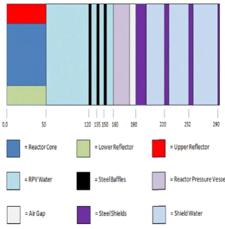
For this paper, a theoretical small reactor model was developed based upon a 235U fission source. A two dimensional RZ schematic diagram of the model is shown in Figure 1.
The model contains a representation of a central reactor core with a uniformly distributed 235U fission source equivalent to 500MW in strength. Outside the core, a number of typical steel components are modelled including steel baffles and a reactor pressure vessel. The shielding around the reactor is essentially a tank of water with a steel inner wall, two mid-wall shields and an outer steel shield.
Fig. 1 Schematic Diagram of the Shielding Problem (All dimensions in cm).
<(, , ⋯ ) =
− 6 >∅+ (− )
− ?5@
(6)
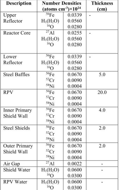
The material geometry information for the model is given in Table 1 along with the relevant material thicknesses.
Table 1. Material Geometry Data.
Description Number Densities
(atoms cm-3)×1024
Thickness (cm) Upper
Reflector
56Fe H1(H2O)
16O
0.0339 0.0560 0.0280
-Reactor Core 27Al
H1(H2O) 16O 0.0255 0.0560 0.0280 -Lower Reflector 56Fe H1(H2O)
16O
0.0339 0.0560 0.0280
-Steel Baffles 56Fe
52Cr 58Ni 0.0670 0.0090 0.0004 5.0
RPV 56Fe
52Cr 58Ni 0.0670 0.0090 0.0004 20.0 Inner Primary Shield Wall 56Fe 52Cr 58Ni 0.0670 0.0090 0.0004 4.0
Steel Shields 56Fe
52Cr 58Ni 0.0670 0.0090 0.0004 2.0 Outer Primary Shield Wall 56Fe 52Cr 58Ni 0.0670 0.0090 0.0004 2.0
Air Gap 27Al 0.0022
-Shield Water H1(H2O) 16O
0.0600 0.0300
-RPV Water H1(H2O)
16O
0.0600 0.0300
-A requirement was set to reduce the total neutron flux on the outside of the shield to fall just below 100 neutrons cm-2s-1. This value hence becomes the constraint for the Lagrange multiplier method. The method is then used to estimate the optimum thicknesses of the inner steel shield wall and also the two steel mid-walls shown in Figure 1.
4 Generating the Polynomial and Sensitivity
Data for the Lagrange Method
The Lagrange multiplier method as described in this paper requires a set of polynomials and sensitivities to be generated in order to represent the variation in neutron flux on the outside of the shield as a function of the variables that require optimising.
In order to calculate the neutron fluxes at the outer edge of the shield, a simple two dimensional RZ finite element transport theory calculation was used. The model shown schematically in Fig 1 was meshed using a two dimensional RZ mesh made up of rectangular finite
elements. The mesh contained 4408 elements and 4305 nodes. This mesh was input into the finite element even parity transport theory code EVENT [1]. The EVENT calculation was solved using a P7 order for the spherical harmonic expansion and a P3order for the scatter cross sections. The BUGLE96 library was used to provide the basic cross section data in 47 neutron energy groups.
Using the model shown in Fig1 as a starting point for the EVENT calculation, the total neutron flux summed over all 47 energy groups was calculated on the outside of the shield at the core centreline. The value produced by EVENT was 171 neutrons cm-2 s-1 which was used as the starting flux for the Lagrange multiplier method given in equation (5).
The next step was to change the radius of the shield and then recalculate the neutron flux on the outside of the shield. This was repeated for several shield radii to give the flux as a function of radius. A simple quadratic curve fit within EXCEL was used to provide the fitting coefficients as shown in Fig 2.
Fig. 2 Variation in Total Neutron Flux on the Outside of the Shield as a Function of Radius as Given by EVENT
Fig. 3 Variation in Total Neutron Flux on the Outside of the Shield as a Function of Inner Steel Wall Thickness
One of the approximations inherent in using this method is that the variation in the thickness in each shield is independent of the thickness of other shields. This could be overcome using more complicated fitting techniques but this would detract from the overall ease of use of the approximate optimisation method. In order to ensure that this was not entirely lost a conservative approach to the two mid-wall shields was used. In this case, the variation in flux with thickness of the first mid-wall was calculated using the thickest primary shield inner wall. Similarly, the variation in primary shield flux with second mid-wall thickness was generated with both the thickest inner wall and first mid-wall. The results are shown in Figures 4 and 5.
Fig. 4 Variation in Total Neutron Flux on the Outside of the Shield as a Function of First Steel Mid-Wall Thickness
Fig. 5 Variation in Total Neutron Flux on the Outside of the Shield as a Function of Second Steel Mid-Wall Thickness
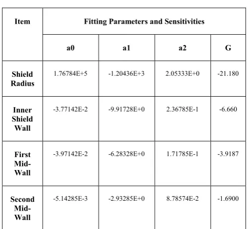
The sensitivities, G, in equation (5), are calculated by averaging the gradient of the respective plot over the range given in the figures. The quadratic fitting coefficients and the sensitivities are shown in Table 2.
Table 2. Fitting Parameters.
Item Fitting Parameters and Sensitivities
a0 a1 a2 G
Shield Radius
1.76784E+5 -1.20436E+3 2.05333E+0 -21.180
Inner Shield Wall
-3.77142E-2 -9.91728E+0 2.36785E-1 -6.660
First Mid-Wall
-3.97142E-2 -6.28328E+0 1.71785E-1 -3.9187
Second Mid-Wall
-5.14285E-3 -2.93285E+0 8.78574E-2 -1.6900
It is evident from Figure 2 that the variation in flux as a function of radius is not a good approximation for a first order sensitivity. As a result it was necessary to run through first iteration of the Lagrange method in order to get a realistic estimate of the shield radius. This first iteration was then used to derive the sensitivities that are given in Table 2. Once the polynomial coefficients and sensitivities are known then equations (7) and (8) can be readily solved to obtain the required estimates for the shielding parameters using the flux constraint of 100 neutrons cm-2 s-1.
As stated previously, applying the Lagrange method in the manner given above, gives a conservative result relative to the target flux of 100 neutrons cm-2 s-1. A small adjustment was thus made to the final shield radius using the sensitivity data to give the required target.
Discussion of Results
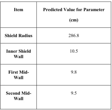
The result of the optimisation is given in Table 3.The shield radius and the predicted steel shield thicknesses were modelled in a P7 EVENT calculation (using a P3 order for the scatter cross-sections) in order to find out how close the method gets to the constraint. The EVENT result is shown in Table 4. As can be seen, the results from the Lagrange multiplier method agree well with that produced from EVENT(close to the theoretical estimate of 100 neutrons cm-2 s-1) while providing a reasonably practical optimisation of the shield thicknesses based upon the input sensitivities.
The results in Table 3 also show the expected behaviour in that the sensitivity to steel thickness increases as the shield is moved closer to the core. This is due to the effect caused by inelastic scattering of neutrons in steel which slows down fast neutrons to intermediate level. Once at theseenergies, the elastic scattering due to hydrogen in water becomes more important. The more steel placed between the core and the edge of the shield the less effective it becomes, since there will be fewer fast neutrons to slow down. The result is that the outer steel shields become increasingly less effective and hence the sensitivity of the flux on the outside of the shield becomes less. This is also shown in Figures 3 to 5. The effect in the Lagrange multiplier method is to make inner shields thicker than the outer shields. As can be seen the results exhibit this effect.
Table 3. Shield Parameters predicted by the Method
Item Predicted Value for Parameter
(cm)
Shield Radius 286.8
Inner Shield Wall
10.5
First Mid-Wall
9.8
Second Mid-Wall
9.5
Table 4. Comparison of the Estimated Fluxes using the Lagrange Fitting Parameters with an Event Calculation
Method Total Neutron Flux at the Edge of the Shield
(neutrons cm-2 s-1)
Lagrange Prediction 100
EVENT 90
Overall Conclusions and Future
Development
In this paper an approximate method has been described for the purpose of optimisation of a shield array of materials. The method, based upon Lagrange multipliers, has been shown to produce practical results for a theoretical reactor model surrounded by a steel water array. The method has been applied to the array and the results shown to agree with the validated transport theory code EVENT.
A major approximation used in the method is that of first order sensitivities. This has been shown to be mitigated by running an initial iteration of the algorithm in order to get close to the final shield radius. The sensitivities can then be re-calculated about the corrected radius and these can be used to improve the final results.
A second approximation associated with the method is that the sensitivities and fitting are calculated for each shielding parameter independently. This means that the interplay in the energy spectrum of the neutrons resulting from the variation in the thickness of the shields is not accurately modelled. The approach adopted in this paper was to calculate the sensitivity of each shield while the thickest previous shield was in place. This approach results in an overall conservative result with respect to any radiation criteria or constraint placed on the flux or dose rate on the outside of the shield. It is likely that as more shields are included in the array, this approximation may become too conservative and another approach may be required.
To overcome the aforementioned issue, a future improvement to the method would be to calculate several sets of sensitivities for two thicknesses of steel shields within the array corresponding to the thickest steel shield and also the thinnest. By iterating the method and using interpolation to the most appropriate value the method could be made more accurate. This would give a much more accurate estimate of the effect of energy spectrum on sensitivities for the appropriate shield thickness. The disadvantage of this approach is that twice as many transport theory calculations would be required to calculate the sensitivities.
6
Currently, it takes each EVENT calculation approximately 10 minutes on a single processor machine and a minimum of 3 calculations are required to fit the quadratic data for each shield. Hence, as the number of shields is increased it would mean doubling the number of transport theory calculations which may become impractical. This would need to be considered as part of a future study.
The method has not been applied to gamma ray transport. There is no reason why the method should not be successful for this case, but, often it is required to optimise a shield for both neutron and the gamma rays simultaneously. A future improvement would be to develop a fitting function based upon the sum of neutron and gamma dose rate on the outside of the shield. This would enable an approximate optimisation of a shield for both neutrons and capture gamma rays that result from neutron capture within the shield material.
Finally, it is intended to test the method more robustly in the future using a genetic algorithm in conjunction with a fast transport theory solver.