Concept of CFD model of natural draft wet-cooling tower flow
T. Hyhl´ık1,a
CTU in Prague, FME, Department of Fluid Dynamics and Thermodynamics, Technick´a 4, 166 07 Prague
Abstract. The article deals with the development of CFD model of natural draft wet-cooling tower flow. The physical phenomena taking place within a natural draft wet cooling tower are described by the system of conser-vation law equations along with additional equations. The heat and mass transfer in the counterflow wet-cooling tower fill are described by model [1] which is based on the system of ordinary differential equations. Utilization of model [1] of the fill allows us to apply commonly measured fill characteristics as shown by [2].The boundary value problem resulting from the fill model is solved separately. The system of conservation law equations is interlinked with the system of ordinary differential equations describing the phenomena occurring in the coun-terflow wet-cooling tower fill via heat and mass sources and via boundary conditions. The concept of numerical solution is presented for the quasi one dimensional model of natural draft wet-cooling tower flow. The simulation results are shown.
1 Introduction
Natural draft cooling towers are widely used in industry especially in large power plants and in chemical industry. Low efficiency of the cooling process of these towers will cause a loss of power generation or product quantity. Care-ful and accurate analyses of cooling towers can result in improvement of efficiency of cooling process.
The aim of cooling tower is to transfer waste heat from cooled water into the atmosphere. The air which is flowing through the cooling tower is warmed up and its humidity is increasing which leads to cooling of flowing water. The density of warmed air is decreasing unlike the surrounding air and this density difference produce the natural draft. Frequently encountered type of natural draft cooling tower is concrete structure of rotational hyperboloid shape. Typ-ical cooling tower of this kind can be larger then 100 m in height and diameter.
Cooled water is sprayed above the fill using the set of sprayers. In the channels of counterflow wet-cooling tower fill of film type water flows vertically down through the fill as a liquid film. Air is driven by a tower draft and flows vertically in the opposite direction. Heat and mass transfer occurs at the water and air interface. Evaporation and con-vective heat transfer cool the water, what leads to increase of air humidity and temperature. The water is leaving the fill and falling down in the form of rain. There is a pond in the bottom part of the cooling tower where water is col-lected.
The most intense heat and mass transfer occurs in the fill zone. The simplest model of heat and mass transfer in the fill is Merkel model [3] which is industry standard now. The more advanced models are e.g.. Poppe model [4] and model [1].
As an example of CFD models of natural draft cooling tower flow can be mentioned e.g. [5] and commercial code based [6].
a e-mail:[email protected]
2 Balance laws
The moist air flowing through the cooling tower will be considered as homogeneous mixture. The total value of ex-tensive quantityϕis expressed as
ϕ=
α
wαϕα, wα= ρρα,
α
wα=1, (1)
wherewαis the mass fraction of componentα. Local form
of the balance law is [7]
∂(ϕαρα)
∂t +
∂(ϕαραvk)
∂xk +
∂ϕαjkDα−jkα
∂xk −
σα=0. (2)
Diffusive flux density jk
Dα is expressed through the center
of mass velocity
vk=
α
wαvαk, (3)
jkDα=ρα(vαk−vk), (4)
where
α
jkDα=0. (5)
Diffusive flux jk
Dαcan be written using Fick’s law [8] as
jkDα =−Dα,m
∂ρα
∂xk
, (6)
whereDα,mis diffusion coefficient. Density of flux of
quan-tityϕwe express as
jk(ϕ)=
α
jkα(ϕα). (7)
Density of production ofϕis
σ(ϕ)=
α
σα(ϕα). (8)
Local form of balance law for quantityϕcan be written for the mixture as
∂(ρϕ) ∂t +
∂(ρϕvk)
∂xk −
∂jk(ϕ)
∂xk −
σ(ϕ)=0. (9) DOI: 10.1051/
C
Owned by the authors, published by EDP Sciences, 2014 /2 01
3 Moist air
The moist air is mixture of dry air and superheated or satu-rated steam. For a description of the cooling tower flow, let us consider the humid air as a mixture of dry air and water vapour. The liquid phase will be ignored in the model of moist air flow. The density of the moist air is
ρ=ρa+ρv, (10)
where the densities can be expressed using equation of state as
ρa=
paMa
RT , ρv= pvMv
RT . (11)
Mass fraction of dry air and mass fraction of water vapour we can express as
wa=
ρa
ρ, wv= ρv
ρ, (12)
where
wa+wv=1. (13)
Pressure can be expressed using Dalton’s law
p=pa+pv. (14)
Specific gas constant of mixture can be expressed by means of specific gas constants of both components
r=wara+wvrv. (15)
Specific heat capacity of the mixture is expressed as
cv=wacva+wvcvv. (16) Specific moisture indicates the weight of steam per kilo-gram of dry air
x= Vρv Vρa =
ρv
ρa =
pvMv
paMa
. (17)
Mass fractions can be expressed using specific moisture
wa=
1
1+x, wv= x
1+x. (18)
Equation of state of a mixture of dry air and water vapour is expressed using Dalton’s law, the definition of specific humidity and the definition of the overall density as
ρ= p RT
Ma(1+x)
1+Ma
Mvx
, (19)
whereMais molecular weight of dry air,Mvis molecular
weight of water vapour,Ris universal gas constant andTis temperature. Pressure can be expressed using the equation of state as
p= ρRT
1+Ma
Mvx
Ma(1+x) =
ρRT
Mv−wv(Mv−Ma)
MaMv
(20)
The total energy of moist air is expressed as the sum of internal energy and kinetic energy
e=u+vkvk
2 . (21)
In the case of moist air we are usually working with en-thalpy relative to one kilogram of dry air andxkilograms of water vapour
h1+x=cpata+x(l0+cpvta), (22) whereta = T −273.15 is temperature is degrees of
Cel-sius. In the case where we are working with enthalpy per kilogram of substance we can introduce
h=wacpata+wv(l0+cpvta). (23)
This definition of enthalpy is standard and is used when working with moist air, but due to the fact that the dry air and water vapour can be considered under atmospheric conditions as an ideal gases we can define ad hoc internal energy of unsaturated humid air as
u=(wacva+wvcvv)T =cvT. (24) The total energy of unsaturated moist air is expressed in the form
ρe=ρ cvT+vkvk
2
=ρ r κ−1T+
vkvk
2
, (25)
whereκis Poisson coefficient κ=cp
cv. (26)
4 Governing equations
Continuity equation for dry air can be written as
∂(ρa)
∂t + ∂(ρavk)
∂xk −
∂ ∂xk
Da,v∂ρ∂ a
xk
=0, (27)
whereDa,v is diffusion coefficient of dry air in the water
vapour. We can express the continuity equation of water vapour in the form
∂(ρv)
∂t + ∂(ρvvk)
∂xk −
∂ ∂xk
Dv,a
∂ρv
∂xk
=σv(xk,t), (28)
whereσv(xk,t) represents the density of source of water
vapour and diffusion coefficient of water vapour in the air isDv,a=Da,v. The system of momentum equations can be
written in the form
∂(ρvi)
∂t + ∂ ∂xk
ρv
ivk−σik=−ρgδi3−ζ(xk,t)ρ|
v|2
2 δi3, (29)
where−ρgδi3 represents the gravitational force acting on the flowing moist air,σikis the stress tensor in a flowing
fluid andζ represents a loss coefficient per meter. The en-ergy equation is written in the form
∂(ρe) ∂t +
∂ ∂xk
ρvke−σk jvj+q˙k
=σq(xk,t)−gρv3, (30)
whereσq(xk,t) is density of heat source where only
5 Quasi one-dimensional flow equations
The modification of governing equations for the case of quasi one-dimensional flow is performed for control vol-umeA(z)dz. Dry air continuity equation has form
∂(ρaA(z))
∂t +
∂(ρavA(z))
∂z =0. (31)
We include force acting on side wall−pdA(z) in the case of momentum equation. Finally we have the system of equa-tions for quasi one-dimensional flow of the form
∂(WA) ∂t +
∂(FA)
∂z =Q, (32)
where
W=
⎡ ⎢⎢⎢⎢⎢ ⎢⎢⎢⎢⎢ ⎢⎣
ρa
ρv
ρv ρe ⎤ ⎥⎥⎥⎥⎥ ⎥⎥⎥⎥⎥ ⎥⎦, F=
⎡ ⎢⎢⎢⎢⎢ ⎢⎢⎢⎢⎢ ⎢⎣
ρav
ρvv
ρv2+p v(ρe+p)
⎤ ⎥⎥⎥⎥⎥ ⎥⎥⎥⎥⎥
⎥⎦ (33)
and vector of sources is
Q=
⎡ ⎢⎢⎢⎢⎢ ⎢⎢⎢⎢⎢ ⎢⎢⎣
0 A(z)σv(z)
pdA
dz −A(z)(ρg+ζρ v2
2) A(z)(σq(z)+ρgv)
⎤ ⎥⎥⎥⎥⎥ ⎥⎥⎥⎥⎥
⎥⎥⎦. (34)
The system of governing equations can be modified by summing of individual continuity equations to get mixture continuity equation. The water vapour continuity equation is modified to get water vapour mass fraction equation.
W=
⎡ ⎢⎢⎢⎢⎢ ⎢⎢⎢⎢⎢ ⎢⎣
ρ ρv ρwv
ρe ⎤ ⎥⎥⎥⎥⎥ ⎥⎥⎥⎥⎥ ⎥⎦, F=
⎡ ⎢⎢⎢⎢⎢ ⎢⎢⎢⎢⎢ ⎢⎣
ρv ρv2+p
ρvwv
v(ρe+p) ⎤ ⎥⎥⎥⎥⎥ ⎥⎥⎥⎥⎥
⎥⎦ (35)
and modified vector of sources is
Q=
⎡ ⎢⎢⎢⎢⎢ ⎢⎢⎢⎢⎢ ⎢⎢⎣
A(z)σv(z)
pddAz −A(z)(ρg+ζρv22) A(z)σv(z)
A(z)(σq(z)+ρgv)
⎤ ⎥⎥⎥⎥⎥ ⎥⎥⎥⎥⎥
⎥⎥⎦. (36)
6 Computation of sources in fill zone
The system of governing equations is necessary to close. There are two unknown sources in the source vector (36), i.e. density of water vapour sourceσv(xk,t) and density of
heat sourceσq(xk,t). The sources in the fill zone can be
calculated using one dimensional model [1].
6.1 Balance laws
Due to the complexity of two phase flow occurring in the wet-cooling tower fill the one dimensional models of heat and mass transfer are used. These models are based on few assumptions which allow to create simplified one dimen-sional models. The first assumption talks about neglecting of the effects of horizontal temperature gradient in the liq-uid film, horizontal temperature gradient in air temperature
and humidity, see e.g. [4]. The second one states that tem-peratures and humidity are represented only by averaged value for each vertical position. We are also assuming that at the interface of two phases, there is a thin vapour film of saturated air at the water temperature, see e.g. [4].
The derivation of every one dimensional model of heat and mass transfer in the fill is based on balance laws. We have four variables in this problem:tatemperature of air,
twtemperature of water,xspecific humidity and ˙mwwater
mass flow rate. Mass balance of the incremental step of the fill is given by
d ˙mw+m˙adx=0, (37)
where ˙mais mass flow rate of dry air. The change in water
mass flow rate can be expressed using mass transfer coef-ficientαmas
d ˙mw=αm(x(tw)−x)dA, (38)
where x(tw) is saturated specific humidity at tw and dA
is infinitesimal contact area. The energy balance can be written in the form
˙
madh1+x=m˙wdhw+hwd ˙mw, (39)
whereh1+xis enthalpy of air water vapour mixture andhw
is enthalpy of water. The change in total enthalpy can be evaluated using interface parameters similarly like in the case of mass balance
˙
madh1+x=α(tw−ta)dA+hv(tw)d ˙mw, (40)
whereαis heat transfer coefficient and hv(tw) is enthalpy of water vapour.
6.2 Model of Klimanek & Białecky [1]
To derive the system of ordinary differential equations we have to choose independent variable. The model [1] is based on the selection of spatial coordinatezas independent vari-able contrary to Poppe’s model, see e.g. [4] which is based on the choice of water temperaturetw. The interface area
can be expressed using variablezas
dA=aqAf rdz, (41)
whereaqis the transfer area per unit volume andAf ris the
cross sectional area of the fill. We can derive equation for the change of the water mass flow rate from equation (38)
d ˙mw
dz =αmaqAf r(x
(tw)−x). (42)
To obtain the equation for the change of specific humidity in the fill we can substitute equation (42) into equation (37)
dx dz =
αmaqAf r(x(tw)−x)
˙ ma
. (43)
Differentiation of equation (22) leads to dh1+x
dz =(cpa+xcpv) dta
dz +(l0+cpvta)
dx
dz. (44)
after application of the definition of Lewis factor, which is equal to the ratio of heat transfer Stanton numberS tto the mass transfer Stanton numberS tm
Lef =
S t S tm =
α cpαm
, (45)
wherecpis constant pressure specific heat capacity of moist
air
cp=cpa+xcpv, (46) we can get
dta
dz =
αmaqAf r
˙
ma(cpa(ta)+x cpv(ta))
Lef(tw−ta)
cpa(ta)+ +x cpv(ta)
+(cpv(tw)tw−cpv(ta)ta)(x(tw)−x)
. (47)
By using equation (39) after substitution of equation (42) and equation (40) we derive equation for the change of wa-ter temperature
dtw
dz =
αmaqAf r
˙ mwcw(tw)
Lef(cpa(ta)+x cpv(ta))(tw−ta)+
+(x(tw)−x)(cpv(tw)tw−cpw(tw)tw+l0)
. (48)
The application of the Lewis factor in the previous equa-tions simplified the problem to find experimentally only mass transfer coefficientαmand calculate heat transfer
co-efficientαusing known value of Lewis factor. The most commonly used formula for the calculation of Lewis fac-tor is Bosnjakovic formula [9].
The driving force of evaporation process is (x(tw)−
x(ta))) in the case of supersaturation. The system of
or-dinary differential equations has to be changed [1]. The enthalpy of supersaturated air is
h1+x=cpata+x(ta)(l0+cpvta)+(x−x(ta))cw(ta)ta. (49)
Equations for the air and water temperature can be derived similarly like in the case of under-saturated moist air, see [1].
The system of four ordinary differential equations men-tioned in this section represents the boundary value prob-lem. We know air temperaturetaiand specific humidityxi
at air inlet and water temperaturetwiand water mass flow
rate ˙mion the opposite site of the fill because air and
wa-ter flows in the opposite direction. There is additional un-known set of parameters in the system of equations, i.e. αmaqAf r. These parameters have to be solved by using
ex-perimentally obtained characteristics of the fill [1, 2].
6.3 Fill zone simulation example
The calculation was performed for a fill of heightH=1 m. The air inlet mass flow rate is equal to ˙ma = 14333 kg/s
and water inlet mass flow rate is ˙mw = 17200 kg/s. Inlet
water temperature istwi = 34.9◦C. Air inlet temperature
istai = 15.7◦C and specific humidity at air inlet is xi =
7.622 g/kg. The atmospheric pressure is p = 98100 Pa. Outlet water temperature istwo=25.7◦C.
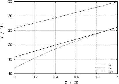
The numerical solution of the fill zone model was per-formed using Runge-Kutta method combined with shoot-ing method [2]. The calculated distributions of tempera-ture and humidity are depicted in figures 1 and 2. From the
10 15 20 25 30 35
0 0.2 0.4 0.6 0.8 1
z / m
t
/
◦C
ta
tw twb
Fig. 1.Distribution of air temperatureta, water temperaturetw and adiabatic saturation temperaturetwb
5 10 15 20 25 30 35 40
0 0.2 0.4 0.6 0.8 1
z / m
x
/
g
/
k
g
x x(t
a)
x(tw)
Fig. 2.Distribution of specific humidityx, saturation specific hu-midity at air temperaturex(ta) and saturation specific humidity
at water temperaturex(tw)
200 205 210 215 220 225 230 235
0 0.2 0.4 0.6 0.8 1
z / m
σv
A
/
k
g
/
s
/
m
Fig. 3.Distribution of density of mass source
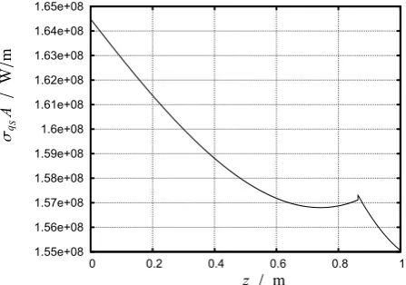
mentioned figures is possible to observe supersaturation in the upper part of of the fill, it means the air temperature is equal to adiabatic saturation temperature and specific humidity is slightly higher then saturation humidity. The distribution of the density of mass source is shown in the figure 3 and the density of sensible part of heat source is in the figure 4, where density of mass source of water vapour can be expressed as
σv= m˙a
A(z) dx
1.55e+08 1.56e+08 1.57e+08 1.58e+08 1.59e+08 1.6e+08 1.61e+08 1.62e+08 1.63e+08 1.64e+08 1.65e+08
0 0.2 0.4 0.6 0.8 1
z / m
σqS
A
/
W
/
m
Fig. 4.Density of sensible part of heat source distribution
and sensible part of heat source is
σqS = ˙ ma
A(z)
(dh1+x−l0dx)
dz . (51)
7 Cooling tower flow computation
Numerical solution is based on the (32), where because of the definition of total energy (25) the density of heat source should be calculated as
σq=σqS+273.15cpv(ta)σv (52)
7.1 Numerical method
The numerical solution utilizes cell-centered Finite Vol-ume Method in conservative form. Explicit MacCormack scheme is applied to solve system (32). Predictor step is expressed as
Win+1/2=Win−Δt μi
Fni+1Ai+1/2−FinAi−1/2
+ +Δμt
i
QiΔz
(53)
and corrector step is
Wn+1
i =
1 2
Win+Win+1/2−1 2
Δt μi
Fin+1/2Ai+1/2−
+Fni−+11/2Ai−1/2+ 1 2
Δt μi
QiΔz,
(54)
where
μi=Δz
Ai+1/2+Ai−1/2
2 . (55)
Jameson’s artificial diffusionAD(Wn i) [10] is
AD(Win)=CγWi−n1−2Win+Win+1, (56) where
γ= |pi−1−2pi+pi+1| |pi−1|+2|pi|+|pi+1|
. (57)
Vector of conservative variables is computed in new time level as
Win+1=Wn+1
i +AD(W
n
i). (58)
Total pressurep0and total temperatureT0are prescribed at the inlet boundary condition, where vector of conservative variables is calculated using extrapolated Mach number, see e.g. [11]. The outlet boundary condition is based on the prescription of static pressure and extrapolation of three components of the vector of conservative variables.
7.2 Calculation example
Natural draft cooling tower of rotational hyperboloid shape with
A(z)= π 4
0.006977z2−1.2764z+131.612 (59) is selected [12]. Tower height isHt=150mand fill zone is
placed at the height of 11.5m. Calculation was performed for fill heightH =1m. Water inlet mass flow rate is ˙mw=
17200 kg/s. Inlet water temperature istwi = 34.9◦C. Air
inlet temperature istai =15.7◦C and specific humidity at
air inlet is xi = 7.622 g/kg. The atmospheric pressure is
p =98100 Pa. Outlet water temperature istwo = 25.7◦C.
Prescribed parameters allows to quantify fill requirement to cool water fromtwi = 34.9◦C totwo = 25.7◦C. Outlet
static pressure in the heightHtis calculated using [13]
pout=p0
1−0.00975Ht T0
3.5(1+xi)(1−xi/(xi+0.62198)) . (60)
Total pressure at the tower inlet was recalculated using pre-vious equation to cooling tower inlet height 10m.
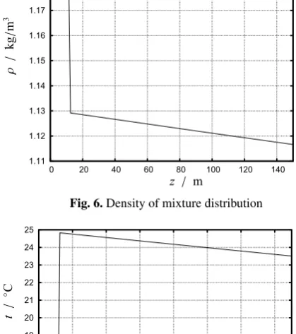
In figures 5, 6, 7, 8 and 9 the distribution of chosen parameters are shown over the tower height. The pressure decay in the figure 5 is affected not only by gravity but also by losses in the rain and fill zones. There is a drop in the density distribution in the figure 6 which is connected with heat addition in the fill zone. The heat addition is af-fecting also the distribution of temperature in the figure 7 where the sharp increase of temperature in the fill zone is observed. The mass source in the fill zone leads to jump in the distribution of specific humidity as shown in the figure 8. The decrease of temperature and humidity in the upper part of the cooling tower is natural and is connected with gravitational force acting on flowing moist air. The effect of heat addition in the fill zone is perceptible also in the distribution of velocity. There is slight increase of velocity in the fill zone, see figure 9. The increase of velocity in fill zone have to compensate the mentioned drop in the density distribution.
8 Conclusions
96200 96400 96600 96800 97000 97200 97400 97600 97800 98000
0 20 40 60 80 100 120 140
z / m
p
/
Pa
Fig. 5.Static pressure distribution
and rain zone, where additional heat and mass transfer oc-curs. Last but not least it is necessary to mention the limit of one dimensional approach. Author is going to overcome imperfections and limits of this model in future work.
9 Acknowledgement
This work has been supported byTechnology Agency of the Czech Republicunder the projectAdvanced Technologies for Heat and Electricity Production - TE01020036.
References
1. A. Klimanek, R. A. Białecky, International Communi-cations in Heat and Mass Transfer36, (2009), 547-553 2. T. Hyhl´ık,Engineering Mechanics 2013,19th
Interna-tional conference, Svratka, (2013)
3. F. Merkel, Verdunstungsk¨uhlung, VDI Forschungsar-beiten, no. 275, VDI - Verlag, Berlin, 1925
4. N. J. Williamson, Numerical Modelling of Heat and Mass Transfer and Optimisation of a Natural Draft Wet Cooling Tower.Ph.D. thesis, University of Sydney, 2008 5. A. K. Majumdar, A. K. Singhal, D. B. Spalding, ASME
J. Heat Transfer,105(4), (1983)
6. N. Williamson, M. Behnia, S. Armfield, Int. Journal of Heat and Mass Transfer,51(2008)
7. F. Marˇs´ık,Flow of Heterogeneous Mixtures with Relax-ation Processes(in czech), Institute of Thermomechan-ics, Academy of Sciences of the Czech Republic, Prague, 1994
8. A. Bejan, Convection Heat Transfer, John Wiley & Sons, 2004
9. F. Bosnjakovic, P. L. Blackshear Jr. (Ed.), Techni-cal Thermodynamics, Holt, Rinehart and Winston, New York, 1965
10. P. Punˇcoch´aˇrov´a-Poˇr´ızkov´a, K. Kozel, J. Hor´aˇcek, J. F¨urst, Engineering Mechanics,17(2), (2010)
11. J. Halama, F. Benkhaldoun, J. Foˇrt, Int. Journal for Numerical Methods in Fluids,65(8), (2011)
12. I. Z´u˜niga-Gonz´alez,Modelling Heat and Mass Trans-fer in Cooling Towers with Natural Convection. Ph.D. thesis, Czech Technical University in Prague, 2005 13. D. G. Kr¨oger,Air-Cooled Heat Exchangers and
Cool-ing Towers.Penn Well Corporation, Tulsa, 2004
1.11 1.12 1.13 1.14 1.15 1.16 1.17 1.18
0 20 40 60 80 100 120 140
z / m
ρ/
k
g
/
m
3
Fig. 6.Density of mixture distribution
15 16 17 18 19 20 21 22 23 24 25
0 20 40 60 80 100 120 140
z / m
t
/
◦C
Fig. 7.Distribution of temperature
6 8 10 12 14 16 18 20 22
0 20 40 60 80 100 120 140
z / m
x
/
g
/
k
g
Fig. 8.Distribution of specific humidity
1 1.5 2 2.5 3 3.5
0 20 40 60 80 100 120 140
z / m
v/
m
/
s