Distributed orbit determination for Global

Article

1

Distributed orbit determination for Global

2

Navigation Satellite System with inter-satellite link

3

Yuanlan Wen 1_{*, Jun Zhu} 2_{, Youxing Gong} 3_{, Qian Wang}1_{, Xiufeng He} 1,_*

4

1 _{School of Earth Sciences and Engineering, Hohai University, Nanjing 210098, China;}

5

[email protected](Y.W.); [email protected](Q.W.); [email protected](X.H)

6

2 _{Xi’an Satellite Control Center, Xi’an 710043, China; [email protected] (J.Z)}

7

3 _{Undergraduate School, National University of Defense Technology, Changsha 410073, China;}

8

[email protected](Y.G)

9

* Correspondence: [email protected]; [email protected]; Tel.: +86-25-83786961

10

11

12

Abstract: To keep the global navigation satellite system functional during extreme conditions, it

13

is a trend to employ autonomous navigation technology with inter-satellite link. As in the newly

14

built BeiDou system (BDS-3) equipped with Ka-band inter-satellite links, every individual

15

satellite has the ability of communicating and measuring distances among each other. The system

16

also has less dependence on the ground stations and improved navigation performance. Because

17

of the huge amount of measurement data, centralized data processing algorithm for orbit

18

determination is suggested to be replaced by a distributed one in which each satellite in the

19

constellation is required to finish a partial computation task. In current paper, the balanced

20

extended Kalman filter algorithm for distributed orbit determination is proposed and compared

21

with whole-constellation centralized extended Kalman filter, iterative cascade extended Kalman

22

filter, and increasing measurement covariance extended Kalman filter. The proposed method

23

demands a lower computation power however yields results with a relatively good accuracy.

24

Keywords: Inter-satellite link; Whole-constellation centralized extended Kalman filter;

25

Distributed orbit determination; Iterative cascade extended Kalman filter; Increased

26

measurement covariance extended Kalman filter; Balanced extended Kalman filter

27

28

1. Introduction

29

For global navigation satellite system (GNSS),currently, the master control station (MCS)

30

collects the satellite to monitor station measurement data, estimates the satellite ephemeris and clock

31

offsets, and generates a time stream of navigation messages. The messages are then uploaded to

32

satellites by ground antennas to broadcast to the user community [1]. However, the MCS as well as

33

the other ground-based segments including monitor stations and ground antennas have the risk of

34

destruction during a warfare or natural disaster. This is the case especially for the monitor stations

35

which distributed globally for increasing the accuracy of satellite orbit determination [2]. In order to

36

enhance the viability of the satellite navigation systems under the potentially fatal conditions, as early

37

as in 1980s, the autonomous navigation techniques using inter-satellite link (ISL) measurements

38

without supports from the MCS were investigated for the global positioning system (GPS) [3]. If the

39

ISL measurement was the unique source for orbit determination and time synchronization, the datum

40

mark would be insufficient [4]. This problem can be addressed by setting up a few ground anchorage

41

stations (GASs) which provide reference coordinate system and time system [5]. Combining both the

42

ISL and satellite-to-GAS measurements, the autonomous navigation system has several features:

43

firstly, the data processing will be completed by satellite onboard computers rather than the MCS;

44

secondly, the GASs can be considered as pseudo-satellites; and finally, the globally allocated monitor

45

stations can be replaced by a few domestic GASs [3].

46

Centralized data processing technique, which is widely applied in current autonomous

47

navigation constellation, collects the ISL and satellite-to-GAS measurement data, combines all the

48

satellite state vectors (including satellite orbit, clock error parameters, etc.) into one matrix, and

49

computes the optimal state vector for each satellite by a central satellite on-board computer. As

50

results, the associated state vector covariance matrix could be very large, the method requires a vast

51

computation power [6]. It is worth to mention that, in this case, every satellite is observed indirectly

52

by other satellites.

53

Whereas in distributed data processing algorithm, the computation is broken down and assigned

54

to each satellite. Each satellite is required to deal with self-related ISL measurements and local state

55

vectors. In this way, the number of measurement equations and dimension of the state vectors are

56

reduced. As a result, the computational amount of the whole system are decreased considerably.

57

Moreover, the accuracy of the orbit ephemeris and clock offsets calculated by distributed data

58

processing method could have the same level to the results of centralized data processing.

59

With the measurements from ISLs and satellite-to-GASs, the autonomous navigation

60

constellation constitutes an extremely complex system. Each satellite has to finish the task of ISL

61

measurement, data processing, and communicating. A practical algorithm for autonomous orbit

62

determination is still under development. Based on the method of iterative cascade extended Kalman

63

filter (ICEKF) and increased measurement covariance extended Kalman filter (IMCEKF), a new

64

distributed method, balanced extended Kalman filter (BEKF), is proposed in this paper. Together

65

with whole-constellation centralized extended Kalman filter (WCCEFK), four different autonomous

66

navigation algorithms are conducted in simulations for comparisons of accuracy and computation

67

loads.

68

2. Overview of Orbit Determination Algorithms

69

Ananda [7] proposed the framework of autonomous navigation system without a MCS at the

70

first time and validated the system by simulations. Rajan [3] introduced various autonomous

71

navigation algorithms and presented preliminary on-orbit experiment results.

72

In the designing of the GPS Block IIR, the ISLs, programmable microprocessors, and redundant

73

management were carried out. The following two major features are critical to ensure high precision

74

autonomous navigation [3, 7]:

75

 The ISL communications and measurements in UHF band.

76

 A high-precision autonomous navigation algorithm which is adapted to the computing

77

capacity of the satellite on-board computers;

78

A time division multiple access (TDMA) system, which has two frames, was employed for

79

ranging and data transmission. In ranging frame, each satellite is assigned a 1.5-second slot to make

80

pseudo-range (PR) measurements with the visible satellites. Two frequencies were used in the

81

measurement for ionospheric delay corrections. In data frame, a 1.5-second slot was appointed to

82

each satellite to transmit data includes the PR measurements, the estimated satellite state vector, and

83

the associated covariance matrix to all visible satellites.

84

The GPS Block IIF follows the design of the GPS Block IIR and improves the performance of ISL

85

measurements and on-board data processing. Without contacting with the ground system, Block IIF

86

can operate about 60 days in the autonomous navigation mode and provide navigation messages

87

which are corrected by ISL measurements with a 3-meter user range error (URE) (URE is a root mean

88

square value and does not consider the impact of the polar motion and UT1). However, it is difficult

89

to establish a precise prediction system because of the irregular polar motion and uncertain UT1.

90

Therefore, in autonomous navigation mode, the URE is far greater than 3 meters in a 60-day duration

91

[8].

92

For the GPS III, each satellite in the constellation will have the ability of ISL measurements and

93

communications. It is designed that once there are enough number of satellites in orbit, the GPS

94

constellation will be able to operate autonomously in wartime, but currently they are still under

95

investigation [9].

Galileo navigation system is also planned to employ autonomous navigation algorithm based

97

on ISLs [10]. Spatial orientation problem is solved by the combination of the ISL and

satellite-to-98

ground measurements. The simulation for Galileo system showed that URE is on the level of

99

decimeters [10], which is better than that of GPS.

100

For the distributed navigation algorithms, several techniques including iterative cascade

101

extended Kalman filter (ICEKF), increased measurement covariance EKF (IMCEKF), and

Schmidt-102

Kalman Filter (SKF) are discussed by Schmidt, Park and Ferguson [11-13]. The ICEKF is employed to

103

processes a large number of space-borne GPS measurement data and a small quantity of ISL

104

measurement data for low-Earth orbit formation flying satellites. In this method, the computation

105

process will iterate for 3 to 4 times for convergence and a good orbit accuracy is presented. For the

106

method of IMCEKF, amendments are made based on ICEKF and it presents a better performance. On

107

the other hand, the SKF yield results with a less accuracy compared to IMCEKF while processing the

108

GNSS ISL measurement data [4]. Recently, International Association of Geodesy (IAG) initiates a GPS

109

Dancer project which develops a distributed data processing algorithm to analyze the precision of

110

the GPS [14].

111

In China, distributed orbit determination and time synchronization algorithms based on ISL

112

measurements were studied [15-21]. The distributed autonomous ephemeris updating were

113

discussed for navigation satellites [22]. There are also many researches on developing higher

114

precision orbit determination methods for new BeiDou (BDS-3) experimental satellites in the

115

literature [23-26]. Currently, the developments for autonomous orbit determination, time

116

synchronization, and autonomous operation and management are wildly investigated. More

117

progress on designing an efficient distributed data processing algorithm, however, needs to be made.

118

3. Fundamental Equations for Measurement and Motion

119

3.1. Equations for Measurement

120

The position vectors,

r



i

=

[

x

i

y

i

z

i

]

T, velocity vectors,

v



i

=

[

v

_xi

v

i_y

v

i_z

]

T, and dynamic

121

parameter vector,

x

i_D

,

consititue the state vector which need to be estimated:

122

T i iT iT i T

D

v

x





=

_

 

_

X

r

(1)

123

In here, the superscript, T, denotes the transpose of a matrix, and the superscript, i, denotes that it is

124

for the ith _{satellite. The reference values for the state vector are stored in}

X

i*_{, and the improving}

125

values for the state vector are written in:

126

*

i i i

δ

x = X

−

X

(2)

127

After correcting the hardware delay, ionospheric delay, relativistic effect, multi-path effect, and

128

the antenna phase center offset [4], two one-way ISL PRs between the ith _{satellite and j}th _{satellite need}

129

to be translated into a same measurement epoch (e.g. ranging frame epoch t). The PR equations are:

130

( )

[

( )

( )]

(

( ),

( ))

( )

i j

_t

_c

_{t t}

j

_{t t}

i

_d

j

_t

i

_t

i j

_t

ρ

→

_{= ⋅ δ}

_{− δ}

₊

_X

_X

₊

ε

→

(3)

131

( )

[

( )

( )]

(

( ),

( ))

( )

j i

_t

_c

_{t t}

i

_{t t}

j

_d

j

_t

i

_t

j i

_t

ρ

→

_{= ⋅ δ}

_{− δ}

₊

_X

_X

₊

ε

→ ₍₄₎

132

where, c is the speed of light,

δ

t t

i

( )

and

δ

t t

j

( )

are clock errors for the ith _{satellite and the j}th _satellite,

133

( )

i j

_t

ε

→ _and

_ε

j i→

_{( )}

_t

_{are the measurement errors,}

_d

₍

_X

j

_{( ),}

_t

_X

i

_{( ))}

_t

₌

134

2 2 2

( i j) ( i j) ( i j)

x −x + y −y + z −z is the geometric distance between the two satellites.

135

Combining equations (3) and (4), distance measurement equation that only contains orbit parameter

136

is derived as:

( )

( )

( ) 2

(

( ),

( ))

( )

ij

_t

j i

_t

i j

_t

_d

j

_t

j

_t

ij

_t

ρ

₌

_

ρ

→

₊

ρ

→

_

₌

₊

ε





X

X

(5)

138

where,

ε

ij

( ) [

t

_k

=

ε

i→j

( )

t

_k

+

ε

j i→

( )] / 2

t

_k . Subtracting equation (4) from equation (3), time

139

measurement equation that only contains clock error parameters is deduced as:

140

( )

( )

( ) 2

[

( )

( )]

( )

( ) 2

ij j i i j j i j i i j

clock

t

t

t

c

t t

t t

t

t

ρ

₌

_

ρ

→

₋

ρ

→

_

_{= ⋅ δ}

_{− δ}

₊

_

ε

→

₋

ε

→

_









(6)

141

Following the steps above, the distance measurements and the clock bias measurements are

142

decoupled, the orbit ephemeris and clock offsets can therefore be estimated independently.

143

Linearizing equation (5) with Taylor expansion at the reference state vector

X

i*and

X

j* yields:

144

(

)

* *

* *

( )

( )

( )

,

( )

j i

ij ij

ij i j i j ij

i j

t

t

t

d

ρ

x

ρ

x

t

ρ

=

+

δ

+

δ

+ +

ε

∂

_X

∂

_X



X X

X

X

(7)

145

After that, equation (7) is converted into a linear measurement equation:

146

( )

( )

( )

( )

ij i i j j ij

z t

=

H x

_δ

t

+

H x

_δ

t

+

_ε

t

(8)

147

where

_{z t}

ij

( )

₌

_ρ

ij

( )

_t

₋

_d

(

_X

i*

,

_X

j*

)

is the innovation,

H

i and

H

j are the measurement

148

matrices.

149

(

) (

) (

)

*

*

* * * * * *

( )

,

,

,

i

i

ij i j i j i j

i

i i j i j i j

t

x

x

y

y

z

z

H

d

d

d

ρ



_

−

−

−



_

=

=

∂

X

X



_

X

X

X

X

X

X



_

_X

(9)

150

*

( )

-j ij

j i

j

t

H

=

ρ

=

H

∂

X

_X (10)

151

Similarly, GAS can be considered as a pseudo-satellite. The PR needs to be corrected by an extra

152

tropospheric delay compared to a normal satellite. Distance measurement equation that contains

153

orbit parameters between gth _{GAS and i}th _{satellite is derived as}

154

( )

( )

( ) 2

(

( ),

( ))

( )

ig

_t

g i

_t

i g

_t

_d

i

_t

g

_t

ig

_t

ρ

₌

_

ρ

→

₊

ρ

→

_

₌

₊

ε





X

X

(11)

155

In the equation (11) , the array of state parameters of GAS

X

g

( )

t

is known, only the state vector

156

of ith _{satellite is unknown. The reference ground coordinate is hence introduced into the satellite state}

157

by equation (11), this overcomes the lack of the datum mark in data processing while only ISL

158

measurements are utilized. The current linearized measurement equation which is similar to

159

equation (8) becomes:

160

( )

( )

( )

ig i i ig

z t

=

H x

_δ

t

+

_ε

t

(12)

161

3.2. Equations for Motion

162

Satellites can be affected by a variety of factors when operated in orbit. For navigation satellites

163

in here, only the gravitational forces, solar radiation pressure, and relativistic effects are considered

164

[27]. The gravitational forces include the attractions from the earth, the moon, and other planets in

165

the solar system. The dynamic equation for the ith _{satellite can be written as:}

166

c

( )

(

,

)

i

_t

₌

_f

i i



X

X w

(13)

where

f

c is a continuous function,

w

iis the system disturbances that has the following properties:

168

T

( )

( )

0,

( )( ( ))

0

i

i i i

t

t

E

t

E

t

t

τ

τ

τ



₌





₌





₌

_









_≠



Q

w

w

w

(14)

169

[ ]

E

⋅

denotes the expected value and

Q

i

( )

t

is a covariance matrix which is symmetric, non-negative,

170

and definite. In here, the system disturbances are simulated by Gaussian white noise. Because the

171

continuous function

f

c and the system disturbance

w

iis not coupled with each other, Equation (13)

172

can be written as:

173

c

( )

(

( ))

i

_t

₌

i

_t

₊

i



X



X

Gw

(15)

174

in which G =

[

0 I 0

]

T is coefficient matrix, and the

I

is the identity matrix, the 0 is the zero

175

matrix. Equation (15) is then linearized by Taylor expansion at the reference state vector

X

i* as:

176

*

c

c *

(

)

*

( )

(

( ))

(

( )

( ))

i i

i i i i i

i

t

₌

t

₊

∂

t

₋

t

_{+ +}

∂



_

X

X

X

X

X

X

Gw

X





(16)

177

From equation above, the state increments are then derived as:

178

( )

( )

( )

i

_t

_t

i

_t

i

δ

x



=

F

δ

x

+

Gw

(17)

179

where

δ =

x



X



−



c

(

X

i*

( ))

t

and

F

( )

t

is the dynamic partial derivative matrix[6]:

180

*

*

c c c c

D

|

0

0

( )

( )

0

0

t









∂

_

∂

∂

∂

_

=

_

_

∂

∂

∂

∂











=

X

X

I

X

F

X

r

r

p

0









(18)

181

The equation (17) is the state equation of the stochastic linear continuous systems and its general

182

solution is:

183

0

0 0

( )

( , )

( )

t

( , ) ( )d

i i i i i

t

t

t t

t

t

_τ

_{τ τ}

δ

x

=

Φ

δ

x

+

G



Φ

w

(19)

184

in which,

Φ

i

( , )

t t

₀ is the system state transition matrix and is the solution of the following equations:

185

0 0 0 0

( , )

( )

( , ),

( , )

i

_{t t}

₌

_t

i

_{t t}

i

_{t t}

₌



Φ

F

Φ

Φ

I

₍₂₀₎

186

where

I

is the identity matrix with the same dimensions as dynamics matrix,

F

( )

t

.

187

The state transition matrix

Φ

i

( , )

t t

₀ has the following features:

188

1

0 0

( , )

( , )

( , ),

( , )

( , )

i

_t

_τ

i

_τ

_t

₌

i

_{t t}

_

i

_t

_τ

_

−

₌

i

_τ

_t





Φ

Φ

Φ

Φ

Φ

(21)

189

In the actual computation process, discretization needs to be implemented for equation (19):

190

1

1 1 1

( ,

)

k

( , )

( )d

k t

i i i i i

k

t t

k k k _t

t

k

τ

k

τ τ

−

− − −

δ =

x

Φ

δ

x

+

G



Φ

w

(22)

191

In a sampling interval from

t

_k−1 to

t

_k, the white noise

w

i_k−1

( )

τ

can be considered as a constant.

192

The integral coefficient denotes that:

193

1

=

k

( , )d

k t i

k _t

t

k

τ τ

−



G G

Φ

(23)

For simplicity, the white noise will be denoted as 1 i k−

w

in the following paper. Then the

195

discretized state equation derived from equation (22) is:

196

1 1 1

i i i i i

k k− k− k k−

δ =

x

Φ

δ

x

+

G w

₍₂₄₎

197

In which,

Φ

_k−i ₁denotes the state transition matrix from

t

_k−1 to

t

_k. According to equation (24), the

198

predicted state covariance matrix is

199

i T i T 1

ˆ

1 1 1 1 1

i i i i i

k

=

k− k− k−

+

k− k− k−

P

Φ

P

Φ

G Q G

₍₂₅₎

200

4. Whole-Constellation Centralized Extended Kalman Filter

201

The whole-constellation centralized extended Kalman filter (WCCEKF) is one of the centralized

202

data processing method. According to this method, a main satellite and a back-up satellite are

203

assigned to complete the task of data processing. The other satellites in the constellation need to send

204

their measurement data, state vectors and corresponding covariance matrices to the main satellite for

205

orbit determinations.

206

For all the satellites in the constellation, the states and corresponding improving values from

207

equations (1) and (2) are collected and stored in a state vector

X

_kand an improving values vector

208

k

δ

x

[6, 28]

:

209

T

1T 2 T i T n T

k

=

（ ） （ ）







（ ）



（ ）





X

X

X

X

X

(26)

210

T

1 T 2 T i T n T

k k k k k

δ

_x

₌

（

_



δ

_x

） （

δ

_x

）



（

δ

_x

）



（

δ

_x

）

_



₍₂₇₎

211

where n is the number of satellites in the system. In this way, the state equation for all the satellites

212

can be obtained through Equation (24):

213

1 1 1

k k− k− k k−

δ =

x

Φ

δ

x

+

G w

₍₂₈₎

214

State transition matrix

Φ

_k and integral coefficient matrix

G

_k are diagonal matrices and can be

215

expressed as:

216

1 2

1 1 1 1 1

i n

k− =diagonal（ k−）（ k−）  （ k−）  （ k−）

Φ Φ Φ Φ Φ (29)

217

1 2 i n T

k =diagonal（ k）（ k）  （ k）  （ k）

G G G G G (30)

218

State noise vector,

w

_k−1

, stores the noise for

all the satellites in the constellation:

219

T

1 2

1 1 1 1 1

i n

k k k k k

w

₋

=

（



_

w

₋

）（

w

₋

）



（

w

₋

）



（

w

₋

）

_



(31)

220

and it has the statistical characteristics as follows:

221

1 1 0, 1( 1)

0

i

i j T k

k k k

i j

E E

i j

− − − −

 ₌

 ₌  _=

    _≠



Q

w w w (32)

222

1 2

1 1 1 1 1 1 1

T i n

k k k k k k k

E_w w_{− − }=Q ₋ =diagonal_Q ₋ Q ₋  Q ₋  Q ₋ _ (33)

223

The measurement equation which is a combination of equations (8) and (12) is then derived as:

224

k k k

z

=

H x +

δ

ε

(34)

225

where

H =

_k

[

0



(

H

i

)

T

 

0

(

H

j

)

T



0

]

T,

z

_k

=

z t

ij_k

( )

_k ,

ε

_k

=

ε

ij

( )

t

_k for ith _{satellite and j}th

226

satellite with ISL;

H =

_k

[0



(

H

i

)

T



0]

T,

z

_k

=

z t

_kig

( )

_k ,

ε

_k

=

ε

ig

( )

t

_k for GAS to ith _satellite

measurement. Next, a measurement covariance matrix

R

k

=

E(

ε ε

k kT

)

,

an initial state vector

228

* 0

=

E(

0

)

X

X

and an initial state vector covariance

P

0

=

E[

X X

0* 0*T

]

are defined. Finally, the method

229

of WCCEKF that combines the satellite-to-satellite measurements and satellite-to-GAS

230

measurements can be expressed as [29]:

231

T T

1

ˆ

1 1 1 1 1 k

=

k− k− k−

+

k− k− k−

P

_Φ

P

_Φ

G Q G

₍₃₅₎

232

(

)

1 T T

k k k k k k k

−

=

+

K

P H H P H

R

(36)

233

ˆ

_{k k k}

x

z

δ

=

K

(37)

234

ˆ

X

_k

=

X

_k

+

δ

x

ˆ

_k

X

ˆ

_k

=

X

_k

+

δ

x

ˆ

_k

(38)

235

(

)

ˆ

k

=

−

k k k

P

I K H P

(39)

236

The dimension of state vector

X

_kis

237

1

6 n i

W

i

N n D

=

= +

å

(40)

238

where Diis the number of dynamic parameters for the ith _satellite.

239

In the method of WCCEKF, each satellite is correlated with the other satellites through the state

240

vector covariance matrix which has the dimension of

N

_W

´

N

_W . What is more, matrix

241

T

(

H P H

_{k k k}

₊

R

_k

)

with the dimension of

m m

´

(

m

is the dimension of the measurement vector)

242

needs to be inversed during the process and a huge computational amount is expected. The

243

computation amount for a process of WCCEKF is:

244

2 2

4

N

_W

(

N

_W

_{− +}

1) (

N

_W

₋

1)

N

_W

(

N

_W

₊

1) / 6

+

₍₂

2

₊₇

₁₎

W W

N

N

_{+ ×}

m

(41)

245

If the WCCEKF algorithm is employed, the on-board computer of the main satellite would need

246

to process all the ISL measurement and satellite-to-GAS measurement data to finish the task of orbit

247

determination and navigation message generation for satellites in the constellation. Due to the huge

248

computation amount and great complexity of communication, WCCEKF is difficult to be

249

implemented in a satellite constellation with limited on-board computation ability.

250

In addition, the WCCEKF is also vulnerable. Once the main satellite and its backup satellite

251

failed, the entire navigation constellation would stop working. To avoid the drawbacks in the

252

WCCEKF method, many researches nowadays are focusing on developing the distributed data

253

processing algorithm.

254

5. Distributed Orbit Determination

255

For the distributed orbit determination algorithms based on the ISL, data processing is assigned

256

to each satellite. In this process, each satellite collects the ISLs measurement data with respect to its

257

visible satellite and estimates the self-related state vectors.

258

5.1. Reduced-Order Iterative Cascade EKF

For ith _{and j}th _{satellites with ISL measurements, the iterative cascade EKF (ICEKF) [12] assumes}

260

that the state vector

X

j of jth _{satellite is known. Thus, the measurement equation which is similar to}

261

equation (34) is derived as:

262

i i i i

k k k k

z

=

H x +

_δ

_ε

(42)

263

For ISL measurement, the innovation is

z

i_k

=

z t

ij_k

( )

_k , the measurement error is

264

( )

i j j ij

k k k

t

k

ε

=

H x

δ

+

ε

and measurement covariance matrix is

265

,

[ ( ) ]

[ ( ) ( ) ]

i i i T ij ij T i

k k k k k k ISL

R

=

E

_{ε ε}

=

E

_ε

t

_ε

t

=

R

. F

or satellite-to-GAS measurement, the innovation is

266

k

( )

i ig k k

z

=

z t

, the measurement error is

ε

_ki

=

ε

ig

( )

t

_k , and measurement covariance matrix is

267

,

( ( ) ]

(

( )

( ) ]

i i i T ig ig T i

k k k k k k GAS

R

=

E

_{ε ε}

=

E

_ε

t

_ε

t

=

R

. An initial state vector 0

E(

0*

)

i

₌

i

X

X

and an initial

268

state vector covariance matrix

P

₀i

=

E[

X X

₀i* ₀i*T

]

are defined. Result from the method of ICEKF that

269

combines the ISL measurement and satellite-to-GAS measurement can be obtained as:

270

i T i T 1

ˆ

1 1 1 1 1

i i i i i

k

=

k− k− k−

+

k− k− k−

P

_Φ

P

_Φ

G Q G

(43)

271

(

)

1

i T i T i

i i i i

k k k k k k k

−

=

+

K

P H

H P H

R

(44)

272

ˆ

i i i k k k

x

z

δ

=

K

(45)

273

ˆ

i i

ˆ

i

k

=

k

+

δ

x

k

X

X

(46)

274

(

)

ˆi i i i

k = − k k k

P I K H P (47)

275

In this way, only local state vector related to the ith _{satellite itself is included in the measurement}

276

equation. The dimension of state vector

X

kiis:

277

6

i i

N

= +

D

(48)

278

The computation amount for ICEKF algorithm is:

279

2 2

4

N N

_i

(

_i

_{− +}

1) (

N

_i

₋

1)

N N

_i

(

_i

₊

1) / 6

+

(2

N

_i2

+7

N

_i

+ ×

1) ( / )

m n

(49)

280

As a result, the computational complexity is greatly reduced. However, the state vector of the ith

281

satellite is only correlated with the measurement of itself and this method must be referred to as a

282

reduced-order suboptimal filter. In order to improve the filtering accuracy, a common approach is to

283

iterate the process above till convergence. In a data frame, after receiving the state vectors of the other

284

visible satellites, the ith _{satellite will update its own state vectors and covariance matrix by equations}

285

(42)~(47). Other satellites will do the same process in turn and iterate until the state vector of each

286

satellite is converged.

287

However, the method of ICEKF assumes that the state vectors of the other satellites have no

288

errors, but this is not the case. In such way, the method of ICEKF needs an uncertain number of

289

iterations to approach convergence. In a constellation with large number of satellites, reaching

290

convergence could be time-consuming [12, 13].

291

5.2. Reduced-Order Increased Measurement Covariance EKF

To accelerate the data-processing in the ICEKF method, the reduced-order increased

293

measurement covariance EKF (IMCEFK) [12] is carried out. This method includes the error of the

294

state vectors of the jth _{satellite into the measurement covariance matrix} i

k

R

between ith _{satellite and j}th

295

satellite. Let us regenerate the ISL measurement errorin equation (42) as

ε

_ki

=

H x

j

δ

_kj

+

ε

ij

( )

t

_k , then

296

the corresponding measurement covariance matrix is:

297

T T

j j jT

E

i i

E (

j j ij

( ))(

j j ij

( ))

k k k k k k k k

i k k k k

t

t

R

ε ε

δ

ε

δ

ε





₌



₊

₊











+

　　 =

H

x

H

x

H P H

(50)

298

in which

P

_kj is the state vector covariance matrix of jth _{satellite. Equation (50) implies that ISL}

299

measurements contains not only the measurement errors, but also the jth _{satellite state vector error,}

300

thus the measurement covariance matrix is assembled as:

301

j j jT

i i

k assembled k k k k

R

=

H P H

+

R

(51)

302

the subscripts, assembled, indicates that it is an assembled measurement covariance matrix.

303

Next, the

R

_kiin equation (44) is replaced by

R

_{k amp}i , and the gain matrix becomes

304

(

)

1

i T i T i j jT

i i i j i

k k k k k k k k k k

−

K = P H

H P H + H P H + R

(52)

305

After repeating the steps in equations (42), (43), (51), (45), (46), and (47), the orbits for ith

306

satellites are determined. In this way, a reduction of the number of the iterations is expected. The

307

computation amount of IMCEKF is:

308

2 2

4

N N

_i

(

_i

_{− +}

1) (

N

_i

₋

1)

N N

_i

(

_i

₊

1) / 6

+

₍₂

2

₊₇

_{1) ( / )}

i i

N

N

_{+ ×}

m n

(53)

309

In some situations, iteration may not be required [18]. To summarize, compared to ICEKF, the

310

IMCEKF is a reduced-order approach and needs to transmit not only the local state vector but also

311

its covariance matrix to the other satellites.

312

5.3. Balanced Extended Kalman Filter

313

In one computation cycle, the ICEKF and IMCEKF algorithm only improve the state vector on one

314

end of the ISL. To increase the efficiency and accuracy, the balanced extended Kalman filter (BEKF)

315

is proposed. For ith _{and j}th _{satellite, the satellites state vectors on the both ends of the ISL can be}

316

improved simultaneously. To keep the balance of the accuracy increments on both satellites, the

317

improving state vectors should be adjusted by:

318

( )

-1

( )

-1

ˆ

=

ˆ

i i j j

k

δ

x

k k

δ

x

k

P

P

(54)

319

With the constraint of the equation (54), the BEKF can be derived from equations (8), (12) and (24),

320

and it can be completed by following steps:

321

P

_ki

=

Φ

_ki₋₁

P

ˆ

_ki₋₁

Φ

_ki T₋₁

+

G Q G

_ki_{−1 k}i_{−1 k}i T₋₁ (55)

322

j T j T 1

ˆ

1 1 1 1 1

j j j j i

k

=

k− k− k−

+

k− k− k−

P

Φ

P

Φ

G Q G

(56)

323

( )

( )

1

1 1

1

1 1

i i i i T j

k k k k k

B

jT i jT j j

k k k k k

H R H

H R H

N

H R H

H R H

−

− −

−

− −



₊







=

_

_

+









P

P

(57)

( )

_i 1

( )

_j 1

k k

C

₌



_

−

₋

−



_



P

P



(58)

325

1 T

C B

N

₌

CN C

−

(59)

326

1 T 1

C B C

M

₌

N C N C

− −

₍₆₀₎

327

i T

1

i i T T

j T

(

)

i k k

ij i j j j i

k _j k k k k k k k

k k

I M









−

= −



_{ }

+

_









P H

K

H P H

H P H

+ R

P H

(61)

328

(62)

329

ˆ

ˆ

i

k i

k k j

k

x

z

x

δ

δ





=













K

(63)

330

ˆ

_ˆ

ˆ

ˆ

i i i

k k k

j j

j

k k

k

x

x

δ

δ



 

 



=

+



 

 





 





_{ }

_{ }

_





X

X

X

X

(64)

331

{

i j

}

ˆ

ˆ

₀

₀

ˆ

ˆ

₀

₀

i ij i i

k k k k

K k k _{j j}

ji j

k k

k k

I K

M

















= −

−





_

_















_



_



_



_





P

P

P

P

H

H

P

P

P

P

(65)

332

The dimension of state vector

X

_kiand

X

_kj of ith _{and j}th _{satellites is}

333

1

12 n i+ j

ij

i

N D D

=

= +



（ ） (66)

334

The computation amount of BEKF is:

335

2 2

4

N N

_i

(

_i

_{− +}

1) (

N

_i

₋

1)

N N

_i

(

_i

₊

1) / 6

+

₍₂ 2_{+7 1) ( / 2 )}

ij ij

N N _{+ ×} m n

(67)

336

The method has the following features:

337

(1) The method of BEKF collects the data of ISL measurements, satellite-to-GAS

338

measurements (if it is available), and the satellite state vectors and their covariance

339

matrices on both ends of the ISL. After the calculation of the BEKF algorithm, the

340

improved state vectors and their covariance matrices are sent to the other visible satellites.

341

The BEKF method modifies the denominator of gain matrix from

K

_kij to

342

i i i T j j jT i k k k + k k k k

H P H H P H + R which is similar to the method of IMCEKF. Furthermore, it

343

modifies the gain matrix by a factor of

(

I M

−

C

)

. Therefore, the BEKF algorithm is

344

expected to yield results with higher precision.

345

(2) It seems that BEKF requires more ISL processes than the other EKFs. In fact, the state

346

vectors and their covariance matrices on both ends are improved at the same time. It is

347

unnecessary to repeat the ISL process for the same two satellites. The computation load of

348

BEKF is similar to that of IMCEKF.

349

(3) Iteration process that is implemented in the ICEFK algorithm is not required in the BEKF

350

method to achieve high accuracy.

(4) The improving state vectors are balanced in such that the satellite with lower state

352

precision will have more increments on the accuracy while the satellite with higher state

353

precision will have less adjustments.

354

(5) Compared to the other EKFs, in equation (65), the state vectors covariance matrices of the

355

two satellites are subtracted with 0 0

i k

C _j

k M  

 

 

P

P . Therefore, the values in the matrices are

356

reduces and the accuracy of the state vectors is improved.

357

(6) The two satellites are correlated by

P

ˆ

_kij and

P

ˆ

_kji in equation (65), however, these two

358

matrices have to be ignored in this distributed filter. As a result, the current method

359

should be categorized as a reduced-order sub-optimal orbit determination method.

360

6. Simulations and Analyses

361

In order to compare the performance of abovementioned methods, navigation constellation

362

simulations are carried out with the parameters of Walker 24/3/2:55°, 22116 kilometers [30]. The

363

dynamic model applied to satellite orbit are:

364

1) The earth’s gravitational effects of 70

×

70,

365

2) The lunar, solar and other planetary gravitational perturbations,

366

3) The solar radiation pressure,

367

4) The other general relativistic forces.

368

The eighth-order Runge-Kutta method is employed for orbit integration. IERS96 model is

369

adopted for the Earth Orientation Parameters [31]. Besides, TDMA mode is adopted in ISL with

370

measurement frames and data transmitting frames. The total error of Ka-band ISL PR is 0.5 meters (1

371

σ

). To avoid ground atmospheric disturbance, the ISLs with a vertical distance less than 1000

372

kilometers to the Earth surface are not considered. Eight GASs that are located in Xiamen, Kashi,

373

Beijing, Lhasa, Sanya, Urumqi, Jiamusi, and Xi'an in China are set up in the simulation. With a

374

minimum elevation of 10°, the Hopfield / Marini model [1] is employed in tropospheric delay

375

correction for the satellite-to-GAS PR which has a total error of 3 meters (1

σ

).

376

The impact of complex factors is not considered in the simulations. In addition, the ISL PR

377

measurement noise is assumed to be normally distributed without pollution to have better

378

comparisons for the different algorithms.

379

The orbit determination simulations are carried out in two steps:

380

(1) An analytical orbit is generated and the corresponding ISL and satellite-to-GAS PRs are

381

calculated.

382

(2) Using the abovementioned PRs, the satellite orbits are calculated by the different methods and

383

compared with the analytical orbit to find out orbit determination precisions.

384

The position error, radial error, along track error, and cross track error versus time normalized

385

by day for satellite SV-01 computed from different methods are presented in Figure 1 to Figure 4. It

386

should be noted that errors from the other satellites in the constellation are excluded in present

387

analysis since the errors are similar to that of satellite SV-01.

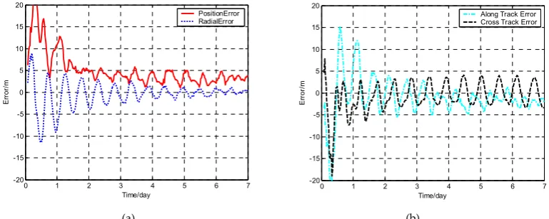
389

(a) (b) Figure 1. Orbit determination errors of SV-01 by WCCEKF algorithm

390

(a) (b) Figure 2. Orbit determination errors of SV-01 by ICEKF algorithm

391

(a) (b) Figure 3. Orbit determination errors of SV-01 by IMCEKF algorithm

0 1 2 3 4 5 6 7 -20

-15 -10 -5 0 5 10 15 20

Time/day

E

rro

r/

m

PositionError RadialError

0 1 2 3 4 5 6 7 -20

-15 -10 -5 0 5 10 15 20

Time/day

E

rro

r/

m

Along Track Error Cross Track Error

0 1 2 3 4 5 6 7 -20

-15 -10 -5 0 5 10 15 20

Time/day

E

rro

r/

m

PositionError RadialError

0 1 2 3 4 5 6 7 -20

-15 -10 -5 0 5 10 15 20

Time/day

E

rro

r/

m

Along Track Error Cross Track Error

0 1 2 3 4 5 6 7 -20

-15 -10 -5 0 5 10 15 20

Time/day

E

rro

r/

m

PositionError RadialError

0 1 2 3 4 5 6 7 -20

-15 -10 -5 0 5 10 15 20

Time/day

E

rro

r/

m

(a) (b)

Figure 4. Orbit determination errors of SV-01 by BEKF algorithm

For each method, the orbit determination errors tend to oscillate steadily after poor initial results.

392

However, differences can be observed among four algorithms. To have quantitative comparisons,

393

the root mean square (RMS) of different errors from each method is calculated in stable section. The

394

average RMS for position error, radial error, along-track error, and cross track error from the four

395

methods are shown in Figure 5. It is worth to point out that the average RMS of position error for

396

WCCEKF, ICEKF, IMCEKF, and BEKF algorithms is around 1.6 meters, 4.5 meters, 2.9 meters, and

397

1.9 meters, respectively.

398

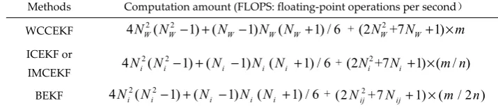
Next, the computation amounts for different methods are summarized in Table 1 and visualized

399

in Figure 6.

400

401

Figure 5. Average RMS of orbit errors

402

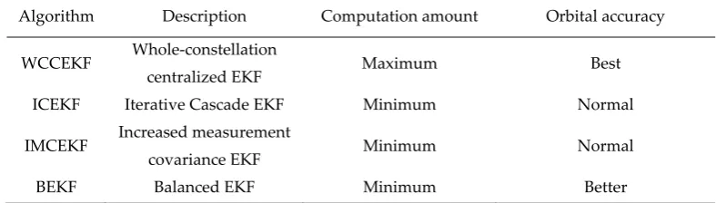
Table 1. Computation amounts, unit: FLOPS ( floating-point operations per second）

403

Methods Computation amount (FLOPS: floating-point operations per second）

WCCEKF 4NW2(NW2 − +1) (NW −1)NW(NW +1) / 6 +

2

(2N_W+7N_W+ ×1) m

ICEKF or IMCEKF

2 2

4N N_i ( _i − +1) (N_i −1)N N_i( _i +1) / 6 + ₍₂ 2_{+7 1) ( / )}

i i

N N + × m n

BEKF 4N Ni2( i2− +1) (Ni −1)N Ni( i +1) / 6 +

2

(2N_ij+7N_{ij+ ×}1) ( / 2 )m n

404

0 1 2 3 4 5 6 7 -20

-15 -10 -5 0 5 10 15 20

Time/day

E

rro

r/

m

PositionError RadialError

0 1 2 3 4 5 6 7 -20

-15 -10 -5 0 5 10 15 20

Time/day

Er

ro

r/

m

Along Track Error Cross Track Error

0 0.5 1 1.5 2 2.5 3 3.5 4 4.5 5

Position Radial Along Trcak Cross Track

RM

S

/

m