226
Copyright © 2018. IJEMR. All Rights Reserved.
Volume-8, Issue-2, April 2018
International Journal of Engineering and Management Research
Page Number: 226-231
ATM Transaction Status Analysis and Anomaly Detection
Yingzhen Lang1 and Wenyuan Sun2
1Student, Department of Mathematics, Yanbian University, CHINA 2
Assistant Professor, Department of Mathematics, Yanbian University, CHINA
2Corresponding Author: [email protected]
ABSTRACT
This article mainly studies ATM transaction feature analysis and anomaly detection. Select the trading success rate, transaction response time and other characteristic parameters, analyze the relationship between transaction response time and transaction success rate. After comparing the fuzzy C-means clustering algorithm and the K-means clustering algorithm, K-means clustering algorithm was used to classify the transaction response time. Thendesign trading anomaly detection program. The use of naive Bayesian classifier for data classification can determine the alarm level. And using Gaussian distribution and Laplace smoothing calibration to increase model accuracy to reduce false alarm. The use of MATLAB programming to get the following result: When the transaction response time is between 0 ~ 85.57, the system predicts to be successful. When the transaction response time between 85.57 ~ 212.31, the system predicts a warning. When the transaction response time between 212.31 ~ 1007.8, the system predicts that the alarm.
Keywords—K-means clustering, Naive Bayes classifier, Laplace smooth calibration
I.
INTRODUCTION
Commercial bank ATM application system includes front and back two parts. Front-end is deployed in the banking department and their service points ATM application system, the back end of the head office data center processing system. The cardholder submits a query, transfer or cash withdrawal service request from the front-end device to the background for processing and returns the processing result to the front end to notify the cardholder of the final status of the business process. Commercial Bank of China headquarters data center monitoring system summarizes some of the transaction statistics, including traffic, transaction success rate, transaction response time. In this paper, we will build a model to construct a certain index to select, extract and
analyze the characteristic parameters of the ATM transaction status. According to the construction index, we design a set of transaction status anomaly detection scheme. Under the condition of the availability of the transaction system, it can promptly report to the police while minimizing false alarms and false warning. So it can improve the success rate of ATMin order to benefit the people.
II.
SELECT, EXTRACT, AND
ANALYZE THE CHARACTERISTIC
PARAMETERS OF ATM TRANSACTION
STATUS
Business volume refers to the total number of transactions that occur every minute, including the success of the transaction and the status of abnormal transactions. Because the data have little effect on the problem, do not analyze it.
Transaction success rate refers to the number of transactions per minute and the volume of business success. Suppose you can use the success rate of transactions in the problem to estimate the average personal success rateand it is independent. The success rate of the transaction can be reasoned out whether the response time is abnormal.Therefore it is the main characteristic parameter of the analysis.
227
Copyright © 2018. IJEMR. All Rights Reserved.
Therefore, the main analysis of the relationshipbetween transaction response time and transaction success rate. The transaction response time is divided into grades, to determine the success rate of the current response time level.
III.
CLASSIFICATION
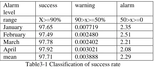
First, according to the success rate, data is divided into three levels: success, warning, alarm [1]. Let x be the success rate of 1 to 4 months given by the success rate of the calculation of the data. The results are as follows Table 3-1
Alarm level
success warning alarm
range X>=90% 90>x>=50% 50>x>=0
January 97.65 0.007719 2.35
February 97.49 0.002480 2.51
March 97.78 0.002402 2.21
April 97.92 0.003021 2.08
mean 97.71 0.003888 2.29
Table3-1 Classification of success rate
Through the program from January to April, the success rate is calculated. And take the average, get the prior probability of success, warning, alarm. Use the mean
formula
n
x
x
x
x
1
2
n_
(3.1)
The success rate at success and warning levels is calculated by subtracting the ratio between success and warnings from 1 to arrive at the alarm rate. Due to the huge amount of data, we have prepared two clustering methods to divide the time. The response time characteristics are divided into five categories, representing different intervals respectively, which are fuzzy C-means clustering algorithm and K-means clustering algorithm .
3.1 Using fuzzy C-means clustering algorithm to classify the time level
Clustering analyzes the patterns of data and groups the data into categories based on the similarity of the patterns. Categories can be precise in nature, or they can be vague. Clear and fixed boundaries are defined between exact categories, while ambiguous boundaries are not clear.
In fuzzy clustering, a point in a dataset may belong to different categories with different degrees of membership. The metric of pattern similarity can be calculated by using the included cosine of the distance feature vector. Consider N L-dimensional data points, denoted as i = 1, 2, ..., N. Each data point is characterized by an L-dimensional vector, ie
)
,
,
,
(
i1 i2 ili
x
x
x
x
(3.2)
The response time characteristics are divided into five categories that C = 5. (In principle, 2 <= C <= N). The membership matrix is characterized by [μ], the dimensions
of which are N * C, where the elements
u
ij
0
,
1
and1
1
c
j ij
u
, minimize the global cost function
21 1
,
F
ijc
j N
i g ij
d
u
c
u
(3.3)
Among them,
d
ij
c
j
x
i (3.4)g is a free function used to control the degree of mixing of different categories. When g = 0, each sample of the criterion belongs to only one cluster. When g> 0, the criterion allows each sample to belong to multiple clusters. Minimize the global cost function to satisfy the constraint,
for any
i
,1
1
c
j ij
u
(3.5) The cost function is rewritten as
cj N
i
N
i
c
j ij i ij
g ij
N
u
d
u
c
u
F
1 1 1 1
2 ,
1
,
)
1
.
0
,
,
(
(3.6) The argument will be differentiated to zero
Solve it:
2 1 1
1
1
1
,
(
)
ij cij g
m im N
g ij i i
j N
g ij i
i j
d
d
x
cc
j
(3.7)
According to the above algorithm, we use Matlab to process the transaction data from January to April. Because the C-means clustering is fuzzy clustering, the answers are different each time. Table 3-2 shows the time division of January in 3 times.
The first sort
Theseco nd sort
The third sort
The fourth sort
The fifth sort first
time
68.79 96.45 88.45 101.62 75.57
second time
97.56 103.54 72.25 88.16 94.26
third time
88.15 89.85 97.15 106.78 82.64
228
Copyright © 2018. IJEMR. All Rights Reserved.
From the results of the above table, it can be seenthat the results of fuzzy C-means clustering are changed every time, and there is no regularity at all. Therefore, the clustering can not be performed well. Each group of data has a big difference and has no reference value.
3.2 Use K-means algorithm to classify transaction response time
K-means clustering is the most well-known clustering algorithm [2], and it is the most widely used in all clustering algorithms for its simplicity and efficiency. Given a set of data points and the number of clusters k needed, k is specified by the user and the k-means algorithm repeatedly divides the data into k clusters according to a distance function. Then calculate the distance between each seed cluster center and each object, and assign each object to the nearest seed cluster center. Clustering centers and the objects assigned to them represent a cluster. When all objects are assigned, each cluster center is recalculated based on the existing objects in the cluster. This process will be repeated until a certain termination condition is met. The termination condition can be that no object is reassigned to a different cluster, no clustering center will change again, and the sum of square errors and local minimum.
Given the observation set
(
x
1,
x
2,
,
x
n)
, eachobservation is a d-dimensional real vector, and K-means clustering divides these n observations into k sets
respectively,
k
n
, so as to minimize the sum of squares in the set. In other words, its goal is to meet the following equation:2
1
min
arg
k
i x S i s
i
u
x
(3.8)
Where
u
i is the mean of all points inS
iInitialization: Randomly select K cluster mean
j
m
,
j
1
,
k
; we intend to divide the time into five categories, K = 5;Loop until K mean no longer change so far:
k
j
C
j
,
1
,
,
(3.9) for
i
1
ton
i k k j ijk
x
m
C
C
x
k
arg
min
,
1
(3.10) end for
Update the mean of K clusters:
K
j
n
x
m
j C x jj
,
,
1
,
(3.11) Output: Clustering
C1,Ck
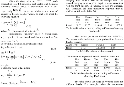
Since MATLAB has a function for solving means, we can calculate the result directly. Because the K-means clustering algorithm belongs to the precise clustering, results are same. The transaction response time in the transaction data from January to April in the title is divided. The results of the division are shown in Table3-3.
The first sort
Thesec ond sort
The third sort
The fourth sort
The fifth sort January 69.05 89.44 105.53 212.31 1007.8 February 80.55 102.72 1240.7 3082.8 6856.7 March 85.27 114.22 2399.5 2285.8 4967.9 April 87.01 121.44 3236.2 11229 50315
Table 3-3 classifies time by K-means clustering
In the data in the above table, from the beginning of February, there is a mutation in the third level. The data given in the observation shows that the response time is less than 1000ms. If the transaction response exceeds 60s,time must be abnormal which is impossible to happen, so the first type of choice for the first class in January. Because the smaller can reflect the data, the first category from February to April is more in line with the second category from January. And we can average them. The second category from April to April is more consistent with the third category in January, so they are averaged, too. Therefore, the final transaction response time is divided as follows in Table 3-4.
The first sort
Thesec ond sort
The third sort
The fourth sort
The fifth sort Result 69.05 85.57 110.98 212.31 1007.8 Table 3-4 Divide the time according to K-means clustering
Final results
The success grades are divided into Table 3-5, The results in the table are the prior probabilities for each level of success.
Alarm level success warning alarm Result 97.71 0.003888 2.29
Table 3-5 Classification of success rat
The transaction response time is divided into Table 3-6 The
first sort
Thesec ond sort
The third sort
The fourth sort
The fifth sort Result
0-69.05
69.05-85.57
85.57-110.98
110.98-212.31
212.31-1007.8 Table 3-6 classifies the time according to K-means
clustering Final result
229
Copyright © 2018. IJEMR. All Rights Reserved.
response time of a piece of data is 88.05 ms, itslevel oftransaction response time is the third type.
IV.
DESIGN TRANSACTION STATUS
ANOMALY DETECTION PROGRAM
Design a set of transaction status anomaly detection scheme, which can achieve timely alarm when the application availability of the transaction system is abnormal, and minimize the false alarms and false warning. Assuming that the success rate is independent of transaction response time, based on the above conclusion, we use Naive Bayesian classifiers to classify the data to determine the response time to determine the alert level.
Bayesian decision theory [2] is a basic method in statistical pattern recognition. Bayesian decision-making theory is necessary for the preparation of naive Bayesian classification. The main work is to determine the characteristics of the attributes according to the specific circumstances. Each feature attribute is appropriately divided.Then part of the classification of items to be classified by classification to form a training sample set. All the data to be classified in this phase is input, and the attribute and training sample are output. The frequency of occurrence of each category in the training sample is then calculated. Conditional probability is estimated for each category, and the result recorded. Finally,the task is to use the classifier to classify the classification of the input, which is the classifier and to be classified. The output is to be classified and the type of mapping.
Assuming pattern of the characteristic vector is x, the purpose of the classifier is to classify it as one of the
categories
w
1,
w
c.1. Class Prior Probability
P
(
w
i)
The prior probability is the probability that a category
i
w
will occur because the classifier can only determine the sample x as one of the c categories, so
1
)
(
1
c
i i
w
P
(4.1) If there is no information about the knowledge model itself and the feature vector x is not generated, it is still necessary to classify it. Discrimination is based on the prior probability of each category.
2. Posterior probability
P
(
w
i|
x
)
The pattern recognition system always obtains some information of the pattern to be recognized and generates the feature vector x. In this case, the probability of occurrence of each category can be analyzed under the condition of the known feature vector x. Therefore, the pattern recognition system is based on not only the priori probability but the posterior probability.
3. The conditional probability density
P
(
x
|
w
i)
Classifiers need to be classified according to the size of the posterior probability. However, in reality, the posterior probability is often not directly available. The prior probability of each class and the conditional
probability density function
P
(
x
|
w
i)
of each class canbe obtained.
The relationship between posterior probability, prior probability and conditional probability is Bayesian formula
)
(
)
(
)
|
(
)
|
(
x
p
w
p
w
x
p
x
w
p
i ii
(4.2)
In the type,
p
(
x
)
is a priori probability density of sample x.Bayesian classifier is classified according to the posterior probability of the input mode x, which is identified as the category with the highest posterior probability. In practical calculation, the posterior probability is transformed into a priori according to the Bayesian formula Probability and the conditional probability density product.
Secondly, we use Gaussian distribution as a Bayesian classification probability model.
Gaussian density function ofthe single factor:
2 22
exp
2
1
)
(
u
x
p
x
p
(4.3) Where mean
and variance2
are parameters of Gaussian distribution. If there are n samples)
,
,
,
(
x
1x
2
x
n, obeying this Gaussian distribution, you can make an estimate of the mean and variance:
ni i
x
n
u
1
1
ni
i
u
x
n
12 2
)
(
1
(4.4) The expression of multivariate Gaussian density function is
11
2 2
(x
)
1
(x)
exp
2
(2 p) |
|
T
d
x
p
(4.5)
The vector
x
R
d, and distribution parameters are the mean vector μ and the covariance matrix Σ, whichcan be estimated by samples
(
x
1,
x
2,
,
x
n)
which230
Copyright © 2018. IJEMR. All Rights Reserved.
n i ix
n
u
11
, T i n ii
u
x
u
x
n
(
)
(
)
1
1
(4.6)Assuming the classification of
c
categories, the priori probabilities of the categories are that the samples of each category following the Gaussian distribution. The logarithmic function is a monotonically increasing function, so taking the logarithm of the Distinguish function does not change the magnitude of the Distinguish function value for each category. The density function of the Gaussian distribution is an exponential function. For convenience of calculation, the Distinguish function in the formula can be transformed into a logarithmic Distinguish function:
(x)
ln
(x |
) P( )
ln (x |
) ln ( )
i i i i i
g
p
P
P
(4.7) Substituting the Gaussian density function yields:
1
1 1
(x) (x ) ( ) ln(2 p) ln | | ln ( )
2 2 2
T
i i i i i i
d
g
x
P(4.8) Then, use the general Gaussian distribution, ignoring the category-independent terms, expand (4.9) to (4.10).
1 ) ( ln ln 2 1 2 ln 2 ) ( ) ( 2 1 ) (i i i i
T i
i p P w
d u x u x x g (4.9) ) ( ln ln 2 1 2 1 2 1 )
( 1 1 i
i i T i i T i i T
i x x x u x u u P w
g
(4.10) Make
1
1
2
iW
,
1
i i i
w
0
1
1
ln |
| ln (
)
2
2
T
i i i
P
i
There is a standard form of the second Distinguish function:
0
)
(
x
x
TW
ix
w
Tix
w
ig
(4.11) In the above, we assume that the transaction response times are independent and the data are continuous randomly. Therefore, we consider the transaction response time satisfies the Gaussian distribution. We can classify the data using naive Bayesian classifier.In the ATM transaction state feature analysis, because the number of recognition features in the problem is relatively small and the number of training samples is relatively large, an effective way to solve the Bayesian classification with multi-feature and less-sample is to use the naive Bayesian classifier. We use naive Bayesian classifier. A basic assumption of Naive Bayesis that all
features are independent of each other under the condition that the category is known,
d j i j i di
p
x
x
w
p
x
w
w
x
p
1
1
,
|
)
(
|
)
(
)
|
(
(4.12) When constructing a classifier, the conditional probability density of each class can be obtained by simply estimating the distribution of each class's training samples on each dimension feature one by one, which greatly reduces the number of parameters to be estimated.
Naive Bayesian classifiers can determine the distribution of samples in each dimension based on the specific problem. Suppose each class sample obeys the independent Gaussian distribution of each dimension, which is the most commonly used one hypothesis, we can get the function (4.13).
2 21 1
1
(x | ) (x | ) exp
2 2
d d
j ij
i j i
j j ij ij
x p p p
(4.13) In the formula, the mean value of the I dimensionin the j dimension is
u
ij , 2ij
represents the corresponding variance. This can be logarithm distinguish function:
2 2 1 2 2 1 1ln
|
lnP
1
ln 2
ln
ln
2
2
ln 2
ln
ln (
)
2
2
i i i
d j ij ij i j ij d d j ij ij i
j j ij
g x
p x
x
P
x
d
P
(4.14) The first of which has nothing to do with the category, can be ignored, resulting in a distinguish function:
d j ij ij j d j ij iu
x
w
P
x
g
1 2 2 12
)
(
ln
)
(
ln
)
(
(4.15)Because the characteristics of the data only one-dimensional transaction response time, it is a Gaussian distribution of the single factor. Assuming a total of N samples, of which M samples success,
n
1samples response time for the i-level, andn
2samples ofn
1 response time for i-level success.231
Copyright © 2018. IJEMR. All Rights Reserved.
B = {choose a sample from any trading success rate for thej-level}
N
n
A
P
1)
(
N
M
B
P
(
)
)
(
)
(
B
|
A
P
)
(
)
|
(
)
|
(
A
P
B
P
A
P
B
A
P
A
B
P
(
)
(4.16)
Since
P
(
A
)
is a constant, we do not consider, we get the following formula:)
(
)
|
(
)
|
(
B
A
P
A
B
P
B
P
(4.17)
Since A and B events are independent, the naive Bayesian classifier[3] is the following formula.
)
(
)
(
)
|
(
B
A
P
A
P
B
P
(4.18)However, there is 0 when calculating a priori probability, so we use Laplace smoothing. Laplace smoothing refers to the fact that when a feature does not appear under a category, it is still possible to get a high probability that X belongs to category
Ci
, even though there is no such probability. To avoid this problem, one can assume that the training database D is so large that variations in the estimated probabilities resulting from adding 1 to each count are negligible. However, it is convenient to avoid the probability value of 0. This probability estimation count is called Laplace calibration.1
1
N
n
L
(4.19) n is the number of samples under category i, and N is the total number of samples.
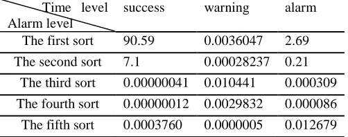
According to the above algorithm, we use MATLAB programming of alert level and response time level[4] in order to get the following results. (The results of four months is written into an Excel table, the final result)
Time level Alarm level
success warning alarm
The first sort 90.59 0.0036047 2.69 The second sort 7.1 0.00028237 0.21
The third sort 0.00000041 0.010441 0.000309 The fourth sort 0.00000012 0.0029832 0.000086 The fifth sort 0.0003760 0.0000005 0.012679
Table 4-7 Naive Bayesian Classifier Results
According to the above results, we can establish the following alarm model.
The first sort
Thesec ond sort
The third sort
The fourth sort
The fifth sort Range
0-69.05
69.05-85.57
85.57-110.98
110.98-212.31
212.31-1007.8 Result success success warning warning alarm
Table 4-8 Alarm Model
According to the above results, when the transaction response time is between 0 ~ 69.05ms, the system will predict the success. When the transaction response time between 69.05 ~ 85.57 ms, the system predicted a success. When the transaction response time between 85.57 ~ 110.98 ms, the system predicts a warning. When the transaction response time between 110.98 ~ 212.31 ms, the system predicts a warning. When the transaction response time between 212.31 ~ 1007.8ms, the system predicts that the alarm [5].
V.
CONCLUSION
ATM is a technology of information transfer mode, which uses a small packet to carry user data. All kinds of operations are designed around the exchange and processing of cells. Because of the independent operation of ATM, it can enter crowded places such as residential areas, schools and shopping malls to facilitate people's life and work. The ATM transaction anomaly detection program is to perfect ATM system. In the abnormal trading system, it can alarm in time and reduce false warning,improve the efficiency of public transactions.
REFERENCES
[1]Liu Jiafeng, Zhao Wei & Zhu Hailong. (2014). Pattern recognition[M]. Harbin: Harbin Institute of Technology Press.
[2]Zhao Yuan,Wang Jie,&Xiong Yanjiao,et al. (2016). A gaussian mixture model of multivariables in power system reliability assessment. Automation of Electric Power Systems, 40(1), 66-71,80.
[3]Saunders C.S.(2014). Point estimate method addressing correlated wind power for probabilistic optimal power flow. IEEE Transactions on Power Systems,29(3), 1045-1054.