The SOS Platform: Designing, Tuning and Statistically Benchmarking Optimisation Algorithms

(1)

The SOS Platform: Designing, Tuning and

Statistically Benchmarking Optimisation Algorithms

Fabio Caraffini

Institute of Artificial Intelligence, School of Computer Science and Informatics, De Montfort University, Leicester (UK); [email protected]

Abstract:The Stochastic Optimisation Software (SOS) is a Java platform facilitating the algorithmic design process and the evaluation of metaheuristic optimisation algorithms. It reduces the burden of coding miscellaneous methods for dealing with several bothersome and time-demanding tasks such as parameter tuning, implementation of comparison algorithms and testbed problems, collecting and processing data to display results, measuring algorithmic overhead, etc. SOS provides numerous off-the-shelf methods including 1) customised implementations of statistical tests, such as the Wilcoxon Rank-Sum test and the Holm-Bonferroni procedure, for comparing performances of optimisation algorithms and automatically generate result tables in PDF and LA_{TEX formats; 2)}

the implementation of an original advanced statistical routine for accurately comparing couples of stochastic optimisation algorithms; 3) the implementation of a novel testbed suite for continuous optimisation, derived from the IEEE CEC 2014 benchmark, allowing for controlled activation of the rotation operator. each testbed function. Moreover, this article comments on the current state of the literature in stochastic optimisation and highlights similarities shared by modern metaheuristics inspired by nature. It is argued that the vast majority of these algorithms are simply a reformulation of the same methods and that metaheuristics for optimisation should be simply treated as stochastic processes with less emphasis on the inspiring metaphor behind them.

Keywords: algorithmic design; metaheuristic optimisation; evolutionary computation; swarm intelligence; memetic computing; parameter tuning; fitness trend; Wilcoxon Rank-Sum; Holm-Bonferroni; benchmark suite

1. Introduction

Experimentalism plays a major role in all fields of metaheuristic optimisation, as e.g. evolutionary computation (EC) and swarm intelligence (SI), and can be a time-demanding, repetitive and tedious process when required to fine-tune optimisers, compare them or to validate new algorithmic strategies on benchmark problems. Due to their stochastic nature, and the lack of theoretical knowledge on the internal dynamics of many of these nature-inspired approaches, their algorithmic design is partially blind and often empirically performed through a series of trial-and-error phases [1]. This involves using several artificially build benchmark problems, simulating characteristics present in real-world scenarios, but for which some knowledge is available. The use of such testbed problems is preferable since they usually have a more reasonable execution time than real-world applications, they can be run any machine, this being e.g. a modest personal computer or a high-performance computing system, and they are not subject to time and other limitations typical of real-world scenarios if not purposely imposed to reproduce a specific situation. Thus, these problems are suitable choices for performing the algorithmic design phase of novel algorithms and evaluating the performances of specific operators and algorithmic variants. By design, these problems display particular characteristics reported in the corresponding technical reports in term of (e.g. ill-conditioning, separability, m-separability, noisy functional landscapes, modality (i.e. multimodal or unimodal function) etc., allowing also for studying the algorithmic behaviour of certain operators [2–4]).

(2)

In this light, the research community benefits from platforms featuring a large number of algorithms and benchmark testbed problems, as e.g. the Decision Tree for Optimization software [5], COCO [6], IOHprofiler [7] and jMetal [8], which facilitate this testing. However, the availability of code implementing complete of benchmark suites and popular optimisation algorithms is only one amongst the many “tools” required by an algorithm designer to work efficiently and productively focus 100% on algorithmic issues rather than having to deal with the implementation of ancillary software. Useful off-the-shelf methods that a research-oriented platform for metaheuristic optimisation should at least have are:

• performance evaluation methods, based on metrics as algorithmic overhead, scalability, best results, average best result, convergence (e.g. in terms of fitness and population diversity [9,10]), structural bias [1,11] etc.;

• statistical methods for comparing the performances of algorithms [12,13]; • results visualisation methods (in both table and graphical formats);

on top of providing

• a vast and heterogeneous number of benchmark functions and real-world testbed problems; • several state-of-the-art algorithms to be used for comparisons with newly designed optimisation

strategies;

• libraries with implementations of the most popular algorithmic operators such as mutation methods, crossover methods, parent and survivor selection mechanisms, heuristics seleection methods for memetic computing (MC) and hyperheuristic approaches, etc;

• utility methods for generating random numbers, solutions or population of solutions, keeping track of the best newly found solutions and save them to plot fitness trends, handling infeasible solutions [1,14,15];

• a system to spread the runs over multiple cores and threads, thus speeding up the data generation process, and automatically collect and process raw data into meaningful information;

and should be based on

• open source software so that researchers can freely use it and build up upon it;

• a simple and flexible structure so that new problems and algorithms can be easily added.

The Stochastic Optimisation Software, henceforth SOS, exhibits the aforementioned key features thus facilitating the design, the evaluation and the use of metaheuristic optimisation algorithms.

(3)

also represents an excellent pedagogical tool for teaching purposes1and can be used to give guidance to students while implementing optimisation algorithms. Researchers willing to collaborate and add code (algorithms, real-world problems, etc.) to the platform are welcome and invited to get in touch to be added to the SOS GitHub repository2. Finally, it is worth mentioning that due to the simplicity in adding problems and algorithms, SOS represents a useful tool for practitioners who might have less interest in the algorithmic design but a high need for off-the-shelf implementations of optimisation algorithms.

2. The SOS platform

For portability reasons, SOS is coded in Java, thus being platform-independent. To speed up the execution of extensive experiments, some benchmark suites are also available in the form of C/C++ written native libraries (compiled for MS Windows, but mainly MAC OS and Linux machines) using the Java Native Interface (JNI). By default, SOS spreads the “runs” (i.e. the optimisation processes in which one algorithm optimises one problem) over the available threads and execute them in parallel. This can results in quite CPU consuming processes that can be avoided, e.g. if the experiment is executed with a laptop or personal computer, by switching to the single-thread mode by means of the setter methodsetMT(boolean MT)of the classExperiment (i.e. its boolean flag variable must be set to false). By looking at [16], one can notice that in its current release, a strong emphasis is given to real-valued box-constrained single-objective optimisation, aka “single-objective continuous optimisation” in the EC community. Nevertheless, SOS can be used for addressing other optimisation domains such as e.g. discrete or combinatorial ones.

2.1. Functional overview

SOS is research-oriented and is designed to have an intuitive structure making it straightforward to use by both expert algorithms’ designers in the research community and, most importantly, by practitioners and doctoral students from different subject fields.

Indeed, to execute an experiment it is sufficient to add a class, which extends the abstract Experimentclass, in the homonym folder (package). Such class will automatically inherit theadd methods, that can be used to add algorithms and problems to the experiment, and other methods to set e.g. the allowed computational budget (by default this is assumed to be equal to 5000×nwithn

being the dimensionality of the problem) and the number of runs to be performed. Subsequently, a mainmethod must be written to launch one or multiple experiments. To do this, the methods of the utility classRunAndStorecan be imported to e.g.

• execute a list of experiments having different budgets, number of runs, problems and algorithms, or the same experiments but repeated for different dimensional values (if the problems are scalable);

• generate log files describing the performed experiments, (this contains the list of problems, problems and corresponding details such as dimensionality, parameter setting, number of runs, etc.);

• store raw data and process them into results tables and plottable formats as shown in section5.

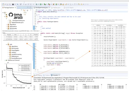
Figure1shows an example of a main method used for executing a list of experiments and display the final outputs, i.e. tables and graphs, generated by SOS after generating and processing the results. Many examples of experiment and main files are present in SOS and can be used as a template to follow for writing new ones. With reference the latest release in [16], a large number of experiment files can be found in theexperimentspackage while several examples of main files (showing different

1 _{Since 2015 its first releases have been used to teach the master module “Computational Intelligence Optimisation” led by} the author of this article at De Montfort University (Leicester, UK).

(4)

configurations and options for storing and processing results in different formats) are available in the mainspackage. However, the most convenient execution point is the classRunExperiments, shown in figure1, which is located in the default package of the SOS platform. More indications on how to write an experiment class are given in section2.2and graphically shown in figure2.

Figure 1.A graphical functional overview of the SOS platform.

To minimise the need for referring to a detailed document, SOS is equipped with a high number of self-explanatory example classes. Moreover, the clear nomenclature used for methods, variable types, class names, and the user-friendly structure of the proposed platform, give guidance to the users, who may not even need further indications. Nonetheless, technical software documentation is made available online to provide users with further information on its packages, classes and methods. Table1displays relevant links to SOS webpages, from where SOS documentation can be accessed. These webpages are be kept up-to-date and the documentation itslef is constantly updated to reflect major changes and evolutions of this software platform. This documentation plays a key role for those who intend to modify SOS source code, extend it or customise it to a specific need.

Description Content Link

SOS webpage software documentation https://sites.google.com/site/facaraff/research/sos

GitHub repository source code https://github.com/facaraff/SOS

Zenodo repository [16] SOS releases https://doi.org/10.5281/ZENODO.3237023

Table 1.Relevant links to source code and software documentation.

SOS makes it very easy to add new algorithms and new problems which are fully compatible with the platform so to exploit its full capabilities. For the sake of good organisation, it is suggested to place their implementation in the three provided packages:algorithms,benchmarksandapplications.

(5)

different combination of variation and/or selection operators thus having a higher number of choices. This results in a good balance between established optimisation methods, as e.g. classic differential evolution (DE) [1,24], simulated annealing [25], genetic algorithms, particle swarm optimisation [26], evolutionary strategies algorithms [27–29], and more modern optimisers as e.g the self-adaptive algorithms in [30–37] and the state-of-the-art memetic algorithm (MA), memetic computing (MC) amd hyperheuristic approaches [3,22,23,38,39]. For a complete list, one can download thealgorithms folder from [16] or check the online documentation. More information on SOS algorithms are given in section2.3.

Thebenchmarksfolder is meant to contain the implementation of problems from established benchmark suites for optimisation. SOS implements several testbed problems and complete benchmarks suites to add in experiment files. A complete list of these optimisation problems and relevant documentation is provided in section3. Furthermore, a novel benchmark suite is presented in section3.1.

Theapplicationsfolder is where specific real-world applications should be implemented. Some examples from the literature, e.g. the code for the application described in [22], and from the suite for real-world problems are available in this folder and downloadable from the repositories indicated in table1.

Theapplications folder is where specific real-world applications should be implemented. Some examples from the literature, e.g. the code for the application described in [22] and for some applications from the suite for real-world problems, are available in this folder.

Following the execution of an experiment, the produced raw data can be processed by means of the classes in the packageutils.resultsProcessing. These provide several functionalities including

• the execution of statistical tests for comparing stochastic optimisation algorithms (described in section4);

• the execution of the novel procedure to compare couples of optimisation algorithms presented in section4.3;

• the generation of plottable files suitable for simple Tikz, Python Matplotlib, Gnuplot or Matlab scripts for displaying best/median/worse/average fitness trends as shown in section5and appendixA;

• the generations of files containing further plottable information such as histograms, relative to final bests distribution amongst several runs, and graphs describing infeasibility and structural bias in optimisation algorithms (see [1,15,40,41] for details);

• the generation of LA_{TEX tables (both source code and PDF files are produced) showing results in}

terms average fitness value (or average fitness error) with corresponding standard deviations and further statistical evidence as explained in section4and graphically shown in in section5.

The fileTabGen.java, located in the Mains folder, contains the methods for generating the previously mentioned tables and graphical outputs and can be modified to customise the production of tables with different layouts and informative content as discussed in section5.

It is worth stressing the fact that having a fast way to visualise results in multiple formats is key to performing many research activities. As an example, when writing papers, it is very useful since raw data are automatically processed and the LA_{TEX source for the comparative tables, to be copied and}

pasted in the main draft, is generated in a few seconds.

(6)

the design phase. To some extents, this problem can be considered dual to the training process in machine learning.

In this light, the algorithmic design process is not very different to the process performed to choose the less disruptive correction method for handling infeasible solutions generated while addressing a problem [1,15,40] and to the fine-tuning process performed to find the most appropriate set of parameters for an algorithm A meant to address specific problem P.

2.2. Parameters fine-tuning

Metaheuristics for optimisation must be tuned on the problem at hand to make them achieve their full potential and return high-quality solutions. Against the original common belief that a “universal” algorithm could have been designed, theoretical achievements such as, first and foremost, the “no free lunch theorems” (NFLTs) for optimisation [42,43] highlighted the need for fine-tuning, self-adaptation and the use of problem-specific operators.

However, finding the optimal parameter configuration is an optimisation problem itself. Despite meta-optimisation strategies have been proposed [44,45], these do not completely solve the problem and are arguable since introducing further complexity while still needing to tune the meta-optimiser. Furthermore, the fact that most real-world optimisation problems are black-box systems, for which no theoretical information on the fitness function is available, increases the difficulty in finding an exact method for finding the optimal configuration of parameters.

Under these circumstances, the parameters tuning process is necessarily performed empirically, thus resulting in a rather time-consuming and tiresome activity. SOS can be used to significantly accelerate and facilitate this task as 1) the same algorithm can be included multiple times in the same experiment file with different parameters configurations; 2) runs can be spread over the available processors and threads to speed up the generation of results; 3) raw data are immediately statistically analysed and results automatically displayed in compact and still highly informative tables and graphs (examples are provided in section5). Hence, the only portion of code that may be needed to tune an algorithm A on a specific real-world problem P with SOS, is actually the one implementing P.

It must be pointed out that also artificially built testbed problems as those already implemented in SOS, see section3, can play a role in the parameter tuning process. Indeed, studying how the algorithmic behaviour of a metaheuristic algorithm changes under different configurations of its parameters can help shed light on how to perform the tuning process. By using testbed problems, whose mathematical properties (e.g. differentiability, separability, modality, ill-conditioning etc.) are known, we can understand what the effect of the parameters is when the fitness landscape displays particular mathematical features. As a result, specific regions of the parameters space could be detected to obtain a robust general-purpose behaviour rather then a very problem-specific one, or to strengthen exploitation capabilities rather than exploration capabilities, or to minimise the rise of algorithmic structural biases, as done in [1,11,40], the generation of a high number of infeasible solutions, as done in [1,15] or premature convergence [46] and stagnation [47], as done in [10].

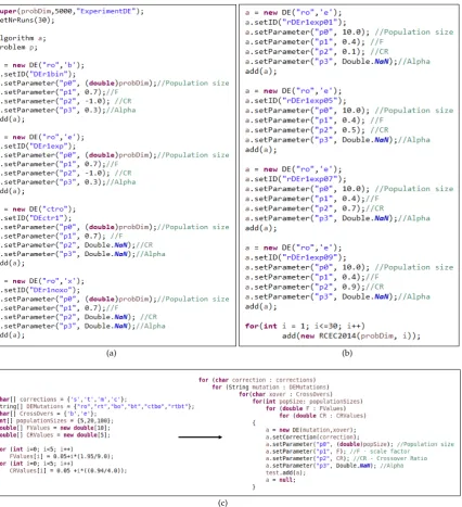
Most of the aforementioned studies have been performed with SOS and their experiment files can be found in [16]. Portions of code from three experiment files are reported in figure2, which helps understand how the parameters space of an algorithm can be explored in SOS.

(7)

(a) (b)

(c)

Figure 2.Examples from experiment classes (original files are downloadable from [16]) for parameter tuning and algorithmic behaviour testing, i.e. the same algorithms are included in the same experiment under different parameters configurations. The fragment of code reported in (a) refers to an experiment performed for the studies in [4,48] located inSOS→src→experiments→rotInvStudy→CEC11.java. The fileRCEC14TuningDEroe.java, from which the segment of code in (b) is taken, can be found in the same folder. In this case, the DE/rand/1/exp algorithm is executes with three different values for the crossover rate parameter Cr over the 30 rotated versions of the problems of the R-CEC14 benchmark suite proposed in this article in section 3.1. Finally, the fragment of code in (c) shows how to compactly define an experiment running 12 DE variants with several different parameters configurations, over one problem only, to find the most appropriate triplet hpopulation size, scale factor (F), crossover ratio (Cr)i. The complete class file for this example is located inSOS→src→mains→ExampleTuning.java.

(8)

read for further details. To execute this experiment with increasing problem dimensionalities, and therefore, in turn, increasing population sizes, it is sufficient to instantiate objects with increasing probDimvalues by calling the class constructor in the fileRunExperiments.java(as shown in the example of figure1). It is interesting to note that, to avoid confusion, a name is assigned to each DE variant ( e.g.a.setID("DErn1bin")). The assigned name will show up in the generated tables. If a name is not provided, as in the example of figure2.2-(c), it will be automatically assigned equal to the class name of the launched algorithm. Therefore, in this case, the assinged names would start with DE, followed by “-i” where “i” represents a counter incremented every time an algorithm is added in an experiment. In a nutshell, if names were not specified in the example of figure2-(a), tables would display DE-1, DE-2, DE-3 and DE-4, since all the algorithms in this experiment are instances of DE class.

Differently, in figure2-(b) the same DE variant, namely DE/rand/1/exp, is added three times in the experiment with three different values for the so-called “crossover ratio” parameterCr. As can be seen at the bottom of the figure, all the 30 rotated problems from the benchmark suite proposed in section3.1are added to this experiment. Hence, its purpose is to understand the impact of theCr

value on DE/rand/1/exp when facing different problems.

Finally, figure2-(c) shows a very compact and fast way for writing a large experiment file in SOS, in which 12 DE variants are equipped with 4 different correction strategies for handling infeasible solutions, for a total of 48 different algorithms to tune. From the left-hand side of the figure it can be seen that the DE variants are obtained by combining the 6 mutations with the 2 crossover operators in theDEMutationsandCrosOversarrays respectively. The 4 correction strategies are in thecorrections array. For details about the adopted notation for DE variants and correction strategies one can consult the articles [1,11] and the results in [41]. For each algorithm, the explored parameters space is defined as the Cartesian product of the three sets represented by thepopulationSizesarray, containing 3 population sizes, theFValuesarray, containing 10 equally spaced values for the so-called “scale factor”

Fin the range[0.05, 2], and theCRValuesarray, containing 5 equally spaced values forCrin the range [0.05, 0.99]. Hence, each one of the 48 algorithms is tuned over a set of 150 possible combinations of the three parameters. In total, this means that 7200×Nroptimisation processes are executed, withNr

being the number of performed runs, for each problem added to this experiment. The full code for this examples, namedExampleTuning, is located in themainspackage. For demonstration purposes,

Nr=10 and the computation budget is kept short, i.e. 1000×n. In a real tuning experiment, this can be increased as required.

2.3. Adding new algorithms and problems

The literature is currently saturated by novel nature-inspired optimisation metaphors claiming to mimic the collaborative or individual behaviour animals [49–56], human activities [57–59] or other natural phenomena [60–62]. The contribution made by most of these new optimisation paradigms is arguable as they are very similar to established frameworks form the field of EA, such as the GA, the DE and the ES ones, and from the field of SI as e.g. the PSO algorithm. Furthermore, all of these new metaheuristics are subject to the NFLTs and cannot outperform classic ones over all possible black-box problems without fine-tuning. It must be remarked that also amongst the most established optimisation frameworks some similarities can be detected in support of the thesis that taxonomies based on metaphor inspiring their design could be indeed avoided. To provide some examples, it is sufficient to observe that DE mutations, being linear combinations of individuals from the population [1,24], operate the same as arithmetic crossovers in real-valued GAs and other EAs [18]. Similarly, it can be observed that the lack of parent selection in SI frameworks, as e.g. the PSO [26], is simply moved in the perturbation operator since requiring the definition of the neighbourhood of the candidate solution to b perturbed to find itslocal bestsolution.

(9)

of the metaphor behind them, all metaheuristic methods are the expression of the same concept and aim at reaching a good balance betweenexplorationof the fitness landscape, looking for promising basins of attraction, and theirexploitation, to refine them and find local optimal points (i.e. maxima or minima according to the need). This dynamic process can alternate such phases as appropriate to keep looking for the global optimum, without prematurely converging to a locally optimal point or stagnating without being able to return any satisfactory near-optimal solution.

Hence, it makes sense to analyse the algorithmic structure of modern nature-inspired optimisation algorithms and extrapolate a common, high level, general skeleton to use as a template for their implementation. This is done in SOS by means of the abstract classAlgorithm, from which all algorithmsinheritancillary and auxiliary methods (e.g. for algorithm execution, storing the fitness trend, setting or generating the initial guess, etc.) andextendonly the parts to be customised to implement the specific optimisation framework (e.g. a GA rather than a DE, a hybrid method or a completely new optimisation paradigm). Therefore, any class file extendingAlgorithmis already equipped with the required methods to be added into an experiment file and be executed as described in the previous section, while it must implement one method, namedexecute, which returns an object of the kindFTrend). To give further details in this regards, other than referring to online software documentation, it is worth briefing about the classes of the packageutilslisted below.

• RunAndStore: this class contains the implementation of all methods involved in executing an algorithm in single or multi-thread modes, collecting the results, display them on a console (unless differently specified) and saving them into text files.

• RunAndStore.FTrend: this class instantiate auxiliary objects storing information collected during the optimisation process and that must be returned by all the algorithms implemented in SOS. As shown in figure3-(b), the primary purpose of these objects is to store the fitness function evaluation counter and the corresponding fitness value in order to be able to retrieve the best (max or min according to the specific optimisation problem) and plot a so-called fitness trend graphs like those in figure1and in figure10of section5. The class provides numerous auxiliary method to return the initial guess, the best fitness value, the median value, and so on. Obviously, the optioned near-optimal solution must be also stored and, if needed, several other extra pieces of information can be added in the form of strings,integerordoublevalues. As an example, in [10], population and fitness diversity measures were collected during the optimisation process. • MatLab: This class provides several methods to quickly initialise and manipulate matrices. These methods include operations between matrices but, most importantly, the auxiliary methods for generating matrices of indices, for making copies of other matrices and decomposing them. • Counter: This is an auxiliary class to handle counters when several of them are required to

e.g. count fitness evaluations, count successful and unsuccessfully steps, etc. In [1,15] this class is used to keep track of the number of generated infeasible solutions how many times the pseudo-random number generator is called in a single run. It must be remarked that for obtaining this information in a facilitated way it is necessary to extend the abstract classalgorithmsISB rather thanalgorithms[16].

Moreover, the packagesutils.algorithmsandutils.randomprovides very useful methods helping users to implement algorithms. These packages contain:

• utility methods for cloning and generating individuals and population in the search space for population-based, single-solution and estimation of distribution algorithms (with a specific package for compact optimisation [63]);

• utility methods for measuring population and fitness diversity according multiple metrics [10] and for manipulating populations into covariance matrices [64,65];

(10)

• therandomutilities, which provides methods for generating random numbers from different distributions, initialising random (integer and real-valued) arrays, permuting the components of an array passed as input, changing the pseudo-random number generator, changing seed, etc.; • a vast number of algorithmic operators (sub-packageoperators) implementing simple local

search routines, restart mechanisms and most importantly

– the classGAOp, which provides numerous mutation, parent selection, survivor selection and crossover operators from the GA literature;

– the classDEOp, which provides all the established DE mutation and crossover strategies plus several others from the recent literature;

– the classes in aos, which implements adaptive heuristic/operator selection mechanisms from the hyperheuristic field [23].

Given the facility in adding new algorithms and the availability of numerous off-the-shelf operators, SOS is a suitable workbench to design hybrid algorithms or variants tailored to the problem at hand. In particular, the possibility of declaring variables of the kindAlgorithm, to initiate and execute optimisation processes inside another algorithm, lead to the implementation of complex algorithms by writing very neat code. This is evident from figure3, where the code of the iterated local search algorithm proposed in [66] is shown. At first glance, one can observe that the source code is clear and resembles pseudocode. Indeed, instead of implementing the sophisticated (1+1)–CMA-ES algorithm in [67], which plays the local searcher role, anAlgorithmvariable is instantiated by using theCMAES_11class available from thealgorithms package and implementing the (1+1)–CMA-ES algorithm. Parameters and computational budget for this algorithm, which can be seen as an operator in this context, are passed as described in the previous sections. It can be noticed that the initial point for each iterated search is passed to the local searcher before it is executed. This point is generated by applying the exponential crossover operator [1] to the current best solution and a feasible randomly sampled individual. Obviously, the crossover method as well as the method for generating an individual in the search space are already present in SOS and therefore are simply imported and used, without the need of writing further code. To monitor the internal dynamic of the resulting algorithm, aFTrendobject can be used as commented in figure3.

(11)

(a) Initialisation phase (b) Optimisation phase

Figure 3.Algorithmic design and implementation in SOS. This example shows portions of code from the algorithm classRI1p1CAMES, located in thealgorithmspackage, which implements the algorithm proposed in [66]. On the left-hand side (a), the initialisation phase, where the algorithmcma11of the kingCMAES_11(which extendsAlgortithms) is initialised and ready to be executed inside another class extendingAlgortithms. On the right-hand side (b), the implementation of an iterated local search method usingcma11as a local. TheFTrendvariableftreturned bycames11is automatically merged to the one of the main algorithm, i.e.FT, to obtain a unique global fitness trend.

3. Benchmarking with SOS

Due to the difficulties in dealing with real-world black-box problems, the metaheuristic optimisation research community started developing artificially built functions [68] to

• significantly reduce the optimisation time;

• investigate algorithmic behaviours over problems with known or partially known characteristics and properties;

• be able to empirically study the scalability of optimisation algorithms.

(12)

To remove the burden of implementing such a high number of testbed problems, the SOS platform comes with full implementations of:

• several basic testbed problems as those in [20];

• several complete benchmark suites amongst those released over the years for competitions on real-parameter optimisation at theIEEE congress on evolutionary computation(CEC), namely

– CEC 2005 [69];

– CEC 2008 (for Large Scale Global Optimisation) [70]; – CEC 2010 (for Large Scale Global Optimisation) [71]; – CEC 2013 [72];

– CEC 2013 LSGO (for Large Scale Global Optimisation) [73]; – CEC 2014 [2];

– CEC 2015 [74];

• the fully scalable test suite for the special issue of soft computing (SSCI) 2010 onscalability of evolutionary algorithms and other metaheuristics for large scale continuous optimization problems[75]; • a stand-alone implementation of theblack-box optimization benchmarking(BBOB) suite [76] as well as all the BBOB suites included in the 2019 release of the COCO platform [6] (which is internally called by SOS);

• a novel variant of the CEC 2014 benchmark, named “R-CEC14”3, presented in section3.1.

It is worth indicating that some applications from the CEC 2011 benchmark suite for real world optimisation [77] are implemented in theapplicationspackage.

3.1. The R-CEC14 benchmark suite

The original IEEE CEC 2014 benchmark suite [2] consists of 30 challenging functions for single objective real-parameter numerical optimisation. These problems are obtained by shifting, rotating and ill-conditioning well established classical functions in the fields of computational optimisation. Only 2 of the 30 mathematical functions are not subject to rotation, i.e. function number 8 (Shifted Rastrigin’s Function) and function number 10 (Shifted Schwefel’s Function), but do have a rotated counterpart in the benchmark suite.

For this reason, one could argue that only these 4 functions, i.e. number 8, 10 and the 2 rotated versions, are insufficient to draw interesting conclusions on

• the efficacy of so-called rotation invariant operators in optimising rotated and unrotated landscapes, as done in [48] and [4] for DE, which unveiled no differences in the performances of such operators over the two classes of problems4;

• separability and degrees of separability, measured e.g. with the separability index proposed in [3], as well as on the suitability of certain algorithms and algorithmic operators for addressing separable and non-separable problems.

Indeed, rotating a separable function does not alter its modality or ill-conditioning features, but does alter its separability. In this light, while working on the study in [48] I redesigned the original CEC 2014 and implemented a Java version in which the rotation operator can be activated and deactivated by simply setting the integer rotation (R) flag. If equal to 1, the rotation operator is active and the functions are identical to those of CEC 2014. Conversely, if null, no rotation takes place. To avoid duplicates, functions 8 and 10 are removed since obtainable from their rotated counterparts, i.e. functions 9 and 11, by setting the rotation flag equal to 0.

3 _{The R indicates a rotation flag used to activate or deactivate the rotation operator.}

(13)

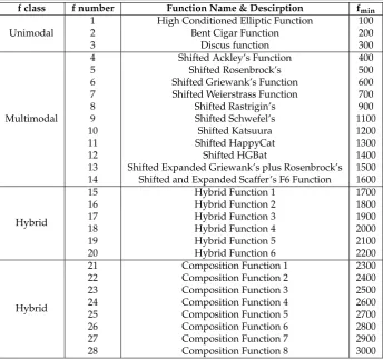
Thus, the resulting R-CEC14 suite contains 56 functions:

• the first 28 are the functions listed in table2, whose analytical expressions can be found in [2]; • the last 28 functions are their rotated versions.

These problems are optimised within an hypercubical search space D defined

as [−100, 100]n, with n ∈ [10, 30, 50, 100] being the admissible dimensionality values.

For each problem, the corresponding n × n rotation matrices are stored in the

benchmarks.problemsImplementation.CEC2014.files_cec2014package [16] and loaded when the rotation operator is active. The minimum fitness function value fmin = min

x∈Df(x) = f(xmin), with

xmin=argmin x∈D

f(x), is shown in table2and more detailed information on the functions can be found in [2] or by controlling the source code [16] and SOS online documentation.

f class f number Function Name & Descirption fmin

Unimodal

1 High Conditioned Elliptic Function 100

2 Bent Cigar Function 200

3 Discus function 300

Multimodal

4 Shifted Ackley’s Function 400

5 Shifted Rosenbrock’s 500

6 Shifted Griewank’s Function 600

7 Shifted Weierstrass Function 700

8 Shifted Rastrigin’s 900

9 Shifted Schwefel’s 1100

10 Shifted Katsuura 1200

11 Shifted HappyCat 1300

12 Shifted HGBat 1400

13 Shifted Expanded Griewank’s plus Rosenbrock’s 1500 14 Shifted and Expanded Scaffer’s F6 Function 1600

Hybrid

15 Hybrid Function 1 1700

Hybrid

21 Composition Function 1 2300

Table 2. R-CEC14 problems list. Each problem can be evaluated with and without the action of the rotation operator. Technical details on these problems and the rotation procedure are available at [2].

(14)

4. Statistical analysis with SOS

Stochastic algorithms can be evaluated e.g. by measuring their overhead5, by calculating their time and memory complexity, in terms of scalability, average performances (i.e. final fitness value returned averaged over multiple runs) and, qualitatively, by visual inspection of fitness trend graphs. However, to be able and claim that an algorithm is capable of outperforming one, ore more algorithms, when tested on a specific problem, or a set of multiple problems, statistical evidence must be sought.

A review of potential statistical tests to be used for analysing and comparing stochastic algorithms was published in [12]. Amongst the suggested methods,non-parametrictests such as the Holm test [78] and the Wilcoxon Signed-Ranks test [79] soon became the most employed since results collected over multiple runs are not necessarily normally distributed. Several recent studies adopted similar variants of these methods, namely the Wilcoxon Rank-Sum test and the Holm-Bonferroni test, which can now be considered quite established in the field [3,4,23,39].

To facilitate the use established and advanced statistical tests for evaluating performances of stochastic optimisation algorithms, SOS provides implementations of

• a comparison test based on the Wilcoxon Rank-Sum test as described in section4.1 • a comparison test based on the Holm-Bonferroni test as described in section4.2; • the Advanced Statistical Analysis (ASA) test proposed in section4.3.

4.1. The Wilcoxon Rank-Sum test for stochastic optimisation

The Wilcoxon Rank-Sum test [80], aka Mann–Whitney U test [81], is a non-parametric test used to understand whether two independent samples belong to populations having the same distribution. Unlike similar parametric counterparts, as e.g. the popular two-sample unpaired t-test [82], it does not operate on data but scores, referred to asranks, associated to the acual values and for which assumptions on their distribution can be made. This makes it suitable for analysing results of stochastic algorithms, whose distributions may significantly vary over different problems and combinations of parameters, while their ranks distributions can be assumed to follow a normal model.

To describe the procedure implemented in SOS, let us consider two generic algorithms A and B run on a generic problem P for nAand nBtimes respectively6. Thenull-Hypothesisis then formulated

as H0: A=B which means that, regardless of their working logic, the two algorithms are statistically

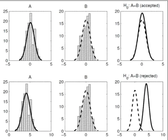
identical, i.e. they are instances of the same population as the solutions provided over multiple runs are equally distributed. This is graphically shown in figure4. The Wilcoxon Rank-Sum test can then be used to produce evidence to reject H0. Failing this task would instead support the so-called alternative

hypothesis, which is formulated as H1: A<B or H1: A>B, if a one-sided (aka one-tailed) test is

performed, or H1: A6=B, if a two-sided (aka two-tailed) test is performed.

By default, SOS performs the two-tailed variant. However, both the one-sided variants and the two-sided variant are implemented and usable. Indications on how to run this test in SOS are in the online documentation and an example is also displayed in figure7. Regardless of the used variant, i.e. single or two sided, the null hypothesis has always the same formulation and can be either accepted or rejected as shown in figure4. Conclusions can then be drawn from the outcome of the test in terms of performances for A and B. For example, if H0: A=B is rejected in a two-sided execution of the test,

indicators such as the average fitness value or the median fitness value over the performed runs can be used to understand which algorithm outperform the other on the problem P. Obviously, this is not needed the two one-sided variants are considered.

The steps in sections4.1.1to4.1.5describe the decision-making process implemented in the SOS platform.

5 _{In SOS the class}_{mains.test.TestOverhead}_{can be used for this purpose.} 6 _{Usually, n}

(15)

Figure 4.Hypothesis testing. On the top row, the the test fails at rejecting the null-hypothesis (i.e. H0 is accepted) as the algorithms A and B have significantly similar distributions. On the bottom row, H0 is rejected as A and B are two different stochastic processes with significantly different distributions.

4.1.1. Reference and comparison algorithms

To be perform a statistical test, a “reference” is needed. When asked to perform the Wilcoxon Rank-Sum test on the results generated with an experiment E, the list of algorithms executed in E is shown and the reference can be indicated. If not specified, SOS assumes that the reference algorithm is the first that was added in E. Without a loss of generality, let us conceptualise A as the reference algorithm. The remaining algorithms in E will form a set of “comparison” algorithms. If more than two comparison algorithms are present, SOS will iteratively schedule a Wilcoxon Rank-Sum test to compare the reference algorithm A with each comparison algorithm B, taken from such set, for each problem P in E. The selection order of each comparison algorithm can be specified. This will be the order of appearance for the algorithms on the automatically generated result table, as those shown in the graphical examples included on section5. By pressing “c” during the selection process, a table will be created even though the comparison set is not empty. This way, multiple and smaller results tables can be generated from a single experiment. If the “a” (i.e. all) option is insted used, a single long table for the whole experiment E will be generated. This will containing as many columns as algorithms in E and as many rows as problems in E.

4.1.2. Assigning ranks

Let us consider the totality of the observations obtained from the N=nA+nBruns. Without a

loss of generality, let us refer to a minimisation problem, for which the lower the fitness value the better the algorithm’s performance. Observations are then sorted with ascending order to assign ranksri=i

(withi=1, 2, 3, . . . , N) so that the smallest value has rank 1 (i.e.r1=1), the second smallest value has

rank 2 (i.e.r2=2), and so on to get to the observation with the greatest value, having a rankrN =N).

(16)

good representation of the real distribution, these four ties will be assigned with the same rank value

rj = 4+5+46+7 =5.5 (j∈ {4, 5, 6, 7}).

4.1.3. The rank distributions

Let us indicate with WAthe random variable associated with A. Its distribution of probability

is tabulated only for small sample sizes [83], i.e. N < 20, which is very small and unusual for an optimisation experiments. Hence, SOS must implement such distribution to deal with larger sample sizes and get more accurate evaluations results. To do this, see [80,83], it is sufficient to define the normal distributionN(µA,σA)whose mean valueµAand standard deviationσAare calculated with

µA= r

nAnB

N+1

12 and σA=nA

N+1 2

respectively.

4.1.4. Wilcoxon rank-sum statistic and p-value

Let us fill a setRAwith the nAranksriassociated to the observations from the reference algorithm.

The so-called Wilcoxon rank-sum statisticwAis calculated by summing all the values as indicated

below

wA=

∑

r∈RA

r

and use it to define the p-value. For the default case, i.e. two-sided analysis with H0: A =B

versus H1: A6=B, this is formulated as follows

p-value=   

 

2·Prob{WA≥wA} ifwA>µA (i.e.wAis in the upper tail)

2·Prob{WA≤wA} otherwise (i.e.wAis in the lower tail)

where the probability of falling into the tail of the distribution closest towAis doubled in order to consider both the cases in which the two algorithms differ because A>B and A<B simultaneously. This is not needed for the one-sided, for which the null hypothesis H0: A=B is either tested against

the alternative hypothesis H1 : A < B, with a corresponding p-value= Prob{WA ≤ wA}, against

the alternative hypothesis H1: A>B, with a correspond p-value=Prob{WA ≥wA}. A graphical

example is given in figure5

The p-value gives us an indication the truthfulness of H0by calculating the probability of obtaining

test results similar to those those observed experimentally, assuming that H0is correct. This probability

can be used to decide weather or not the null hypothesis can be trusted to be true, or it has to be rejected. In this light, its numerical value must be calculated. This can be done by numerically integrating the test statistic for the specific test, in this caseN(µA,σA)withµAandσAas indicated in section4.1.3, by

following the appropriate definitions of p-value for the specific test, i.e. one or two-sided, as explained in this section.

4.1.5. Decision-making

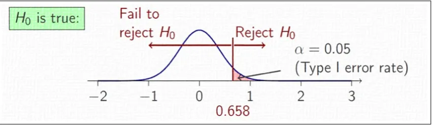
To understand whether or not H0has to be rejected, the calculated p-value is compared to a

thresholdαcommonly referred to assignificance level. This value represents the probability of making a so-called “Type I” error, which occurs with the incorrect decision of rejecting a true null-hypothesis, as in indicated in table3.

(17)

a probabilityαof making a Type I error, its correctness can be trusted with a probability of 1−α. This figure is referred to asconfidence level, and it is sometimes provided instead ofαin the literature.

H0is true H0is false

Test rejects H0 _{(False Positive)}Type I error Correct inference_{(True Positive)}

Test fails to rejects H0 Correct inference_{(False Negative)} _{(True Negative)}Type II error

Table 3.Table of truth, aka confusion matrix.

By default, SOS performs the Wilcoxon Rank-Sum test withα= 0.05, which is the most used value, unless differently specified before running the test. This results in a confidence level of 95%. To employ a differentαvalue, a better method is provided, see the online documentation, and other are also available to switch from two-sided to one-sided and decide whether or not p-values have to be shown on screen.

To conclude, once the p-value is computed and the significance levelαchosen, a final decision is made by mean of the following logic:

• if p-value≥α, the test fails at rejecting H0 : A=B and does unveil any significant difference

between A and B – the two algorithm are equivalent on P;

• if p-value<α, the test reject H0 : A=B and one can be(1−α)% confident that a significant

difference does exist between A and B.

A graphical example summarising this process is provided in figure5.

Figure 5.A graphical explanation of the hypothesis testing process for a generic one-sided test with alternative hypothesis H1: A>B andα=0.05. The area under the normal distribution, highlighted

in red, is equal toαand indicates therejection zone. Indeed, anyx>0.658 would return a p-value

(i.e. area under the distribution) lower thanα, thus rejecting H0. Conversely, for allx<0.658 the corresponding p-value would be greater thanα, thus failing to reject H0. In a two-sided equivalent scenario, the red area on the right-hand side should have a symmetric counterpart on the left-hand side. The two resulting tails, each one casting an area of 0.025 (i.e. α

2 = 0.052 , so that the total significance level is 0.05 and the corresponding confidence is 1−α=95%) would form the rejection zone.

4.2. The Holm-Bonferroni test for metaheuristic optimisation

The Holm test is a non-parametric and sequentially-rejective procedure for multiple-hypothesis testing which aims at rejecting a hypothesis at a time until no further rejection is possible [78].

(18)

The original Holm test was designed with the intent of guaranteeing a reasonably low family-wise error rate (FWER) [12,78] – an error plaguing multiple-hypothesis testing and known to increase when the number of hypotheses increases. To further improve upon this aspect and keep the FWER low even when the number of hypotheses is high, several “corrections” for obtaining more informed p-values have been proposed. The Bonferroni’s corrections are among the most popular [84].

SOS implements a simple Holm-Bonferroni test for comparing stochastic algorithms consisting of the steps in sections4.2.1to4.2.4.

4.2.1. Choosing the reference algorithm

Let us consider a generic experiment E containing NA algorithms and NP problems. When the test is run on E, SOS will display the list of available algorithms and ask the user to select the reference algorithm.

Unlike the case described in section4.1.1for the Wilcoxon Rank-Sum test, this step can change the output of the test. Indeed, in the one-to-one comparison performed with a Wilcoxon Rank-Sum test, exchanging A with B would not alter the rank distributions obtained on P. Conversely, NA−1 test statistics are computed in a Holm-Bonferroni test and these values do depend on the rank of the reference algorithm. In this light, if the goal is to test the performance of an algorithm A in E against the other algorithms, A should play the role of the reference algorithm. On the contrary, if the goal is to understand which algorithm has the best overall performance in E, it could be necessary to run the test twice. The first time, a random reference is chosen. The second time, the algorithm with the highest rank must be individuated and selected to be the reference for a second round of the test.

Once a reference algorithm is selected, value SOS proceeds with the test.

4.2.2. Assigning ranks

First, the average final fitness value must be computed with values returned by the NA algorithms after the execution of multiple runs. SOS automatically collects the text files containing the information stored inFTrendobjects and provides the NP final average values for each algorithm7_.

Then,

• for each problem in E a score equal to NA is assigned to the algorithm displaying the best average performance in terms of its objective function value, i.e. the greatest if it is a maximisation problem or the smallest if it is a minimisation one, while a score equal to NA−1 is assigned to the second-best algorithm, a score equal to NA−2 to the third-best algorithm, and so on. . . the algorithm with the worst final average fitness value gets a score equal to 1;

• for each algorithm in E the scores assigned over the NP problems are collected and averaged:

– the average score of the reference algorithm is referred to as rankR0;

– the remaining NA−1 average scores are used to sort the corresponding algorithms in descending order and constitute their ranks, which are indicated with Ri (i = 1, 2, 3, . . . , NA−1).

Ranks give us a first indication of the global performance of the algorithms on E, and their order will be automatically displayed in the form of a “league” table.

4.2.3. Zed Statistic and P-values

This test requires the use of the so-called “zed value” statistic[12], calculated with the formula

(19)

zi= _qRi−R0 NANA_6NP+1

for eachithcomparison algorithm (i=1, 2, 3, . . . , NA−1).

This allows for the determination of NA−1 probability values pi-value (i=1, 2, 3, . . . , NA−1)

through thenormalised cumulative normaldistributionszifor each comparison algorithm. 4.2.4. Sequential decision-making

When all the previous steps are completed, SOS can proceeds with a sequential decision-making process in which A is tested against each comparison algorithm, following the order obtained in section4.2.2, individually. A similar procedure to that one presented in section4.1.5for the Wilcoxon Rank-Sum test is therefore iterated NA−1 times in this step of the Hom-Bonferroni test. However, the rejection threshold requires some adjustments. In details, For eachith comparison algorithm (i=1, 2, 3, . . . , NA−1), taken in the order established in section4.2.2, the corresponding pi-value and

thresholdα/iare compared: • if p_i-value≥ α

i the test fails at rejecting the null-hypothesis H0: A=B; • if p_i-value < α

i the null-hypothesis is rejected and the rank can be used as an indicator to

establish which algorithm displayed a better performence on E.

A table displaying the outcome of the test is automatically generated. Some examples are available in section5. It is worth remarking that SOS employs a defaultα=0.05 also for this test. However, this can be changed how previously pointed out in section4.1.

4.3. Advanced Statistical Analysis

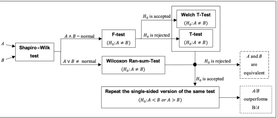
The SOS platform provides a novel advanced statistical analysis procedure, referred to as ASA procedure, for comparing couples of algorithms on a single problem. This procedure makes use of several statistical tests and it is based on simple logic, displayed on figure6, based on the fact that non-parametric tests are preferable if the assumption of normality cannot be made on the results distributions, whether parametric ones should be used if statistical evidence is found in support of such assumption. Therefore, SOS checks the results distributions of two selected algorithms, A and B, looking for such evidence and apply the most appropriate tests accordingly.

To launch this routine, the a TableAvgStdStat object must be initiated with the UseAdvancedStasticBoolean flag set equal totrue, see figure7. It must be remarked that if such flag is not activated, the Wilcoxon Rank-Sum Test is performed. It has been noted that the two tests differ when the number of runs is inferior to 100. In such a case, it is strongly recommended to use ASA for a more accurate caparison. Conversely, when a very high number of runs is available, ASA and Wilcoxon Rank-Sum are comparable. For this reason, the default number of runs performed by SOS is 100. However, this number of runs might be unpractical when facing time-consuming real-world optimisation problems. Hence, as explained in the previous sections, see figure2, SOS provides a setter method for specifing the number of runs to be performed in a given experiment. The most common values used in the literature range from 30 to 60 runs.

When the ASA procedure is activated, SOS performs the following steps:

• the Shapiro-Wilk test [85] is run on the reference algorithm A and subsequently on the comparison algorithm B with null-hypothesis H0: “results are normally distributed”;

• if both A and B are normally distributed (i.e. the Shapiro-Wilk test fails at rejecting H0both the

(20)

◦ if the variances are equivalent it is concluded that both A and B have normal distributions, which suggests the use of a two-sided T-test [87,88] with null-hypothesis H0 : A 6= Bto

make a decision according to the following logic

- if H0is rejected, A and B are two equivalent stochastic processes. The test terminates

here.

- if the test fails at rejecting if H0a one-sided T-test [87,88] is run to understand if A

outperforms B, i.e. H0: A<B is rejected, or B outperform A, i.e. H0: A>B is rejected.

The test terminates here.

◦ if variances are not equivalent, the Welch T-test [89,90] has to be used to with null-hypothesis H0: A6=B;

- if H0is rejected A and B are two equivalent stochastic processes. The test terminates

here.

- if the test fails at rejecting if H0a one-sided Welch T-test [89,90] is run to understand

if A outperforms B, i.e. H0: A <B is rejected, or B outperform A, i.e. H0: A >B is

rejected. The test terminates here.

• if at least one between A and B is not normally distributed (i.e. the Shapiro-Wilk test rejects H0

in at least one case) a non-parametric test is necessary and a two-sided Wilcoxon Rank-Sum test is performed to test H0: A6=B8and

◦ if the null-hypothesis is rejected A and B are two equivalent stochastic processes. The test terminates here.

– if the test fails at rejecting H0, a one-sided Wilcoxon Rank-Sum test is run to understand if

A outperforms B, i.e. H0: A<B is rejected, or B outperform A, i.e. H0: A>B is rejected.

The test terminates here.

A graphical scheme is in figure6.

Figure 6.ASA flow diagram.

5. Visual representation of results

With SOS, results can be displayed in several formats. After performing an experiment, raw data are located in the SOSresultsfolder, unless differently indicated, and can be processed straight away

8 _{For logistic reasons, it is more convenient to formulate the null-hypothesis as H}

(21)

or merged with those from other experiments before being processed. In theresultsfolder, data are arranged in sub-folders with self-explanatory names to be easily individuated. The main folder comes with the name of the experiment and contains a text file describing it, as explained in section2.1, as well as sub-folders whose names refer to the benchmark suite used, the specific function identifier and the dimensionality of the problem. Inside each folder, a fitness trend file is stored for each performed run. On top of the fitness values trend, these files also report full coordinates of the found near-optimal solution.

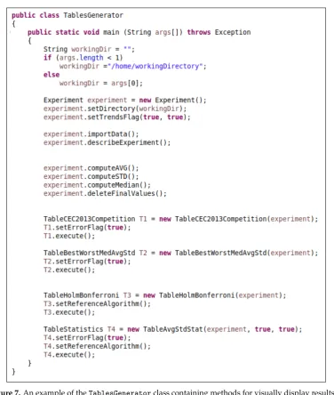
From the raw data, SOS can extrapolate information and create graphs and tables thanks to several auxiliary methods available in the platform. The classExperimentsprovides some of these routines for collecting data and transform them into more useful formats. Some of these can be seen in figure7, which depicts the main method of theTablesGeneratorclass located in the default package.

Figure 7.An example of theTablesGeneratorclass containing methods for visually display results in several different formats.

(22)

second Boolean value is alsotrue, the graph will show the fitness trend in terms of average error9, as shown in figure8, rather than average fitness. Outputs will look like the examples reported in figure8. More details regarding the preparation of fitness trends diagrams are given in appendix A. The following experiment.importData(); andexperiment.describeExperiment(); methods will start this process and describe it (in the generated log file) repetitively. If the fitness trends flag is not active, theimportData()method will collect data from the corresponding folders, process them, but will store in memory only the information required for the generation of tables without saving the average trends information into the plottable files. Once raw data are loaded in memory, SOS can be asked to extrapolate information to be displayed in tables. For example, the commands experiment.computeAVG();andexperiment.computeSTD();will lead to a table where the average fitness value (or average fitness error value if the error flag is active)±the corresponding standard deviation are shown. The commandexperiment.computeSTD(); will instead return the median fitness value (or median fitness error depending on the error flag) amongst the available runs. In the example of figure7the three methods are used but this is not compulsory. It is indeed possible to call only some of or none of them. Moreover, other methods not included in this example are also available, e.g. those for displaying the best of the wort run. If the methods are not called at all, when running a specific test, as shown in the reminder of figure7, the required one will be automatically called. Conversely, if they are called, it is suggested to useexperiment.deleteFinalValues();to free some memory by discarding the loaded final results value and keep only their average (plus standard deviation) and mean value. Before freeing the memory one may want to save the final values to plot histograms and distributions. Even if this is not common in the literature, it might be useful to do this in some cases and can be done in SOS by simply activating flags. For more technical details on SOS full capabilities, one may want to inspect the online software documentation.

At this point, the statistical tests described in section4can be launched to produce tables in PDF and LA_{TEXsource code formats. To structure compact but highly informative tables, SOS provides}

specific classes. Let us keep following the example in figure7. One can see that four classes are used to produce tables for theexperimentobject passed as an argument to the constructor. These classes are:

• TableCEC2013Competition, whose objects can produce tables displaying results according to guidelines of IEEE CEC competitions (i.e. the indications for CEC 2013 [72] competition are considered);

• TableBestWorstMedAvgStd, whose objects can produce tables displaying the worst, the best, the median and the average fitness value over the performed runs;

• TableHolmBonferroni, whose objects can produce tables displaying the “experiment’s league table”, as shown in the examples of figure9, obtained with the Hold-Bonferroni test as explained in section4.2;

• TableAvgStdStat, whose objects can produce tables displaying fitness average value±standard deviation and statistical analysis in terms of Wilcoxon Rank-Sum test, as described in section4.1, or ASA test, as described in section4.3. Examples are given in figure10.

This four classes are all extensions of the abstract classTableStatisticsfrom which they inherit several miscellaneous methods, as e.g. thesetErrorFlag()method (used to indicate the reference algorithm) if tables should display average fitness or errors values), thesetRefenceAlgorithm() method (used to indicate the reference algorithm) and theexecute()method (which implements the specific statistical test), as well as attributes, as e.g. variables to store the significance levelsα, confidence levelsδ=1−α, error and other flags, etc.

(23)

(a)

(b)

Figure 8.Example of average fitness (error) trends produced with SOS for the study in [23]. In (a), the full image with caption. In (b), a further example of an average error trend from the same study plotted in both linear and logarithmic scale. More examples from several other studies are gathered in [91].

Hence, if a new customised table must be added, this can be simply done by expending the TableStatistics superclass and make use of the auxiliary methods provided in such class to implement theexecute()where new tests can be used and new layouts for the tables can be proposed.

However, the tables produced with theTableHolmBonferroniandTableAvgStdStatclasses are the most requested for publications within the metaheuristic optimisation field when algorithms have to be compared in terms of the quality of the returned fitness values. Hence, in the vast majority of cases, these are the only two necessary kinds of tables to insert in a publication providing a comparative analysis. To further describe the informative content of these tables, let us refer to the examples reported in figures9and10.

(24)

(a)

(b)

Figure 9. Two examples ofTableHolmBonferronitables. In (a), some results from the study in [4] obtained with the non-rotated functions of the R-CEC14 benchmark suite presented in section3.1. More examples are available in the extended results files stored in the repository [92]. In (b), some results from the study in [66] obtained over the functions of the SOS implementation of the CEC 2014 [2] benchmark suite. Extended results tables for this study are available in the repository [91].

order according to their rank. As can be seen by comparing the Rank andpjcolumns, this corresponds to a descending order also for the p-values. This way, algorithms in occupying top positions are quite likely to behave similarly to the reference algorithm (i.e. the null-hypothesis is accepted) while those occupying lower positions behave worse than the reference algorithm (i.e. the null-hypothesis is rejected). Relevant information as the z-statistic values and normalised significance/confidence levels can be also added.

Conversely, figure10shows two examples of classic comparative tables obtained with the class TableAvgStdStat.At first glance, it can be noticed that the best performance (in terms of average fitness error) is highlighted in boldface. This is obtained by setting theuseBoldflag equal totrue, as in the example of figure7. Generally, the boldface option is useful as it allows for spotting the “winner” algorithm in a facilitated way. However, it can be turned off by simply settinguseBold = false.

(25)

Regardless of the emplyed statistical test, the same compact notation is adopted to report its outcome in the table:

• if the reference algorithm A (i.e. the first one in the table) is statistically equivalent to a comparison algorithm B (i.e. H0: A=B cannot be rejected), the symbol=is placed next to B;

• if the reference algorithm A statistically outperforms a comparison algorithm B, the symbol+is placed next to B;

• if the reference algorithm A is statistically outperformed by a comparison algorithm B, the symbol−is placed next to B.

(a) Wilcoxon Rank-Sum test

(b) ASA test

(26)

It is important to highlight the importance of having statistical evidence next to the average fitness error value. For example, with reference to figure10-(a), it can be noticed that despite (1+1)-CMA-ES displays the best average error value for f2, this is quite likely to be an isolated event as the=symbol next to it suggests that its general behaviour is actually equivalent to the one of the reference algorithm, i.e. RI-(1+1)-CMA-ES, from the statical point of view. Indeed, there is a very small difference between the two average error values, i.e. of about 10−14, which is mathematically in favour of the comparison algorithm but not practically insufficient to be able to state that the comparison algorithm outperforms the reference algorithm.

Supplementary Materials: Further material can be obtained from the following open access repositories

• Raw data and extended galleries of tables and fitness trend graphs generated with SOS for some of the studies mentioned in this article are available in [91,92];

• extensive galleries of images obtained with the joint use of SOS, for generating data, and the IOHprofiler in [7], for plotting them, are available in [41].

Funding:This research received no external funding.

Acknowledgments:I would like to thank Dr Olga Olga Zlydareva for making the SOS logo.

Terminology

The following terminology is used in this manuscript:

Computational budget Maximum allowed number of fitness evaluations for an Optimisation process Fitness function The objective function (from the EAs jargon, usually refers to a scalar function) Fitness The value returned by the fitness function

Fitness landscape Refers to the topology of the fitness function co-domain

Basin of attraction A set of points from which a dynamical system moves to a particular attractor Run An optimisation process during which one algorithm optimises one problem Initial guess Initial (random/passed) solution of an algorithm

Population-based A metaheuristic algorithm requiring a set of candidate solutions to function Individuals In the EA jargon this is equivalent to say candidate solution

Population The set containing the individuals

Population size Number of solutions processed by a population-based algorithm Variation operator Perturbation orator typical of EAs, such as e.g. crossover and mutation

Recombination op. Operator (from EAs) producing a new solution from 1 or more available individuals Mutation op. Operator (from EAs) perturbing a single solution

parent selection Methods for selecting candidate solutions in EAs to perform Recombination Survivor selection Method to form a new population from available individuals

(27)

Abbreviations

The following abbreviations are used in this manuscript:

CEC Congress on evolutionary computation CMA Covariance matrix adaptation

DE Differential evolution EA Evolutionary algorithm EC Evolutionary computation ES Evolution strategy FWER family-wise error rate GA Genetic algorithm

IEEE Institute of electrical and electronics engineers NFLT No free lunch theorem

PSO Particle swarm optimisation SI Swarm Intelligence

SOS Stochastic optimisation software

Appendix A. Producing the fitness trend

To save a plottable file containing the average fitness trend of an algorithm over a specific problem, SOS first fills an array of size equal to the computational budget with the values from theFTrendobject returned by the algorithm. This is done for each performed run. The initial and final fitness values are always available. However, if some intermediary fitness values are not available from the returned FTrendobject, SOS fills these gaps with the previous fitness value. This way, a monotone and complete sequence of fitness values, reproducing the optimisation trend of a single run, is available and ready to averaged with those obtained from the other runs. The resulting average fitness trend is stored in another array of equal dimension. Subsequently, the content of these arrays is downsampled to have 500 equispaced (in terms of fitness evaluation counter) elements. This results in better quality graphs as those in figure10– sometimes, having too many values does not lead to easier-to-interpret plots and it is always better to have equispaced points to avoid dense clusters followed by empty spaces in the fitness trend. However, it must be pointed out that the number of points plotted in the fitness trend can be changed, thus allowing for a higher or lower number of fitness values to be included in the graphs to adapt to specific needs.

References

1. Caraffini, F.; Kononova, A.V.; Corne, D. Infeasibility and structural bias in differential evolution.Information Sciences2019,496, 161–179. doi:10.1016/j.ins.2019.05.019.

2. Liang, J.J.; Qu, B.Y.; Suganthan, P.N. Problem definitions and evaluation criteria for the CEC 2014 special session and competition on single objective real-parameter numerical optimization. Technical report, Computational Intelligence Laboratory, Zhengzhou University, Zhengzhou China and Technical Report, Nanyang Technological University, Singapore, 2013.

3. Caraffini, F.; Neri, F.; Picinali, L. An analysis on separability for Memetic Computing automatic design. Information Sciences2014,265, 1–22. doi:10.1016/j.ins.2013.12.044.

4. Caraffini, F.; Neri, F. A study on rotation invariance in differential evolution. Swarm and Evolutionary Computation2019,50, 100436. doi:10.1016/j.swevo.2018.08.013.

5. Mittelmann, H.D.; Spellucci, P. Decision tree for optimization software.http://plato.asu.edu/guide.html, 2005.

6. Hansen, N.; Auger, A.; Mersmann, O.; Tusar, T.; Brockhoff, D. COCO: A Platform for Comparing Continuous Optimizers in a Black-Box Setting. ArXiv2016,[1603.08785].

7. Doerr, C.; Ye, F.; Horesh, N.; Wang, H.; Shir, O.M.; Bäck, T. Benchmarking discrete optimization heuristics with IOHprofiler. Applied Soft Computing2020,88, 106027. doi:10.1016/j.asoc.2019.106027.