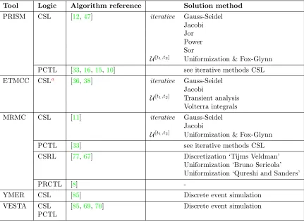
Probabilistic model checking
A comparison of tools
Masters Thesis
in Computer Science
of
H.A. Oldenkamp
born on the 23th of September 1979May, 2007
Chairman:
Prof. Dr. Ir. Joost-Pieter Katoen
Supervisors: Ivan S. Zapreev MSc Dr. David N. Jansen Dr. Mari¨elle I.A. Stoelinga
University of Twente, Faculty EEMCS,
Summary
Model checking is a technique to establish the correctness of hardware or software systems in an automated fashion. The goal of this technique is to try to predict system behaviour, or more specif-ically, to formally prove that all possible executions of the system conform to the requirements.
Probabilistic model checking focusses on proving correctness of stochastic systems (i. e. systems where probabilities play a role). A probabilistic model checker tool automates the correctness proving process. These tools can verify if a system – which is described by a model, written in a formal language – satisfies a formal specification, which is expressed using logics, such as Proba-bilistic Computation Tree Logic (PCTL). We have studied the efficiency of five probaProba-bilistic model checker tools, namely: PRISM (Sparse and Hybrid mode), MRMC, ETMCC, YMER and VESTA. We made a tool by tool comparison, analysing model check times and peak memory usage. This was achieved by using five representative case studies of fully probabilistic systems, namely; Syn-chronous Leader Election (SLE), Randomized Dining Philosophers (RDP), Birth-death process (BDP), Tandem Queuing Network (TQN) and Cyclic Server Polling System (CSP). Besides their performance, we also investigated the characteristics of each tool, comparing their implemen-tation details, range of supported probabilistic models, model specification language, property specification language and supported algorithms and data structures. During our research, we have performed nearly 15,000 individual runs. By ensuring that our experiments are automated, repeatable, verifiable, statistically significant and free from external influences, our findings are based on a solid methodology.
We have witnessed a significant difference in model check time as well as memory usage between the tools. From our experiments we learned that YMER (which is a statistical tool) is by far the best tool for verifying medium to large size models. It outperforms the other statistical model checker VESTA and all numerical tools. YMER has a remarkably consistent (low) memory usage across various model sizes. Although its performance is excellent, we found that YMER does have limitations: the range of supported models and probabilistic operators is limited and it can not provide the same level of accuracy as numerical tools. YMER may occasionally report wrong answers, but this can be expected of tools using a statistical approach, where there exists a trade-off between speed and accuracy. The benefit of statistical tools is that they scale much better (performance wise) in relation to the state-space size than the numerical tools.
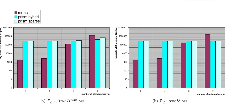
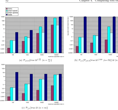
Comparing the numerical tools we conclude that MRMC has the best performance (time and memory wise) for models up to a few million states. This is especially true for steady-state and nested properties1, for other properties (i. e. bounded Until,interval Until and unbounded
Until) MRMC and PRISMSparseare rather close. On larger models, PRISMSparse (and sometimes also PRISMHybrid) performs better. The sparse engine is usually faster than the hybrid engine at the cost of substantially greater memory usage. As for ETMCC, it has the worst time and memory performance, it frequently runs out of memory in situations where the models could easily be checked by the other tools. The performance differences between the two leading numerical tools MRMC and PRISM have several causes. First of all, PRISM always construct an MTBDD (Multiterminal Binary Decision Diagram), in sparse mode the MTBDD is converted to a sparse matrix after performing some pre-computations. This may take a significant time and influence the model check time. There is no such influence for MRMC as it starts model checking on the pre-generated sparse matrix. Secondly, the MTBDD size plays a crucial role in PRISMs performance. Large MTBDDs lead to poor performance of the hybrid engine. The difference between MRMC and PRISMS is caused by the pre-computation step that is performed by PRISM on the MTBDD. The pre-computation time is included in the model check time. Finally, MRMCs performance on large models might be influenced by its high memory usage, in situations where the memory usage exceeds the systems RAM space, swapping will cause a slow down.
On the aspect of user friendliness we find PRISM the most user friendly tool. MRMC is more appropriate as a fast back-end verification engine as it has a simple input format.
1We verified two nested properties, namely for the BDP case study: P
≥1[P≥0.9[trueU≤100(n= 70)]U(n= 50)]
Preface
This master thesis project has been a challenging and educational activity. I have had the oppor-tunity to work on a project that deals with collecting, analysing and interpreting vast amounts of information, which honed my methodical and analytical capabilities. Another benefit of this project is that I gained an insight into the field of probabilistic model checking, which was a relatively new subject to me.
I would like to thank all of my supervisors for there patience and thorough feedback. I am also grateful for the information provided by Dr. Dave Parker from the University of Birmingham on the inner workings of the PRISM tool. On a final note I would like to say to my first supervisor, Ivan Zapreev:
IVAN, OQEN^ PRIZNATELEN ZA GVO NEOCENIMU POMOW^.
Glossary
BDD Binary Decision Diagram
BDP Birth-Death Process
BSCC Bottom Strongly Connected Component
CMRM Continuous Markov Reward Model
CSL Continuous Stochastic Logic
CSP Cyclic Server Polling
CSRL Continuous Stochastic Reward Logic
CTMC Continuous-Time Markov Chain
CUDD CU Decision Diagram
DMRM Discrete Markov Reward Model
DTMC Discrete-Time Markov Chain
ETMCC Erlangen-Twente Markov Chain Checker
GPL General Public License
GSMP Generalized Semi-Markov Process
GUI Graphical User Interface
J2SE Java 2 Standard Edition
JOR Jacobi Over-Relaxation
JVM Java Virtual Machine
MDP Markov Decision Process
MOVES Software Modelling and Verification
MRMC Markov Reward Model Checker
MTBDD Multi-Terminal Binary Decision Diagram
OS Operating System
OSSD On-the-fly Steady-State Detection
PCTL Probabilistic Computation Tree Logic
PEPA Performance Evaluation Process Algebra
PRCTL Probabilistic Reward Computation Tree Logic
PRISM Probabilistic Symbolic Model Checker
QuaTEx Quantative Temporal Expressions
RAM Random Access Memory
RDP Randomized Dining Philosophers
RSS Resident Set Size
RWTH Rheinisch-Westf¨alische Technische Hochschule
SLE Synchronous Leader Election
SOR Successive Over-Relaxation
State-space The set of all possible states and transitions.
STD Student’s t-Distribution
Swap The memory space (i. e. RAM) of a computer can be extended by using the hard drive as memory. This is called swap. Note that accessing swap memory typically takes a lot longer than accessing RAM.
SZ Size (memory) in physical pages
TQN Tandem Queuing Network
Contents
Glossary 7
1 Introduction 11
1.1 Approach . . . 11
2 Background on probabilistic model checking 15 2.1 Model checking . . . 15
2.2 Probabilistic model checking . . . 16
2.3 Probabilistic models . . . 17
2.3.1 Discrete-Time Markov Chains (DTMC) . . . 18
2.3.2 Continuous-Time Markov Chains (CTMC) . . . 19
2.4 Logics for checking probabilistic models . . . 21
2.4.1 Probabilistic Computation Tree Logic (PCTL) . . . 21
2.4.2 Continuous Stochastic Logic (CSL) . . . 22
2.5 Model checking Markov chains . . . 23
2.5.1 Numerical and statistical methods . . . 23
2.5.2 PCTL model checking of DTMCs . . . 24
2.5.3 CSL model checking of CTMCs . . . 25
2.5.4 Solving a system of linear equations . . . 26
2.6 State-space representation: Explicit and Symbolic . . . 27
3 Probabilistic model checker tools 29 3.1 PRISM . . . 29
3.2 ETMCC . . . 31
3.3 MRMC . . . 32
3.4 YMER . . . 34
3.5 VESTA . . . 35
3.6 Summary . . . 36
4 Comparing tool efficiency 39 4.1 Experiment setup . . . 39
4.2 Model construction . . . 43
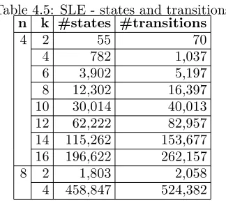
4.3 Case studies: data collection and interpretation . . . 44
4.3.1 Synchronous Leader Election . . . 45
4.3.2 Randomized Dining Philosophers . . . 48
4.3.3 Birth-death process . . . 50
4.3.4 Tandem Queuing Network. . . 54
4.3.5 Cyclic Server Polling System. . . 60
4.4 Analysis . . . 66
4.4.1 Analysis by probabilistic operator. . . 67
4.4.2 Causes of performance differences . . . 72
5 Conclusion 77
5.1 Recommendations . . . 79
5.1.1 Comparative research . . . 79
5.2 Future Work . . . 80
APPENDICES 81 A Tool settings 83 B Case studies: Model size and sample size 85 B.1 DTMC . . . 85
B.1.1 Synchronous Leader Election . . . 85
B.1.2 Randomized Dining Philosophers . . . 85
B.1.3 Birth-death process . . . 86
B.2 CTMC . . . 86
B.2.1 Tandem Queuing Network . . . 86
B.2.2 Cyclic Server Polling system . . . 87
C Model check times 91 C.1 Synchronous Leader Election . . . 91
C.2 Randomized Dining Philosophers . . . 92
C.3 Birth-death process . . . 92
C.4 Tandem Queuing Network . . . 93
C.5 Cyclic Server Polling system . . . 94
D Peak Memory consumption 97 D.1 Synchronous Leader Election . . . 97
D.2 Randomized Dining Philosophers . . . 98
D.3 Birth-death process . . . 98
D.4 Tandem Queuing Network . . . 99
D.5 Cyclic Server Polling system . . . 100
Chapter 1
Introduction
In the early days of software (and hardware) development, it was (and regularly still is) com-mon practice to write software first and (perhaps) test it later. The concept of verifying soft-ware/hardware correctness by means of testing often proved inadequate for complex systems. Experience learned that the effect of software bugs can vary from causing a slight inconvenience to disastrous effects, such as the explosion of the Ariane 5 launch system. Since the early 80’s, people have been working on a way toformally verify whether a system satisfies a certain behavioural property by means of a technique called model checking [21]. Model checking is a technique to establish the correctness of a system. In contrast to testing, model checking looks atall possible behaviours of a system. While testing can only find errors, formal verification by means of model checking can also prove their absence. It enables expressing properties to which the answer is “yes” or “no”, such as: it is never the case that traffic lights “A” and “B” are green simultaneously. While formal verification focuses on the absolute correctness of systems, in practice such inflexi-ble demands are hard, or even impossiinflexi-ble, to guarantee. Instead, systems are subject to various phenomena of stochastic nature, such as message loss or garbling, unpredictable environments, faults, and delays. Correctness thus is of a less absolute nature. Accordingly, instead of checking whether system failures are impossible, a more realistic aim is to establish, for instance, whether “the chance of failure is at most 0.01%”. Such properties can be checked using probabilistic model checking. There are many software tools available that automate the process of probabilistic model checking. Such tools accept a system model description (“the possible behaviour”), a specification of the property to be considered (the “desirable behaviour”), and then systematically check the validity of the property on the given model.
We are interested in the performance difference between available probabilistic model checker tools. We desire an in-depth analysis of the difference in speed (i. e. how much computation time does the tool require to verify a particular model and property) and memory usage (i. e. the maximum amount of memory consumed by the tool). In addition, we are interested in the overall differences amongst the tools, such as their variety of supported probabilistic models and logical operators for property specification. This thesis sets out to compare several model checkers for probabilistic systems (henceforth called tools), by means of an empirical study, and attempts to observe and explain relevant phenomena.
1.1
Approach
inter-12 Chapter 1. Introduction
est to compare. In the initial phase we investigated the general characteristics of each tool and compared their implementation details, range of supported probabilistic models, model specifi-cation language, property specifispecifi-cation language (i. e. temporal logic operators) and supported algorithms & data structures. This was accomplished by investigating available documentation and publications related to the tools and naturally by using the tools themselves. The core of the project involved an in-depth study into the performance differences between each of the tools. We therefore constructed a test environment to gather and analyse data related to:
1. speed - the computation time required to verify a particular model and property 2. memory usage - the peak memory consumed by the tool during its execution
Using five representative case studies taken from the literature on performance evaluation and probabilistic model checking we performed several experiments. For each case study we generated equivalent1models written in the model description language of each individual tool. We
constructed a set of properties expressed in the temporal logic PCTL (Probabilistic Computation Tree Logic) or CSL (Continuous Stochastic Logic) and arranged for the size of the model to be adjustable. We then collected performance data by letting each tool verify the properties on all the model sizes.
In order to gather reliable data, we created an isolated test environment, meaning; we made sure the conditions for each experiment were the same except for the independent2 variables (i. e. the
ones we want to manipulate, namely the model size and property). We used a standard Personal Computer that was designated to this project only, such that others could not inadvertently change the environment. All the data, such as tool installation files, input models and result files were stored on the local hard drive, as to avoid influence in performance measurements due to network traffic issues. The tools were considered as a “black box”, meaning we made external measurements. This ensured a uniform method of collecting performance data, independent of the tools implementation. We did not build any measurement constructions into the source code of the tools, since this might influence their performance, in addition, this would require the availability of the source code of each tool. The verification parameters of each tool were set to corresponding levels. For example, the error bound , which is used in solving a system of linear equations, is set to 10−6 for all non-statistical tools.
Automation. Because we created multiple properties and model sizes per case study, and had
to verify each combination using the five tools, automation became a necessity (we performed nearly 15,000 individual runs). All experiments and measurements were automated by means of Linux shell scripts. This enabled us to easily repeat experiments many times and collect data in a uniform style. An experiment consisted of verifying one property on one particular model size using one of the model checker tools. The tools were restarted before each experiment; this prevents features such as caching to influence the results. Each experiment was repeated 20 times, after which we calculated the sample mean and standard deviation of data such as elapsed time. The number of runs was limited to 3 in stead of 20 whenever the total time of a single run exceeded 30 minutes, this prevented experiments from consuming excessive amounts of time, but resulted in a less accurate standard deviation. To counter this effect we used the student’s t-distribution [26], which takes the number of samples into account. The raw data produced by the tools was processed automatically by means of shell scripts and a Java application that we designed to perform the necessary calculations and generate results for easy display in LATEX3.
1With equivalent models we mean that they model the same system and reflect identical (possible) behaviour. 2Anindependent variable is selected and manipulated by the experimenter to observe its effect on the dependent
variable (i. e. the variable that is observed and measured) [31].
3LA
Chapter 1. Introduction 13
Organisation of the thesis. Chapter 2 presents the necessary background information on
(probabilistic) model checking, including the different probabilistic models such as Discrete-Time Markov Chains and Continuous-Time Markov Chains and the logics PCTL and CSL for property specification. Chapter3offers a tool by tool overview ranging from general background information to supported logical operators, algorithms and data structures. In Chapter4we perform a series of experiments on five probabilistic model checker tools to measure and compare their efficiency. We utilize five well known case studies and compare the performance results of each tool. We measure and analyse the time and peak memory usage required by each tool (to verify a specific PCTL/CSL property). Finally, Chapter5concludes the thesis.
Chapter 2
Background on probabilistic
model checking
This chapter gives an introduction to (probabilistic) model checking, it elaborates the basic con-cepts relevant for this thesis, starting with model checking in general and moving on to probabilistic model checking, probabilistic models and logics for checking probabilistic models.
2.1
Model checking
When designing systems (hardware or software) it is important to know whether or not your system will operate as expected/required. For instance you do not want to find out after implementation and delivery of your nuclear power plant control system that it is not as safe as was expected. There are several techniques available that can be used to verify the functional correctness of a system. Examples of such techniques are: theorem proving, simulation/testing and model checking. This thesis focuses on the last technique, namely formal verification by means of model checking [21]. The goal of this technique is to try to predict system behaviour, or more specifically, to formally prove that all possible executions of the system conform to the requirements. Typical problems that are addressed are [38]:
• Safety [6]: e. g. does a given mutual exclusion algorithm guarantee mutual exclusion?
• Liveness [6]: e. g. will a packet transferred via a routing protocol eventually arrive at the correct destination?
• Fairness [29]: e. g. will a repeated attempt to carry out a transaction be eventually granted?
As the name suggests, model checking is performed on a model of a system. The model is usually generated from a high level system description, such as process algebra or Petri net. Typically, these generated models are non-deterministic finite-state automata1. These automata
(i. e. transition systems) describe the possible system behaviour. They can be seen as directed graphs consisting of a finite set of states (nodes) labelled with atomic propositions and state transitions (edges) that show how the system can change from one state to another. The atomic propositions represent the basic properties that hold in each state. Once the system is represented by a model we can check if the model satisfies a formal specification (i. e. if it has certain properties). The properties that are checked against the system model are expressed using logics, such as LTL (Linear Time Logic) or CTL (Computation Tree Logic). These logics can express properties on states or paths in the automata. Once a model and property have been formulated the model checking process will perform a systematic state-space exploration to verify if the property holds. This form of traditional model checking focuses on delivering a 100% accurate guarantee whether or not a property holds in a certain model. There are many cases where giving an absolute guarantee
16 Chapter 2. Background on probabilistic model checking
is not feasible or even impossible. Examples are communication protocols, such as Bluetooth or IEEE 802.11 Wireless LAN, that have to deal with a certain probability of message loss. This is where probabilistic model checking can be utilized.
2.2
Probabilistic model checking
Probabilistic model checking is an automatic formal verification technique for the analysis of systems which exhibit stochastic behaviour [41]. The technique is similar to model checking as discussed earlier. The major difference is that a probabilistic model contains additional informa-tion on likelihood or timing of transiinforma-tions between states, or to be more specific, it can model stochastic behaviour. Probabilistic model checking refers to a range of techniques for calculating the probability of the occurrence of certain events during the execution of the system, and can be useful to establish properties such as “shutdown occurs with probability at most 0.01” and “the video frame will be delivered within 5ms with probability at least 0.97” [50]. Applications range from areas such as randomized distributed algorithms to planning and AI, security [60], and even biological process modelling [55] or quantum computing. An overview of the probabilistic model checking procedure is given in Figure2.1. It shows that a probabilistic model checker takes as input a property and a model and delivers the result “Yes” or “No” (i. e. whether or not the property is satisfied) or some probability. The following sections elaborate on the input of the model checker tools, namely the model types and logics. But first an example is introduced, that is used throughout this chapter.
probabilistic model checker e.g. PRISM, MRMC probabilistic
property e.g. PCTL, CSL (logics)
probabilistic model
e.g. DTMC, CTMC
result yes / no / probability
Figure 2.1: Probabilistic model checking overview
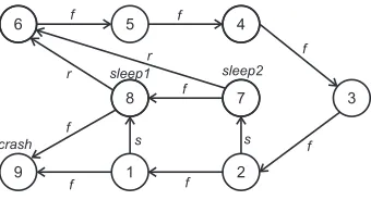
The Hubble space telescope example. This example (an adaptation from [38]) models the
failure behaviour of the Hubble space telescope2. We start by describing the real system, which
consists of parts that can possibly fail. Once the system is understood, we will model its failure behaviour, so that we may predict its behaviour and ask question such as: “What is the probability that the system will operate without failure for the next 10 years?”
System. The system has a steering unit with six gyroscopes, which are used to aim the telescope.
Redundancy is an important issue when designing systems such as the space telescope, since it is obvious that performing repairs is not trivial. This is why the telescope is designed in such a way that it will still function with full accuracy when only three of its six gyroscopes are operational. With less than three gyroscopes the telescope turns into sleep mode, meaning repairs are necessary3. If none of the gyroscopes are operational the telescope will crash. No repair
mission will be undertaken, as long as there are more than two gyroscopes operational.
Model. The model of the system that has just been described is depicted in Figure 2.2. The
model has a total of nine states. Each state has a number and label (shown respectively inside and
Chapter 2. Background on probabilistic model checking 17
outside side the state symbol). States 1 through 6 are not labelled explicitly; their labels equal their state number, which represents the number of operational gyroscopes. An edge labelled f
represent a failure event of a gyroscope,r means a repair mission has been undertaken successfully andsmeans the telescope is going to sleep. States 7, 8, and 9 are labelledsleep2,sleep1 andcrash. State 6 is considered the initial state where all gyroscopes are operational; this is also the state of the telescope after a successful repair mission. The state with labelcrashis a terminating state4. We now have a model of our system that shows its possible behaviour. Later on we expand this model by adding probabilities and rates.
6 5
Figure 2.2: State transition system of the Hubble space telescope
2.3
Probabilistic models
In order to model check a system that exhibits stochastic behaviour we will first need to build a formal probabilistic model of that system. There are several commonly used probabilistic model representations for stochastic system, for example:
• Discrete-Time Markov Chains (DTMC)
• Continuous-Time Markov Chains (CTMC)
• Markov Decision Process (MDP)
• Stochastic Petri nets
• Bayesian networks
These models usually form a combination of probability theory and graph theory. They consist of states, transitions, and arcs that connect them. From now on we will focus on Markov chains. These particular models are used by all probabilistic model checker tools studied in this thesis. A Markov chain should be considered as a transition system, where we can move from one state to another and the choice of which state to go to depends on some probability distribution. Moving from one state to another is referred to as “making a transition”. A more formal definition will be presented later on. We will only deal with Markov chains that have a finite or countable set of states, if this condition is not met, we speak of a Markov process5 [61]. A Markov chain has
a very specific characteristic, namely that it retains no memory of earlier transitions. This is called the Markov property. It means that only the current state of the process can influence the probability of next transitions. We consider two different types of Markov chains, which are frequently supported by probabilistic model checker tools:
1. DTMC - Discrete-Time Markov Chain 2. CTMC - Continuous-Time Markov Chain
The Markov chains discussed here are considered time-homogeneous (i. e. the transition matrix, containing the probabilities or rates, remains constant). The meaning of transition matrix will become clear in the next sections, where a brief explanation is given of DTMCs and CTMCs. For a more elaborate treatment see [74].
4A terminating state, also called absorbing state, is a state that once entered cannot be exited.
5When a Markov process has adiscretestate-space (set of all possible states and transitions) we call it a Markov
18 Chapter 2. Background on probabilistic model checking
2.3.1
Discrete-Time Markov Chains (DTMC)
A DTMC is a transition system that defines the probability of moving from one state to another.
Definition 2.1 (labelled DTMC). A labelled DTMC is a quadruple< S, s, P, L >where:
• S is a finite set of states,
atomic propositionsa∈AP that are valid ins. (adapted from [33])
According to [49], DTMCs are stochastic models of systems with countable state-space that change their states at times n= 0,1,2, . . .and have the following property: if the system enters statesat timen, it stays there for exactly one unit of time and then jumps to states0at timen+ 1
with probabilityP(s, s0), regardless of its history up to and including time n−1. The definition
shows that states are labelled with atomic propositions, they indicate for instance the status of the system (e. g. waiting, sending). The system can change state according to a probability distribution given by the transition probability matrix. A transition from states to s0 can only
take place ifP(s, s0)>0. IfP(s, s0) = 0, no such transition is possible. The system can occupy the same state before and after the transition, since according to definition2.1self-loops are allowed. A sequence of states and transitions forms a path, where a path is defined as a finite or infinite sequence s0
We represent a DTMC as a transition diagram, where states are depicted by circles, state labels by text outside the circle and transitions with non-zero probabilities by arrows labelled with their probabilities. Figure2.3 shows the DTMC model and matrixP of the Hubble space telescope (first introduced on page16). The number of states and transitions have remained the same, only now the transitions are assigned with probability values. It shows that as long as there are more than two gyroscopes operational the next gyroscope will fail with probability 1. This is represented by the states labelled 6, 5, 4 and 3 with outgoing transitions that have probability 1. In the situation where two gyroscopes are operational, the system can either go to the sleep
mode with probability 0.998 or one of the remaining gyroscopes may fail with probability 0.002, which is depicted by the outgoing transitions of state 2. Each possible state transition with its corresponding probability is shown in the transition system and probability matrix in Figure2.3.
6 5
Chapter 2. Background on probabilistic model checking 19
2.3.2
Continuous-Time Markov Chains (CTMC)
A CTMC can be seen as an extension of the DTMC. The difference is that a DTMC models discrete time steps and a CTMC allows the modelling of real (continuous) time. This means that state changes in a CTMC can occur at any arbitrary time, as opposed to fixed timen= 0,1,2, . . .
in a DTMC. The memoryless property still applies, meaning that the probability of moving to a future state depends only on the current state. CTMCs are often used for analysing performance and dependability of systems. Two examples of practical applications of CTMC models are; determining the mean time between failures in safety-critical systems and identifying bottlenecks in high speed communication networks. A labelled CTMC is defined as follows (adapted from [11]):
Definition 2.2 (labelled CTMC). A labelled CTMC is a quadruple< S, s, R, L > where:
• S is a finite set of states,
• s∈S is the initial state,
• R:S×S→R≥0 is the rate matrix, whereR(s, s0) is the rate of moving from statestos0,
• L : S → 2AP is the labelling function, which assigns to each state s
∈ S the set L(s) of atomic propositionsa∈AP that are valid ins.
Similar to a DTMC, the definition contains a set of states S, the labelling function L and an initial state. Instead of the probability matrixP a CTMC has a rate matrixR, which gives ratesR(s, s0) at which transitions occur between each pair of states s, s0. If R(s, s0) = 0 then no
transition from statestos0 is possible, because it has zero probability. Otherwise, ifR(s, s0)>0
and stateshas only a single possible successor states0, then 1−e−R(s,s0)·t
denotes the probability of moving from state s to s0 within t time units. In the case where state s has more than one successor, i. e.R(s, s0)>0 for more than one states0, we have to deal with competition between the outgoing transitions ofs. This can be explained as follows, suppose we have a state s with multiple outgoing transitions, as soon as we enter state s we start a countdown clock for each outgoing transition (depending on its specified rate). The transition of which the clock finishes first wins. This situation is known as the race condition. To account for the race condition we need to look at the total rate of the outgoing transitions of states, known as the exit rate:
E(s) = X
s0∈S
R(s, s0) (2.1)
The probability of moving from (a non terminating) state s to state s0 within t time units is specified as:
P(s, s0, t) =R(s, s
0)
E(s) ·(1−e
−E(s)·t) (2.2)
By determining the so calledembedded DTMC of a CTMC we can look at the pure probabilistic behaviour (i. e. ignore the time spent in any state). The probabilityP(s, s0) of moving from state sto s0 is determined by the probability that the delay of going from states tos0 finishes before
the delays of other outgoing edges froms, formally:
P(s, s0) =
(R(s,s0)
E(s) ifE(s)6= 0
0 otherwise (2.3)
20 Chapter 2. Background on probabilistic model checking
Figure2.4shows a CTMC model of the Hubble space telescope, which was introduced on page
16. We have previously seen the DTMC model, introduced in Section 2.3.1, the CMTC model takes into account the life span of a gyroscope and other time dependent events. It models the real-time probabilistic behaviour of the failure and repair of the gyroscopes. The model is based on the following assumptions:
• each gyroscope has an average lifetime of 10 years,
• the average preparation time of a repair mission is two months,
• it takes about 1/100 year (circa 3.5 days) to turn the telescope into sleep-mode,
• the base time scale is one year.
6 5
Figure 2.4: CTMC of the Hubble space telescope
State six of the model corresponds to the system state where all six gyroscopes are operational and any one of them may fail. Since each gyroscope fails with a rate of 101 (because the lifespan is 10 years and the base time scale is one year), the outgoing rate of state six is 6·101 = 0.6 (because any one of the six gyroscopes may fail). The relation between the CTMC and the embedded DTMC of the Hubble space telescope is given by equation 2.3. For example the probability of moving from state 2 to 7 is: P(2,7) = RE(2(2),7) = 100
Chapter 2. Background on probabilistic model checking 21
2.4
Logics for checking probabilistic models
Once the system is represented by a model we want to check if the model satisfies a formal spec-ification (i. e. if it has certain properties). These properties can be expressed in a formal manner using logics. These logics enable us to reason about qualitative6 or quantitative7 properties of
probabilistic systems. This section discusses two temporal logics, namely Probabilistic Compu-tation Tree Logic (PCTL) [33] and Continuous Stochastic Logic (CSL) [11], which are used for verification of DTMCs and CTMCs respectively.
2.4.1
Probabilistic Computation Tree Logic (PCTL)
Probabilistic Computation Tree Logic (PCTL) was first introduced by Hansson and Jonsson [33] as an extension of the temporal logic CTL [20] with discrete time and probabilities. PCTL allows expressing properties such as: “the probability of reaching a certain goalψwithin a specified number of steps k, via paths through a set of allowed states φ, is at least/at most some probability value”. PCTL can express properties on states (state formula) or paths (path formula) in the DTMC.
Definition 2.3(PCTL syntax). Letp∈[0,1] be a real number, andki∈Nand./∈ {<, >,≤,≥}
a comparison operator. The syntax of PCTL formulas over a set of atomic propositions AP is defined inductively as follows:
• true is a state-formula,
• Each atomic propositiona∈AP is a state formula,
• Ifφandψ are state formulas, then so are¬φandφ∧ψ,
• Ifφandψ are state formulas, thenX φandφU ψ andφU[k1,k2] ψare path formulas8, • Ifπis a path formula, then P./p(π) is a state formula.
The boolean operators ¬ and ∧ have their usual meaning, they can be used to derive the operators∨ and =⇒. The path formulas involve the next operatorX and the unboundedU or boundedU[k1,k2] until. The semantics of the next and unbounded until are equivalent to that of
CTL, whereas the bounded untilφU[k1,k2]
ψstates that “ψis satisfied in one of the firstk0 states, wherek0
∈[k1, k2] and at all preceding states [0, k0)φholds, with k1≥0 andk2<∞. The state formulaP./p(π) asserts that the probability measure of paths satisfyingπmeets the bound./ p.
We use a satisfaction relation |=M to define the truth of PCTL formulas, for states or path π in a DTMC M= (S, s, P, L). Intuitively s|=M φ means that formulaφ is true at states in
DTMCM, the same applies for path formulas.
Definition 2.4(PCTL semantics). Letp∈[0,1] be a real number,ki∈N, and./∈ {<, >,≤,≥}
6Qualitative properties assert that a certain eventφholds with probability 0 or 1 [10].
7Quantitative properties guarantee that the probability for a certain eventφmeets given lower or upper bounds
[10].
22 Chapter 2. Background on probabilistic model checking
With the PCTL syntax en semantics established, we can now for instance define the following property on the Hubble space telescope DTMC:
“The probability that the telescope eventually crashes without ever having only one operational gyroscope left is at most 10−4.”
which is expressed in PCTL as:
P≤0.001(¬“1”U “crash”)
2.4.2
Continuous Stochastic Logic (CSL)
Continuous Stochastic Logic (CSL) was originally developed by Aziz et al. [9] and later extended by Baier et al. [14]. It is based on the temporal logics CTL [20] and PCTL. It provides means to express properties on CTMCs that refer to steady-state9and transient10behaviour. CSL resembles
PCTL, in fact it extends PCTL, however the difference lies in the time domain. PCTL is restricted to step intervals of natural numbersN, whereas CSL allows real numbers greater than or equal to zeroR≥0.
Definition 2.5 (CSL syntax, adapted from [11]). Let p ∈ [0,1] be a real number, I ⊆ R≥0 a
non-empty interval and ./∈ {<, >,≤,≥} a comparison operator. The syntax of CSL formulas over a set of atomic propositions AP is defined as follows:
• true is a state-formula,
• Each atomic propositiona∈AP is a state formula,
• Ifφandψ are state formula, then so are¬φandφ∧ψ,
• Ifφis a state formula, then so isS./p(φ),
• If Ψ is a path formula, thenP./p(Ψ) is a state formula,
• Ifφandψ are state formulas, thenXI φandφ
U ψ andφUI ψare path formulas.
The state formulas do not differ from those used in PCTL, except for the steady-stateS./p(φ)
which corresponds to the long-run operatorL./p(φ). It asserts that the probability of being in a
φstate on the long run, meets the bound./ p. The path formulaXI φasserts that a transition is
made to aφstate at some time pointt∈I. FormulaφUI ψstates thatψis satisfied at some time
instant t, within the interval I and at all preceding time instants [0, t)φ holds. The unbounded until operatorU is another notion for assertingφU[0,∞] ψ. We use a satisfaction relation|=
Mto
define the truth of CSL formulas, for statesand pathπin a CTMCM= (S, s, R, L).
Definition 2.6(CSL semantics). Letp∈[0,1] be a real number, andt∈Rand./∈ {<, >,≤,≥}
a comparison operator. Also letπ[i] =si be the ith state along the pathπ. Letδ(π, i) =ti be
the time spent in state si, and let π@t denote the state occupied in pathπ at time t. (Similar
definitions can be found in [14, 11]) The satisfaction relation|=M, wheres is a state, π a path
andMa CTMC, is defined by:
s|=Mtrue for all states,
s|=Ma iffa is an atomic proposition valid in s,a∈Label(s),
s|=M¬φ iffs6|=Mφ,
s|=Mφ∧ψ iffs|=Mφ∧s|=Mψ,
s|=MS./p(φ) iff limt→∞ P rs{π∈P athM(s)|π@t|=Mφ}, s|=MP./p(Ψ) iffP rs{π∈P athM(s)|π|=MΨ}./ p,
π|=MXIφ iffπ[1] is defined andπ[1]|=Mφ ∧ δ(π,0)∈I, π|=MφUI ψ iff∃t∈I.(π@t|=Mψ ∧ (∀t0 ∈[0, t).π@t0|=Mφ)).
Chapter 2. Background on probabilistic model checking 23
Similar to PCTL, we can use CSL to formulate properties on the Hubble telescope CTMC. For instance, since the telescope is expected to last at least 10 years, it is interesting to formulate properties such as:
“The probability that the system will crash within the next 10 years is at most 2%.”
which is expressed in CSL as:
P≤0.02(trueU≤10“crash”)
2.5
Model checking Markov chains
Once a model and properties have been formulated, a model checker can verify whether of not the properties hold in the model. The verification amounts to showing that the logical expression evaluates to true when interpreted over the model. To be more formal: in order to check if state
s satisfies formulaφwe need to recursively compute the setSat(φ) ={s∈S | s|=φ} of states that satisfy φ and check if s is a member of that set. There are several different methods and algorithms available for model checking. The purpose of this section is to briefly cover the basics of solution methods of Markov Chains that are used by the tools discussed in this thesis.
2.5.1
Numerical and statistical methods
There are two primary approaches in analysing stochastic behaviour of a system: numerical and
statistical. The numerical approach is divided into symbolic [57] and numerical [74] methods. Model checking tools have to deal with the fact of rapidly increasing numbers of states and transition when generating a state-space of concurrent systems.
Symbolic algorithms try to cope with this problem, known as the state-space explosion, by
avoiding ever building the state-space as a set of nodes and transitions; instead, they represent the graph implicitly using a more compact data structure. The state-space can be represented using binary decision diagrams (see the work of Ken McMillan [57]) or more recently Multi-Terminal Binary Decision Diagram [47,24].
Numerical algorithms offer a range of methods for solving a system of linear equations, which is
needed for solving formulas containing theU operator. The advantage of using numerical methods is their high accuracy, but the drawback is that they require a large amount of memory (caused by the state-space explosion problem).
Statistical methods use simulation and sampling. So instead of building a complete state-space
24 Chapter 2. Background on probabilistic model checking
to increase. In case of a fixed number of samples, the sample collection will stop when the prede-termined maximum is reached and an answer is given based on the collected samples so far.
Further details on the differences between the aforementioned methods can be found in [84].
2.5.2
PCTL model checking of DTMCs
In this section we present an insight into the theory of PCTL model checking. This subject has been extensively discussed in for instance [33, 10, 19]. It is known from [33] that PCTL model checking on Markov chains can be done in polynomial time in the size of the system and in linear time on the size of the formula. Given a PCTL formula φ, the model checking process generally starts with building the parse tree ofφ, whose nodes represent subformulas ofφ. As stated earlier, the intent is to compute the satisfaction set Sat(φ), whereSat(φ) = {s ∈ S | s |= φ}. This is achieved by processing the subformulas in the parse tree in a bottum-up manner. The processing of leaf nodes, where the formula is either true or some atomic proposition, is straightforward. The same holds for boolean connectives, for instance Sat(Φ∧ψ) =Sat(Φ)∩Sat(ψ). Below we present an outline of the actions involved in model checking the different PCTL operators. When illustrating model checking algorithm complexities, we use the term|S|to denote the number of states in a DTMC and|E|to denote the number of transitions with non-zero probability.
PCTL Next. Calculations for the PCTL Next formula are somewhat trivial, they involve a
single matrix-vector multiplication.
PCTL Bounded Until. The calculations forU≤k amount to performing some graph analysis
and k matrix-vector multiplications11. According to [33], the number of required arithmetical
operations for bounded until formulas with a finite time boundkis at mostO(kmax×(|S|+|E|)×
|φ|) orO(|S|3× |φ|), depending on the algorithm, wherek
max is the maximum time parameter in
a formula, and|φ| is the size of the formula.
PCTL Unbounded Until. The unbounded until cannot be computed by the bounded until
method, since this would require infinitely many matrix-vector multiplications (recall thatU can be denoted as U≤∞). The technique, however, is quite similar. The algorithm will first perform
some precomputations in time O(|S|+|E|)[19], using general graph traversal algorithms or BDD fixed point computation [24]. In case the probability boundpin P./p is either 0 or 1, no further
computations are necessary. For the remaining situations (i.e. 0< p <1 ), we require solving a system of linear equations by means of numerical computations. A system of linear equations can be solved in polynomial time using direct methods (e.g., Gaussian elimination or LU decomposi-tion) or iterative methods like the Jacobi- or the Gauss-Seidel-method [74]. For large probability matrices, the iterative methods perform better. More information on algorithms for solving a system of linear equations is presented in Section2.5.4.
PCTL Long Run. TheLoperator shows the behaviour of the system in the long run. Initially,
a graph analysis is carried out to find all Bottom Strongly Connected Components (BSCC)12,
which takesO(|S|+|E|) [75] time. Then for each BSCC a system of linear equations is solved, which can be done in polynomial time. Finally, the probability of reaching each BSCC is computed, which amount to solvingP=?[trueU BSCCi]. The worst case time complexity for model checking
the long run property isO(|S|3).
11For largek, the number of multiplications might be smaller if on-the-fly steady-state detection [59,48] is applied. 12A BSCC [75] is a maximal subset (i. e. subgraph) of a graph, that once entered, cannot be exited and any two
Chapter 2. Background on probabilistic model checking 25
2.5.3
CSL model checking of CTMCs
As for PCTL, model checking CSL [11, 9, 47] proceeds by recursively computing the satisfaction sets. For CSL formulas without a time bound, the problem reduces to probabilistic model checking of DTMCs. Baier et al. [12] demonstrated that CSL model checking of time-bounded formulas can be reduced to transient analysis (in particular uniformization [45]) of CTMCs. The CSL model checking algorithms (as presented in [11]) are polynomial in the size of the model and linear in the length of the formula.
CSL Next. To determine if statessatisfiesP./p[X[t1,t2]φ], we require computing the setSat(φ)
and a single multiplication of the matrix P with a vectorb. This vector is defined as:
b(s) =
(
e−E(s)·t1−e−E(s)·t2 ifs∈Sat(φ)
0 otherwise (2.4)
CSL Bounded Until. Model checking the UI operator involves matrix–vector multiplications
and transient analysis. It requires computations on the probability matrix obtained by uniformiza-tion [45] of the CTMC. Computauniformiza-tions for the bounded until can be performed with worst case time complicity of O(|E| ·q·t2) [11], where q is the uniformization rate13, and t
2 is the upper bound of intervalI. In practice, there are some efficiency improvements possible. For instance, for larget2 the number of required computations can be reduced by applying on-the-fly steady-state detection [59, 48]. Without going into detail, if desired see [11], we like to point out that there exists a difference between the number of required computations for t1 = 0 and 0 < t1 ≤t2 in
Ut1,t2, where the latter situation is computationally more intensive.
CSL Steady-state. Computing whether s |= S./p(φ) amounts to solving a system of linear
equations (in polynomial time) combined with graph analysis methods, namely a search for all bottom strongly connected components (BSCC), which takes O(|S|+|E|) [75] time. A steady-state analysis is performed for each BSCC, after which the probabilities of reaching the individual BSCCs are computed. According to [11], steady-state analysis can be performed with a worst case time complexity ofO(N3).
Table2.1shows an overview of the worst case time complexities of algorithms for model checking CSL. These results are based on using a sparse storage structure (see Section 2.6), Gaussian elimination for solving linear equations systems and uniformization for transient analysis.
Table 2.1: From [11], Algorithms for Model Checking CSL and their (worst case) time complexity.
Operator Algorithm(s) Time complexity
S./p[Φ] BSCC detection + steady-state analysis
per BSCC + computing probability of reaching a BSCC
|E|= the number of transitions with non-zero probability
q = the uniformization rate (usually maximum entry ofE)
26 Chapter 2. Background on probabilistic model checking
2.5.4
Solving a system of linear equations
The previous sections have shown that model checking certain formulas, such asS./p(φ), involves
solving a system of linear equations. These equations take the form of Ax=b. In general there are two methods to solve a system of linear equations:
• direct methods
• iterative methods
Direct methods
Direct methods, such as Gaussian elimination [74], compute the solution of a system of linear equations in a fixed number of operations. Direct methods are only recommend when dealing with relative small models (not exceeding the order of thousands of states). The computational effort is in the order ofN3, whereNis the number of states. Although they are highly reliable, the disadvantage of methods such as Gaussian elimination is that during computation the coefficient matrix must be updated at each step of the algorithm. Because the elements in the matrix are constantly updated (in particular the zero elements) it is difficult to organize a compact storage scheme, resulting in high memory consumption. For this reason most model checker tools apply iterative methods.
Iterative methods
Iterative methods do not alter the form of the matrix and thus allow the use of compact storage schemes. For iterative methods it is not known in advance how many computations are required to achieve an accurate answer. They will perform a series of matrix-vector multiplications until the difference between iterations is less than some value. This is explained by means of an example of the Power method. The example is an abridged version taken from [74]. Suppose we have a discrete-time Markov chainMwith probability matrix
P = mediately after the first transition, the system will be either in state 2, with probability .8 or in state 3, with probability .2. The vector denoting the probability distribution after one step is thusα(1) = (0, .8, .2). This result may be obtained by the matrix-vector multiplication α(0)P. Likewise we can obtain the probability distribution after two steps:
α(2)=α(1)P= (0, .8, .2)
Thus, for any integerk, the state of the system afterktransitions is obtained by
α(k)=α(0)Pk
When the Markov chain is finite, aperiodic14 and irreducible15, also known as ergodic16, (as in
the current example), the vectorsα(k) converge to the stationary probability vectorαregardless of the choice of the initial vector. We have
lim
k→∞α
(k)=α
14A statesis periodic with periodj, if on leaving statesa return is possible only in a number of transitions that
is a multiple of the integerj >1. A state whose period is 1 is said to be aperiodic. A Markov chain is aperiodic if its states are aperiodic.
15A Markov chain is irreducible if every state can be reached from every other state.
16An ergodic Markov chain is aperiodic, irreducible, and recurrent nonnull, where a Markov chain with a finite
Chapter 2. Background on probabilistic model checking 27
After a certain (beforehand unknown) number of iterations, an equilibrium will have been reached, meaning we will no longer observe a noticeable difference in the results of the multiplications. The difference between the results of the kth and (k−1)th iteration is denoted . We usually stop
when is in the order of 10−6. The answer remains an approximation, where the accuracy depends on the desiredvalue. The Power method, as described in the example, can be used to obtain the solution for so called eigenproblems (αP =α). This method is guaranteed to converge in theory, but it is often extremely slow. There are several other iterative methods, such as Jacobi, Gauss-Seidel, JOR, and SOR, which are used to obtain the solution of a system of linear equations, such as (αQ = 0). Where Qis the matrix of transition rates, known as infinitesimal generator matrix [49,74,11]. The Jacobi and Gauss-Seidel17methods are very similar to the Power
method. The difference is that they use a different iteration matrix. Both methods do not have guaranteed convergence. In practice, the Jacobi method is usually faster than the Power method and Gauss-Seidel typically converges faster and consumes less memory than Jacobi. It is possible to improve the rate of convergence of both Jacobi and Gauss-Seidel by applying a technique called relaxation; this yields in respectively the JOR (Jacobi Over-Relaxation) and SOR (Successive Over-Relaxation) methods. These methods use a relaxation parameter ω, which (when chosen correctly) can considerably improve the convergence rate over that of Jacobi and Gauss-Seidel. The problem, however, is that the optimal value of ω depends on the problem being solved and may vary as the iteration process converges, for details see [87]. Additional information regarding the theory behind aforementioned methods can be found in [74], for complexity see [17].
2.6
State-space representation: Explicit and Symbolic
The definitions of Markov chains in Section 2.3have shown that a model representation consists of states, transitions and probabilities or rates. These representations tend to grow extremely large due to the state-space explosion problem. This is caused by the fact that a system is usually composed of a number of concurrent sub-systems. Interleaving these sub-systems to form the overall state-space results in a state-space size that is often exponential in the number of sub-systems. Systems containing several million states and transitions are not out of the ordinary. This is why it is important to use data structures that minimise the computational space and time requirements for model checking large systems. There are two well-known methods applied in state-space storage, namelyexplicit andsymbolic.
Explicit. In explicit state-space representation each state and transition is individually stored
using data structures such as a sparse matrix [65]. A sparse matrix is a matrix (i. e. array-based data structure), usually very large, where most of the elements are zero. This method of state-space representation focuses on preventing the storage of, and computation on, a large number of zeros. The benefits of this method are that manipulations are relatively easy (e. g. uniformization), and it frequently provides faster solutions, the drawback is the relative high memory consumption, compared to symbolic methods.
Symbolic. The concept behind symbolic state-space representation is the exploitation of
regu-larity and structure in models. Instead of single state representations it uses sets of states. This results in a highly compressed representation of the state-space, provided that the Markov chain exhibits a certain degree of structure and regularity. An example of a symbolic data structure is the Multi-Terminal Binary Decision Diagram (MTBDD) [30]. An MTBDD is a data structure that represents a function mapping of Boolean variables to real numbers. It can be seen as a rooted, directed acyclic graph containing decision nodes, and terminal nodes with real numbers. For more information on symbolic model checking see [57,39,47,63,24].
17Gauss-Seidel can be performedforward and backward. Forward is generally recommended when most of the
Chapter 3
Probabilistic model checker tools
This chapter gives details on each of the probabilistic model checker tools we used, namely; PRISM, ETMCC, MRMC, YMER and VESTA. Each tool section starts with some general background information followed by:
• implementation details
• model and specification language
• properties
• algorithms and data structures
The section that covers properties uses abasic formula set, this set is defined as:
Definition 3.1 (basic set). Thebasic set of formulas, where φdenotes a state formula and πa
path formula, is defined by the grammar:
φ::=true|f alse| φ∧ψ|φ∨ψ| ¬φ
π::=Xφ
Additionally, we use the letters ki ∈N andti ∈R, with i∈ {∅,1,2} to denote a time bound in
respectively PCTL and CSL formulas.
3.1
PRISM
PRISM [50] stands for Probabilistic Symbolic Model Checker. The tool is being developed at the University of Birmingham (United Kingdom) for the analysis of probabilistic systems. It is a free and open source tool, distributed under the GNU General Public License (GPL). The information on PRISM in this thesis is based on version 2.1, first released September 8, 2004. It is available at: http://www.cs.bham.ac.uk/~dxp/prism/
Implementation details. The tool is developed using a combination of Java and C++. Its
30 Chapter 3. Probabilistic model checker tools
Model and specification language. System models are described using the PRISM
program-ming language, which is a high-level state-based description language. It is based on the Reactive Modules formalism of Alur and Henzinger [7]. In this language a system is described as the parallel composition of a set ofmodules. A module state is determined by a set of finite-range variables and its behaviour is given using a guarded-command based notation. Communication between modules takes place either via global variables or synchronisation over common action labels [51]. Besides its own model description language, PRISM supports a subset of PEPA [40], which is a stochastic process algebra. PRISM also provides indirect support (either via Digital Clocks [53] or KRONOS [23]) for model checking probabilistic timed automata which include probability, non-determinism and real-time using clocks. PRISM is able to export models in many different formats, including the ones accepted by ETMCC and MRMC. The PRISM model description is translated (by the tool) into one of the following three supported probabilistic models:
• DTMC
• MDP
• CTMC
Properties. Properties can be specified using PCTL (for DMTCs and MDPs) or CSL (for
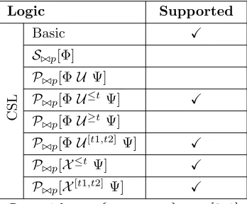
CTMCs). In PRISM it is possible to either determine if a probability satisfies a given bound or obtain the actual value. There is also support for the specification and analysis of properties based on costs and rewards, but the implementation of this feature is only partially completed (in version 2.1) and is still ongoing. The subset of PCTL and CSL formulas supported by PRISM is displayed in Table 3.1.
Table 3.1: PRISM supported logic subset
Logic Supported
P
C
T
L
Basic X
L./p[Φ]
P./p[ΦU Ψ] X
P./p[ΦU≤k Ψ] X
P./p[ΦU[k1,k2] Ψ]
C
S
L
Basic X
S./p[Φ] X
P./p[ΦU Ψ] X
P./p[ΦU≤tΨ] X
P./p[ΦU≥tΨ] X
P./p[ΦU[t1,t2] Ψ] X
P./p[X≤t Ψ]
P./p[X[t1,t2] Ψ]
P./p with ./∈ {<, >,≤,≥}, p∈[0,1]
Algorithms and data structures. PRISM offers a choice between several different algorithms
Chapter 3. Probabilistic model checker tools 31
PRISM are listed below:
• Gauss-Seidel (also backwards)
• Jacobi
• JOR (also backwards)
• Power
• SOR
The iterative methods are used for solving a system of linear equations, needed for model checking the steady-stateS and unbounded untilU operators. For the time-bounded untilU[t1,t2] operator
PRISM uses uniformization [45] and the techniques of Fox and Glynn [28].
PRISM offers the user a choice between any of the following three data structures for model checking:
1. MTBDD (Multi-Terminal Binary Decision Diagram) for model construction and BDD for reachability, more information on MTBBD/BDD’s can be found in [30,24].
2. Sparse matrix [65, 64].
3. Hybrid, a combination of MTBDD and sparse matrix.
All engines perform the same calculations; therefore the choice between “MTBDD”, “Sparse” or “Hybrid” will not affect the results of the model checking. However, according to [52], the time and space performance may differ considerably. Typically the sparse engine is quicker than its MTBDD counterpart, but requires more memory. The hybrid engine aims to provide a com-promise, providing faster computation than pure MTBDDs but using less memory than sparse matrices. By default, PRISM uses the hybrid engine.
3.2
ETMCC
E`M C2 (written ETMCC) is developed by the Stochastic Modelling and Verification group at the University of Erlangen-N¨urnberg, Germany, and the Formal Methods & Tools group at the University of Twente, the Netherlands. It is a prototype implementation of a model checker for continuous-time Markov chains. The tool is free for non-profit organizations. The user has to fill in a license agreement form before downloading and using the tool. This thesis discusses version 1.4.2, which is available at: http://www7.informatik.uni-erlangen.de/etmcc/
Implementation details. The tool is developed in Java, it requires Java version 1.2 or above
and operates on Linux, Windows and Solaris systems. ETMCC has no command line interface, all interaction must be performed using a Graphical User Interface (GUI). The GUI offers an editor for constructing properties and is used for loading all necessary input files and displaying the verification results. For our measurements, we added ad-hoc command line support to ETMCC.
Model and specification language. ETMCC supports CTMC models only1. It accepts model
descriptions in the tra-format as generated by the stochastic process algebra tool TIPPtool [35] and Petri net tool DaNAMiCS [18]. An example of thetra-format is shown in Figure3.1.
send 1 2 1.7 M receive 1 3 1 M acknowledge 3 11 1 M ...
Figure 3.1: tra-format example
1There is a trick to let ETMCC handle DTMCs, namely: let all rates be between 0 and 1 and the rates sum up
32 Chapter 3. Probabilistic model checker tools
Each line specifies one transition consisting of an action name, the source state, the target state, the transition rate and the type, which is set to M (Markovian). Note that the tra-format
also supports transition types P (probabilistic) and I (immediate), but these are not supported by ETMCC. ETMCC also accepts model description in a format called CSLstandard, which is a derivative of the tra-format, where actions and the type of transition are omitted. The state labelling with atomic propositions must be provided in a.lab file.
Properties. ETMCC supports two types of logics, namely CSL and action-based CSL (aCSL).
The subset of CSL formulas supported by ETMCC is displayed in Table 3.2. Similar to CSL, aCSL provides a means to reason about CTMCs, but opposed to CSL, it is not state-oriented. Its basic constructors are sets of actions, instead of atomic state propositions, for details see [37].
Table 3.2: ETMCC supported logic subset
Logic Supported
C
S
L
Basic X
S./p[Φ] X
P./p[ΦU Ψ] X
P./p[ΦU≤tΨ] X
P./p[ΦU≥tΨ]
P./p[ΦU[t1,t2] Ψ]
P./p[X≤tΨ]
P./p[X[t1,t2] Ψ]
P./p with ./∈ {<, >,≤,≥},p∈[0,1]
Algorithms and data structures. The model checking algorithms used by ETMMC are
de-scribed in [36, 38]. The tool offers a choice between Gauss-Seidel and Jacobi as the iterative methods used in solving steady-state and unbounded until properties. The methods for bounded until are either transient analysis (recommended) or Volterra integrals for [0;t] (less accurate, slow). ETMCC uses an explicit (i. e. not symbolic) data structure, namely a sparse matrix.
3.3
MRMC
MRMC is a model checker for discrete-time and continuous-time Markov reward models. It is distributed under the GNU General Public License (GPL). The MRMC tool is developed by the Software Modelling and Verification (MOVES) group at the RWTH Aachen University (Germany) and Formal Methods & Tools group at the University of Twente (the Netherlands). The version used is 1.1.1b. It is available at: http://www.cs.utwente.nl/~zapreevis/mrmc/
Implementation details. The developers of MRMC have used ETMCC as inspiration to build
Chapter 3. Probabilistic model checker tools 33
Model and specification language. MRMC supports four types of input models:
• DTMC
• DMRM2
• CTMC
• CMRM3
The input models are described in the same format as for ETMMC (see Section 3.2), except for the syntax related to aCSL which is not supported by MRMC. The probability (for DTMC) or rate matrix (for CTMC) is defined by a .tra file and the state labelling by a.lab file. These files contain straightforward text-based descriptions of the models. When dealing with specification and analysis of properties based on rewards, the state reward structure can be specified in a.rew
file and the impulse reward structure in a.rewi file.
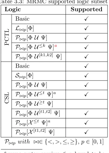
Properties. Properties can be specified using one of the following logics:
• PCTL
• PRCTL4
• CSL
• CSRL5
The subset of PCTL and CSL formulas supported by MRMC is displayed in Table3.3.
Table 3.3: MRMC supported logic subset
Logic Supported
P
C
T
L
Basic X
L./p[Φ] X
P./p[ΦU Ψ] X
P./p[ΦU≤k Ψ]a X
P./p[ΦU[k1,k2] Ψ] X
C
S
L
Basic X
S./p[Φ] X
P./p[ΦU Ψ] X
P./p[ΦU≤tΨ]a X
P./p[ΦU≥tΨ]
P./p[ΦU[t1,t2] Ψ] X
P./p[X≤tΨ]a X
P./p[X[t1,t2] Ψ] X
P./p with ./∈ {<, >,≤,≥},p∈[0,1]
a mrmc syntax requires ≤ x bound to be
specified as [0,x]
34 Chapter 3. Probabilistic model checker tools
Algorithms and data structures. For checking PCTL, MRMC uses the algorithms described
in [33], for PRCTL see [8] and for CSL see [11]. MRMC supports two algorithms for time-and reward-bounded until-formulas (CSRL). One is based on discretization [77], the other on uniformization and path truncation [67]. This includes state and impulse rewards. In combination with uniformization it used the techniques of Fox and Glynn [28]. The supported iterative methods are listed below:
• Jacobi
• Gauss-Seidel
The state-space is represented using sparse matrix with the compressed row, compressed column technique [68] (also called Harwell-Boeing sparse matrix format).
3.4
YMER
YMER(3.0) is a tool for verifying transient properties of stochastic systems. It supports Continuous-Time Markov Chains (CTMCs) and Generalized Semi-Markov Processes (GSMPs)6. YMER
im-plements statistical model checking techniques, based on discrete event simulation and acceptance sampling, for CSL model checking [83]. YMER also supports numerical techniques for CTMCs model checking. The tool is developed by H˚akan Younes at Carnegie Mellon University (Pitts-burgh). The current version is 3.0 (released February 1, 2005), which is distributed under the GNU General Public Licence (GPL). The tool is available at: http://www.cs.cmu.edu/~lorens
Implementation details. YMER is a command-line-based tool. It uses a random number
generator implemented in C, whereas other parts of the tool are written in C++. YMER uses the CUDD7package for symbolic data structures, this package is not included in the distribution and
should be installed separately. The numerical engine for model checking CTMCs is adopted from the hybrid model checker engine of the PRISM tool. The tool operates on the Linux platform, support for other platforms is not specified.
Model and specification language. YMER supports two types of input models:
• CTMC
• GSMP[80]
The language used for model specification is a subset of the PRISM language8. Because the
language is a subset, it means not all operations on for instance rate values are supported9.
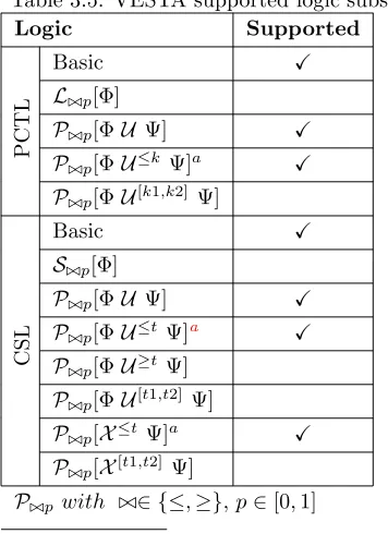
Properties. Properties can be specified using CSL. The subset of CSL formulas supported by
YMER is displayed in Table3.4.
Algorithms and data structures. For CSL model checking YMER implements the statistical
model checking techniques proposed by Younes and Simmons in [85]. YMER uses discrete event simulation [71] to generate sample execution paths and verifies a given CSL path formula over each sample path. The tool offers a choice between either taking a fixed number of samples or sequential acceptance sampling. There is also support for distributed acceptance sampling, meaning multiple machines can be used to generate samples independently. It uses a master/slave architecture to collect and process samples. The interested reader is referred to [83] for more details on this architecture. Understandably, the data structures for state-space representation
6Details on GSMPs can be found in [80].
7The CUDD package can be obtained fromhttp://vlsi.colorado.edu/~fabio/CUDD. 8The BNF grammar for YMER is listed in [82].
9In YMER it is not possible to add or subtract rate values in the model description, only multiplication and
Chapter 3. Probab