Computational and Statistical Aspects of
High-Dimensional Structured Estimation
A DISSERTATION
SUBMITTED TO THE FACULTY OF THE GRADUATE SCHOOL OF THE UNIVERSITY OF MINNESOTA
BY
Sheng Chen
IN PARTIAL FULFILLMENT OF THE REQUIREMENTS FOR THE DEGREE OF
DOCTOR OF PHILOSOPHY
Prof. Arindam Banerjee
c
Sheng Chen 2018
Acknowledgements
There are many people that have earned my gratitude for their contribution to my six-year PhD life.
First I would like to express my sincerest gratitude and appreciation to my advisor Prof. Arindam Banerjee, for his guidance, support and encouragement. He is so knowl-edgeable that every discussion with him was thought-provoking. He is also passionate about delving into technical details, which has inspired several threads of my research. Besides I have also benefited from his extraordinary skills on writing, presentation and communication. Overall I was extremely fortunate to work with Prof. Banerjee during the past few years.
Second, I am deeply indebted to Prof. Rui Kuang, who has guided me through the initial years in graduate study. His tremendous patience and thoughtful advice helped me start the PhD career in a very positive way. Without his support, there would be more obstacles and difficulties in pursuing my PhD degree. I am also grateful to Prof. Daniel Boley, Prof. George Karypis, and Prof. Jarvis Haupt for serving as my dissertation committee and for their helpful suggestions and feedbacks.
Third, I would like to extend my great thanks to my supervisors and colleagues while interning at Yahoo! Research in 2016, including Troy Chevaliar, Nikolay Laptev, Tina Liu, Yashar Mehdad, Aasish Pappu, Rao Shen, Akshay Soni, and Kapil Thadani. They have opened a door for me so that I could learn the cutting-edge technologies used in
Last but not the least, I would also like to show my gratitude to my lab mates and fellow graduate students: Soumyadeep Chatterjee, Konstantina Christakopoulou, Chintan Dalal, Miao Fan, Farideh Fazayeli, Robert Giaquinto, Hardik Goel, Andre Goncalves, Qilong Gu, Sijie He, Nicholas Johnson, Xinyan Li, Xiaoli Liu, Igor Melnyk, Dave Roe, Vidyashankar Sivakumar, Amir Taheri, Shaozhe Tao, Huahua Wang, Huanan Zhang, Wei Zhang and Yingxue Zhou. It has always been enjoyable and fruitful to discuss and work with them.
The research in this thesis was supported in part by NSF grants 1563950, 1447566, 1447574, 1422557, CCF-1451986, CNS- 1314560, 0953274, IIS-1029711, NASA grant NNX12AQ39A, and gifts from Adobe, IBM, and Yahoo.
Dedication
To God and my family
Modern statistical learning often faces high-dimensional data, for which the number of features that should be considered is very large. In consideration of various constraints encountered in data collection, such as cost and time, however, the available samples for applications in certain domains are of small size compared with the feature sets. In this scenario, statistical estimation becomes much more challenging than in the large-sample regime. Since the information revealed by small large-samples is inadequate for finding the optimal model parameters, the estimator may end up with incorrect models that appear to fit the observed data but fail to generalize to unseen ones. Owning to the prior knowledge about the underlying parameters, additional structures can be imposed to effectively reduce the parameter space, in which it is easier to identify the true one with limited data. This simple idea has inspired the study of high-dimensional statistics since its inception.
Over the last two decades, sparsity has been one of the most popular structures to exploit when we estimate a high-dimensional parameter, which assumes that the num-ber of nonzero elements in parameter vector/matrix is much smaller than its ambient dimension. For simple scenarios such as linear models, L1-norm based convex
estima-tors like Lasso and Dantzig selector, have been widely used to find the true parameter with reasonable amount of computation and provably small error. Recent years have also seen a variety of structures proposed beyond sparsity, e.g., group sparsity and low-rankness of matrix, which are demonstrated to be useful in many applications. On the other hand, the aforementioned estimators can be extended to leverage new types of structures by finding appropriate convex surrogates like the L1 norm for sparsity.
Despite their success on individual structures, current developments towards a unified iv
understanding of various structures are still incomplete in both computational and sta-tistical aspects. Moreover, due to the nature of the model or the parameter structure, the associated estimator can be inherently non-convex, which may need additional care when we consider such unification of different structures.
In this thesis, we aim to make progress towards a unified framework for the estima-tion with general structures, by studying the high-dimensional structured linear model and other semi-parametric and non-convex extensions. In particular, we introduce the generalized Dantzig selector (GDS), which extends the original Dantzig selector for s-parse linear models. For the computational aspect, we develop an efficient optimization algorithm to compute the GDS. On statistical side, we establish the recovery guarantees of GDS using certain geometric measures. Then we demonstrate that those geometric measures can be bounded by utilizing simple information of the structures. These results on GDS have been extended to the matrix setting as well. Apart from the linear model, we also investigate one of its semi-parametric extension – the single-index model (SIM). To estimate the true parameter, we incorporate its structure into two types of simple estimators, whose estimation error can be established using similar geometric measures. Besides we also design a new semi-parametric model called sparse linear isotonic model (SLIM), for which we provide an efficient estimation algorithm along with its statistical guarantees. Lastly, we consider the non-convex estimation for structured multi-response linear models. We propose an alternating estimation procedure to estimate the param-eters. In spite of dealing with non-convexity, we show that the statistical guarantees for general structures can be also summarized by the geometric measures.
Contents
Acknowledgements i
Dedication iii
Abstract iv
List of Tables xii
List of Figures xiii
1 Introduction 1
1.1 High-Dimensional Statistics . . . 3
1.1.1 Statistical Estimation and Curse of High Dimensions . . . 3
1.1.2 Surviving High Dimension: Sparsity and Convexity . . . 5
1.2 Beyond Unstructured Sparsity . . . 7
1.3 Beyond Convexity . . . 10
1.4 Contributions and Organization . . . 13
2 Preliminaries 16 2.1 Convex Analysis . . . 16
2.1.1 Convex Set . . . 16
2.1.2 Convex Function . . . 17
2.2 Convex Optimization . . . 20
2.2.1 Gradient Descent . . . 21
2.2.2 Proximal Gradient Method and Proximal Operator . . . 22
2.2.3 Alternating Direction Method of Multipliers . . . 23
2.3 Basics of Probability Theory . . . 24
2.3.1 Gaussian Random Variable . . . 25
2.3.2 Sub-Gaussian and Sub-Exponential Random Variable . . . 26
2.4 Gaussian Width and Generic Chaining . . . 29
2.4.1 Gaussian Width . . . 29
2.4.2 Generic Chaining . . . 31
3 Generalized Dantzig Selector 36 3.1 Introduction . . . 36
3.2 Optimization Algorithm . . . 38
3.2.1 Inexact ADMM for GDS . . . 38
3.2.2 Proximal Operator for k-Support Norm . . . 41
3.3 Statistical Analysis . . . 44
3.3.1 Deterministic Error Bound . . . 44
3.3.2 Error Bound with Random Design and Noise . . . 47
3.4 Experimental Results . . . 48
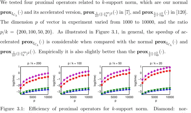
3.4.1 Efficiency of Proximal Operator . . . 49
3.4.2 Statistical Recovery . . . 49
3.A Proof of Proximal Operator fork-Support Norm . . . 51
3.A.1 Proof of Theorem 3 . . . 51
3.A.2 Proof of Theorem 4 . . . 54
3.B Proof of Statistical Guarantees . . . 57 vii
3.B.2 Proof of Theorem 6 . . . 58
4 Geometric Measures with Atomic Norms 61 4.1 Introduction . . . 61
4.2 General Upper Bounds . . . 63
4.2.1 Gaussian Width of Unit Norm Ball . . . 63
4.2.2 Gaussian Width of Error Spherical Cap . . . 65
4.2.3 Restricted Norm Compatibility . . . 67
4.3 General Lower Bounds . . . 69
4.4 Application tok-Support Norm . . . 71
4.A Supplementary Proofs . . . 74
4.A.1 Proof of Theorem 8 . . . 74
4.A.2 Proof of Lemma 9 . . . 76
4.A.3 Proof of and Theorem 11 . . . 78
5 Structure Matrix Recovery via Generalized Dantzig Selector 80 5.1 Introduction . . . 80
5.2 Deterministic Analysis . . . 83
5.2.1 Deterministic Error Bound . . . 83
5.2.2 Bounding Restricted Norm Compatibility . . . 86
5.3 Probabilistic Analysis . . . 88
5.3.1 Bounding Restricted Convexityα . . . 88
5.3.2 Bounding Regularization Parameterλn . . . 89
5.4 Examples . . . 90
5.4.1 Trace Norm . . . 90
5.4.2 Spectralk-Support Norm . . . 91
5.A Proof of Deterministic Analysis . . . 93
5.A.1 Proof of Lemma 11 . . . 93
5.A.2 Proof of Theorem 14 . . . 94
5.B Proof of Probabilistic Analysis . . . 96
5.B.1 Proof of Theorem 15 . . . 96
5.B.2 proof of Theorem 17 . . . 97
5.B.3 Proof of Theorem 16 . . . 99
6 Robust Structured Estimation for Single-Index Models 105 6.1 Introduction . . . 105 6.2 Robust Estimators . . . 109 6.2.1 Assumptions . . . 109 6.2.2 Estimators . . . 112 6.3 Statistical Analysis . . . 114 6.4 Applications . . . 116
6.4.1 1-bit Compressed Sensing . . . 116
6.4.2 A New Estimator for Monotone Transfer . . . 118
6.4.3 Other Parameter Structures . . . 121
6.5 Experimental Results . . . 122
6.A Supplementary Proofs . . . 125
6.A.1 Proof of Theorem 19 . . . 125
6.A.2 Proof ofL2-Error Bound . . . 126
6.A.3 Proof of Proposition 16 . . . 131
7 Sparse Linear Isotonic Models 133 7.1 Introduction . . . 133
7.2 Related Work . . . 136
7.4 Statistical and Algorithmic Analysis . . . 139
7.4.1 Recovery Guarantee of ˜θ . . . 140
7.4.2 Improved RE Condition . . . 145
7.4.3 Computation of F . . . 147
7.5 Experimental Results . . . 150
7.A Proof of Lemma 16 . . . 152
7.B Proof of Theorem 23 . . . 153
7.C Proof of Theorem 24 . . . 156
8 Structured Estimation for Multi-Response Linear Models 160 8.1 Introduction . . . 160
8.2 Alternating Estimation with GDS . . . 163
8.3 Statistical Analysis . . . 165
8.3.1 Estimation of Coefficient Vector . . . 168
8.3.2 Estimation of Noise Covariance . . . 173
8.3.3 Error Bound for Alternating Estimation . . . 174
8.4 Experimental Results . . . 175
8.A Proof of Statistical Guarantees for GDS . . . 178
8.A.1 Proof of Lemma 21 . . . 178
8.A.2 Proof of Lemma 22 . . . 180
8.A.3 Proof of Lemma 23 . . . 181
8.B Proof of Noise Covariance Estimation . . . 185
8.B.1 Proof of Theorem 26 . . . 185
8.B.2 Proof of Lemma 24 . . . 187
8.C Proof of AltEst Procedure . . . 188
8.C.1 Proof of Theorem 27 . . . 188 x
9 Improved Estimation for Structured Multi-Response Linear Models 190
9.1 Introduction . . . 190
9.2 Strategy to Conquer Non-Convexity . . . 193
9.3 Deterministic Analysis . . . 197 9.4 Probabilistic Analysis . . . 203 9.4.1 Preliminaries . . . 203 9.4.2 Arbitrarily-Initialized AltMin . . . 204 9.4.3 Well-Initialized AltMin . . . 208 9.5 Experimental Results . . . 210
9.A Proofs for Deterministic Analysis . . . 213
9.A.1 Proof of Lemma 25 . . . 213
9.A.2 Proof of Lemma 26 . . . 215
9.A.3 Proof of Theorem 28 . . . 217
9.B Proofs for Probabilistic Analysis . . . 218
9.B.1 Proof of Proposition 17 . . . 218 9.B.2 Proof of Lemma 27 . . . 218 9.B.3 Proof of Lemma 28 . . . 221 9.B.4 Proof of Lemma 29 . . . 222 9.B.5 Proof of Lemma 30 . . . 225 10 Conclusions 233 References 236 xi
List of Tables
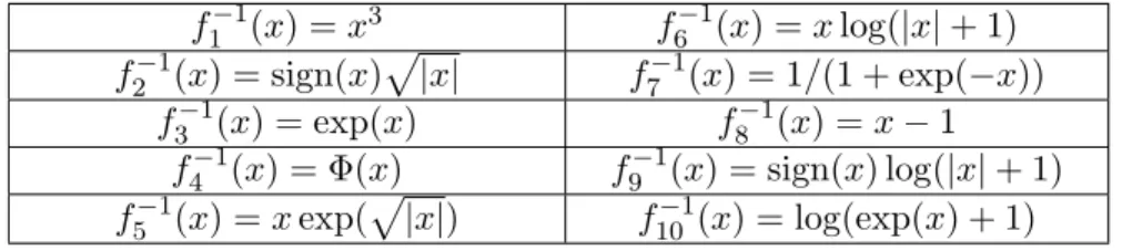
7.1 Inverse of functionfj for nonzero ˜θj . . . 151
List of Figures
1.1 Examples of structures beyond unstructured sparsity . . . 7
1.2 Convexity is more than sufficient for statistical guarantees . . . 11
3.1 Efficiency of proximal operators fork-support norm . . . 49
3.2 Statistical recovery of GDS withk-support norm . . . 50
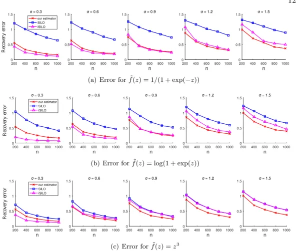
6.1 Recovery error vs. sample size . . . 123
6.2 Recovery error vs. sample size (heavy-tail) . . . 123
7.1 Error for SLIM . . . 151
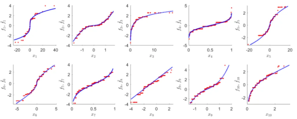
7.2 Recovery of monotone fun.ctions . . . 152
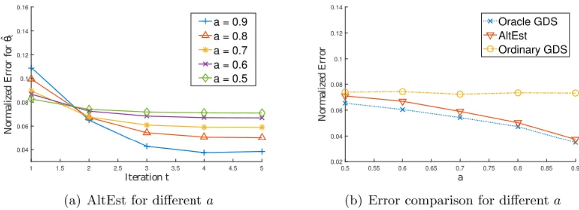
8.1 L2-error of AltEst v.s. n . . . 176 8.2 L2-error of AltEst v.s. m . . . 177 8.3 L2-error of AltEst v.s. a . . . 177 9.1 L2-error of AltMin vs. n . . . 211 9.2 L2-error of AltMin vs. a . . . 212 9.3 L2-error of AltMin vs. m . . . 212 xiii
Chapter 1
Introduction
In recent years, data-driven approaches have gained unprecedented popularity in a wide range of disciplines, such as social science, linguistics, healthcare and finance, to name a few. Numerous applications of data analysis have greatly impacted our daily life. For example, useful patterns and information are extracted from data to help people make decisions (e.g., disease diagnosis [147], portfolio selection [103] and product recom-mendation [142]). Emerging intelligent systems trained using massive data, like voice assistant and autonomous vehicles, can emancipate people from time-consuming or te-dious tasks. Moreover, the recent victory of the AlphaGo [149] against the top human go players has created a tremendous sensation, registering a peak of “Big Data”.
The success of data science critically relies on the methodology developed in machine learning and statistics. To harness the power of data, many statistical models have been proposed to describe intrinsic structures hidden in the data, and searching for the model that best explains the collected data often requires the estimation of the model parameters. Classical statistical machine learning typically deals with data arising in the low dimension, meaning that the number of features/predictors is relatively small, for which the model estimation can be performed with moderate amount of data [101]. In
2 recent years, however, high-dimensional data are frequently encountered in practice [27], where one has to consider a large set of features. Due to the expensive cost of data collection process or other constraints, it is yet difficult to gather large samples in certain scientific domain of applications, e.g., bioinformatics, climate informatics, ecology and etc. The limited sample size in comparison to the data dimension has posed significant challenges for the analysis.
In principle, the challenges brought by high-dimensional data are two-fold. In terms of methodology, data scarcity usually leads to multiple, even infinitely many models that seemingly well fit the observed data but fail to capture the true underlying pat-terns. To address the issue, we need methods that can distinguish the true model from the spurious ones. On the other hand, theoretical study for high-dimensional data also needs new treatments. In the high-dimensional regime, large-sample based asymptotic analysis [170] is not suitable for characterizing the behavior of estimators under small sample. Therefore it is necessary to derive non-asymptotic results, which provide finite-sample guarantees that hold with high probability. Aiming at the two main challenges, the research on high-dimensional statistics has made substantial progress over the last two decades. Simply put, the key philosophy behind the study of high-dimensional da-ta is the exploida-tation of prior knowledge on the model structure. Generally speaking, the source of such knowledge can be domain-specific expertise, experimental evidence or certain subjective beliefs. By enforcing the consistency between the model and the prior knowledge, we can effectively eliminate the incorrect models without using lots of data, which explains, at high level, why we can survive the high dimension. Though many previous works have demonstrated, both empirically and theoretically, that cer-tain structural priors can significantly benefit the estimation of models, attention has rarely been devoted to understanding different apriori structures in a unified framework.
To some extent, a general framework can facilitate both algorithmic design and theo-retical analysis of the estimator, as well as reveal the essence that plays a role in the estimation. Conversely, a unified understanding may inspire better ways to encode the prior knowledge. This thesis is motivated by this thread of thought.
1.1
High-Dimensional Statistics
1.1.1 Statistical Estimation and Curse of High Dimensions
Suppose that a parametric model P = {fθ | θ ∈ Θ ⊆ Rp} is proposed for a sample space Z, from which an independent and identically distributed (i.i.d.) data sample
Zn = {z1,z2, . . . ,zn} is generated with a specific parameter θ∗. The size of a data
point usually reflects theambient dimensionpof the parameter space Θ. Given the data
Zn, one of the central goals of statistical learning is to find an accurate approximation of θ∗. An estimator θˆ(Zn) is defined as a function that maps the (random) sample
Zn to an estimate in the parameter space, which is abbreviated as ˆθn or ˆθ when the
context is clear. One common way to design estimators is through the empirical risk minimization (ERM) [171] framework. In order to characterize the fitness between a single observation zi and a parameter θ, a loss function ` :Z ×Θ 7→ R is associated with the model P, and the ERM estimator tries to minimize the average of `over Zn, i.e., ˆ θERM= argmin θ∈Θ 1 n n X i=1 `(zi,θ) . (1.1)
Particularly the maximum likelihood principle is often used to specify the ERM es-timator, where the loss function ` is the negative log-likelihood of the model, i.e., `(z,θ) =−logfθ(z). In general, the estimators designed in classical statistical learning are focused on the low-dimensional setting in which n p, and the parameter space Θ is usually unrestricted and equal to Rp. The setup of the corresponding theoretical
4 studies typically assumes that n→+∞ while pis fixed. To be specific, let us consider the following simple linear model,
y=hx,θ∗i+ , (1.2)
wherex∈Rp andy∈
Rarepredictor vector andresponserespectively, and the stochas-tic noise ∼ N(0,1) is standard Gaussian. Given observed dataZn={zi = (xi, yi)}ni=1
with n > p, the maximum likelihood principle gives rise to the ordinary least squares (OLS) estimator, which estimates θ∗ by solving
ˆ θOLS= argmin θ∈Rp 1 2n n X i=1 (yi− hxi,θi)2= 1 2nky−Xθk 2 2 , (1.3)
where X = [x1,x2, . . . ,xn]T is called design matrix, and y = [y1, y2, . . . , yn]T is called
response vector. The unique solution to (1.3) can be compactly written as
ˆ
θOLS= (XTX)−1XTy , (1.4)
as long asXTXis invertible, and numerical methods can efficiently compute this solution in polynomial time [97]. Regarding the theoretical analysis, based on central limit theorem (CLT) and delta method [39], one has asymptotic normality for ˆθOLS asn→
+∞,
√
nθˆOLS−θ∗
d
−→ N 0,Σ−1 , (1.5)
in whichΣ=ExxTis thecovariance matrix forx. That is to say, for sufficiently large sample, the distribution of ˆθOLSis close toN
θ∗,Σn−1, which can be further applied to inferential tasks, such as constructinghypothesis test andconfidence set. Therefore, the study of linear models is rather complete in the low dimension for both computational and statistical aspects. The same estimation problem, however, exhibits rather different
characteristics in the high-dimensional setting. First, the OLS solution is not unique when n < p, as the columns ofXare linearly dependent. In fact, there can be infinitely many θ that fit the data perfectly (i.e., satisfy y=Xθ), from which by no means can
θ∗ be distinguished. Second, the asymptotic normality may break down even if a ˆθ can be specified, and the limiting case poorly captures the finite-sample behavior of ˆθ. In short, switching linear models to the high-dimensional regime renders the results for the low dimension meaningless. What is worse, such situation is prevalent in statistical learning.
1.1.2 Surviving High Dimension: Sparsity and Convexity
The striking differences between the high-dimensional estimation and that in low di-mension inspire the development of high-didi-mensional statistics, which concerns the esti-mation of statistical models under small sample. Since its inception [165], the core idea behind high-dimensional estimation has been centered around imposing prior structure on the true parameter θ∗, which can be fulfilled by restricting the parameter space Θ to be a strict subset of Rp. The restricted parameter space often represents a parsi-monious structure, which reflects the natural appeal to simplicity as suggested by the old principle, Occam’s razor [163]. Parsimony is not only a subjective preference in consideration of interpretability, but also supported by empirical evidence in real-world applications. One of the most well-known parsimonious structures in high-dimensional statistics is sparsity [165], which posits that θ∗ has only few non-zero elements. For instance, natural images admit sparse representations in the wavelet basis, and a text document is usually related to only a few topics out of thousands of categories. At first glance, confining the parameter space using prior knowledge seems trivial, but the subsequent estimation is in fact more challenging than it appears. Returning to the linear model, if sparsity is assumed and Θ ={θ ∈Rp | kθk
6 an s-sparse parameter space, a straightforward estimator can be obtained by extending (1.3), ˆ θ0= argmin θ∈Rp 1 2nky−Xθk 2 2 s.t. kθk0≤s . (1.6)
However, the combinatorial nature of (1.6) makes the optimization NP-hard in general, which prevents us from pursuing this direction. To bypass the computational intractabil-ity of (1.6), numbers of alternatives have been proposed to incorporate the sparsintractabil-ity. A big family of approaches are based on convexification, which basically replacesk · k0 by
its convex surrogate,L1 norm k · k1, leading to a convex program,
ˆ θcs= argmin θ∈Rp 1 2nky−Xθk 2 2 s.t. kθk1 ≤λ , (1.7)
where λ is a tuning parameter. In fact, the more widely adopted formulation is the regularized estimator, known asLasso [165],
ˆ θrg = argmin θ∈Rp 1 2nky−Xθk 2 2+λkθk1 , (1.8)
which is also a convex optimization problem. In the literature, earlier analyses have shown that under mild assumptions on the distribution of x and suitable choice of λ, the L2-error of ˆθrg satisfies
ˆ θrg−θ∗ 2 ≤O r slogp n ! , (1.9)
with high probability if the trueθ∗ iss-sparse. A similar result holds for the constrained estimator ˆθcs as well. Unlike the asymptotic result, the finite-sample bound gives an
exact dependency of error onn,pand s. More importantly, the sample size only needs to satisfy n = ω(slogp) in order to guarantee the estimation consistency, while the low dimension requires n = ω(p). The sharp contrast between the requirements on
sample size conveys a key message that additional structures of θ∗ can greatly benefit the estimation.
The topic of sparsity has also been extensively investigated in the field ofcompressed sensing (CS). The goal of compressed sensing is to estimate a sparse vector (i.e., signal) from a small number of linear measurements, which is similar to the estimation of sparse linear models. The most significant difference between the two settings is that the design matrixX in CS is often well controlled by the experimenter. The ability to manipulate the design can guarantee many nice properties, based on which several algorithms are proposed for CS, including orthogonal matching pursuit (OMP) [167] and compressive sampling matching pursuit (CoSaMP) [126], just to name a few. Though being fast in practice, these algorithms are less extensible to other settings beyond sparsity and linear measurements. Moreover, the data gleaned in statistical learning are less controllable, and the methods above can be vulnerable to the violation of the desired properties.
1.2
Beyond Unstructured Sparsity
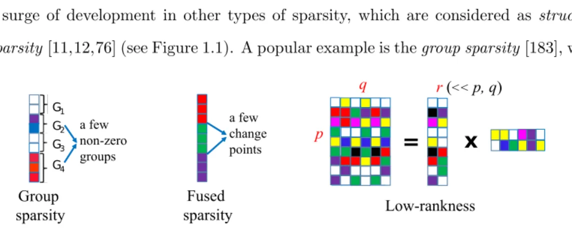
The sparsity structure introduced in Section 1.1.2 is sometimes termed as unstructured sparsity, since no additional pattern of sparsity is known. Recent years have witnessed a surge of development in other types of sparsity, which are considered as structured sparsity[11,12,76] (see Figure 1.1). A popular example is thegroup sparsity [183], where
G1 G2 G3 G4 a few non-zero groups Group sparsity a few change points Fused sparsity
=
x
p q r(<< p, q) Low-rankness8 sparsity is imposed on predefined groups of entries of θ∗ rather than the individuals. The groups themselves can be structured as well, e.g., non-overlapping, overlapping with hierarchy, and etc. Group sparsity has found numbers of specific applications in real-world problems, such as expression quantitative trait loci (eQTL) mapping in genetics [95], and sparse coding in signal processing [91]. Another widely-used structured sparsity is the fused sparsity [166], where only a small fraction of neighboring pairs in θ∗ have different values from each other. That is to say, θ∗ is piecewise constant with only few change points. Apart from the adjacency induced by the inherent one-dimensional chain structure, the elements ofθ∗can be organized as nodes of a graph, and the fused sparsity can be defined over the edges of the graph. The applications of fused sparsity include time-varying network recovery [2], DNA copy number variation (CNV) detection [164] and so on. The notion of sparsity can also be suitably generalized to matrix setting, resulting in the low-rank structure, which has been extensively exploited in the context of recommender systems [96], natural language processing [50], image analysis [33]. The low-rank structure simply assumes that the true matrix to be estimated has relatively small rank, i.e., has only few non-zero singular values. Furthermore, more complex structures can be created from simpler ones. For instance, one may assume that the true parameter simultaneously has multiple different structures [143], or it is a superposition of two or more structured components [66, 87].
Given massive interesting structures, the key to extending the aforementioned idea of convexification is to find the corresponding convex surrogate functions (usually norm-s). For the group sparsity and fused sparsity, their convex surrogates are simply given by the L2,1 group norm [183] and the total variation (TV) function [166]
respective-ly, while the low-rank structure is usually captured by the nuclear norm [141]. In the literature, there are also systematic ways to define convex surrogates, for example, via submodular function [13] andinfimal convolution [40]. Broadly speaking, the surrogate
function encodes the constrained parameter space in which θhas limited degree of free-dom, such that the preferred structure has a small function value. Computationally, using either constrained or regularized estimator with a convex loss`, we end up with a convex program that can be solved globally in polynomial time [10,24,26]. Statistically, however, the state-of-the-art understanding falls short for general structures. Earlier works [21, 174, 188] were simply focused on the unstructured sparsity, which were lat-er extended to group sparsity [75], fused sparsity [113], and etc. Those case-by-case analyses lack a general view into the key factors that determine the performance of the convex surrogates. On the contrary, a unified framework for general structures can avoid complicacies and help the analysis when we cope with new structures.
In this thesis, our first goal is committed to have a deeper understanding towards such unification. First, we concentrate on theDantzig-type estimator for linear models, which is less studied in the literature. In particular, we extend the original Dantzig se-lector [32] to the generalized Dantzig sese-lector (GDS), in order to accommodate general structures. Unlike the loss-minimization formulation in (1.7) and (1.8), the objective of Dantzig-type estimator is the convex surrogate instead of the loss, which is often non-smooth and needs extra care. Therefore, we come up with an efficient alternating direction method of multipliers (ADMM) to solve the associated optimization prob-lem. On the statistical side, we introduce the critical geometric measures – Gaussian width [63] andrestricted norm compatibility – which describe the recovery guarantees of GDS. Following that, we turn to bounding the geometric measures by utilizing simple in-formation of the structures, which largely simplifies the calculation. Moreover, we have extended those results to the matrix setting. Second, we focus on a semi-parametric extension of linear models, the single-index model (SIM), where the response is assumed to be an unknown transformation of the original linear measurement. To estimate the underlying parameter, we propose two types of simple estimators, the constrained and
10 the regularized one, based on U-statistics [98]. Under suitable conditions, the L2-error
bound of both estimators can be established using similar geometric measures. In addition to SIMs, we also propose a new semi-parametric model called sparse linear iso-tonic model (SLIM) for the high-dimensional setting, which allows nonlinear monotone transformations of the features. For SLIM, we design the computational algorithm to estimate the unknown parameter, which also leverages U-statistics. At the same time, some statistical guarantees are derived to complement the computational development of SLIM.
1.3
Beyond Convexity
As discussed in previous sections, the convexification plays a crucial role in high-dimensional estimation, which addresses the computational challenge brought by the combinatorial structure of θ∗. If the loss ` is convex, the optimization problems asso-ciated with both the constrained and the regularized estimator can be solved globally, which avoids the local optima that could be statistically erroneous. However, pursuing convexity is not always a free lunch. For certain estimation problems, such as dictio-nary learning [1] and phase retrieval [34], the natural formulation of the loss is inherently non-convex, and exploring hidden convexity (if there is any) may require skillful refor-mulations [8,37]. Furthermore the structure of the estimator ˆθobtained by using convex surrogate may slightly differ from the desired one. In some tasks, e.g., variable selection, extra effort is needed to convert ˆθ into the sought structure. Though convexity guar-antees global optimality, solving convex estimators sometimes can be computationally expensive compared with local search heuristics applied to non-convex formulations, e.g., in low-rank matrix estimation [83, 84].
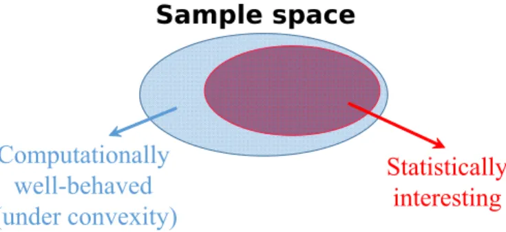
Sample space
Computationally
well-behaved
(under convexity)
Statistically
interesting
Figure 1.2: Though convexity guarantees computational optima forall data (blue) from the sample space, only asubset of them (red) are of statistical interest. The rest of data are fundamentally uninformative in the information-theoretic sense.
try non-convex estimators in high dimension, which could involve either non-convex loss-es or unconvexified functions that capture the structure of θ∗. As far as computation is concerned, non-convexity is notorious for the risk of getting trapped in local optima as well as the computational hardness, especially when discrete structures present (see (1.6) in Section 1.1.2). Despite those disadvantages, the statistical performance of non-convex estimators is often superb in practice. Such gap between the computational and the statistical aspects is rooted in the assumption on data. Without the access to unre-stricted computational resources, convexity is essential for ensuring the computational global optima for arbitraryinput data. On the contrary, statistical recovery is typically focused on generic data, since the worst-case scenario can be too pessimistic to en-counter in practice. Moreover the computational results for untypical data could fail to make any statistical sense even though they are globally optima guaranteed by convexi-ty. To see a concrete example, we revisit the linear model (1.2). Suppose that the noise is zero and the received data are of the form (xi, yi) = (0,0). In this scenario, both
L1-regularized andL1-constrained estimator always yield the estimate ˆθ=0, regardless
of the true s-sparse θ∗. Although ˆθ = 0 is the computational optimum, its statistical error can be arbitrarily large due to the pathological data. Thus convexity, to some extent, is an unnecessarily strong notion in the statistical context, which is illustrated
12 by Figure 1.2. With that being said, it is of little interest to study the computation alone without investigating the recovery guarantee, when it comes to statistical estima-tion. On the other side, the focus of statistical recovery may give us an opportunity to relax the convexity requirement and design non-convex methods tailored specifically for generic data. Guided by this thinking, the study of non-convex optimization/estimation has received considerable attention over the last few years. Several influential paper-s [20, 34, 60, 86, 159] have managed to paper-show that paper-some non-convex epaper-stimatorpaper-s can be empowered when generic data are considered. More precisely, under suitable stochastic assumptions on data, these estimators are able to recover the underlying true parameter with provably small error, which include the formulation (1.6) for sparse liner regres-sion that is nevertheless computationally infeasible in the worst case. However, like the convex setting, so far most of the related works on non-convex estimation have not yet explored the general structure of parameter, with only few exceptions [130, 154].
Motivated by both the success of non-convex optimization and the inadequate atten-tion on general structures, the second goal of this thesis is to investigate the unificaatten-tion of structured estimation under non-convexity, which parallels the goal for convex set-ting. In particular, we consider the problem of estimating multi-response linear models with general structures. Apart from the parameter vector θ∗ in vanilla linear models, here we also need to deal with the unknown noise covariance across the responses, which makes the estimation problem non-convex. We first propose an alternating estimation (AltEst) framework, a generalization of the popular alternating minimization (AltMin) procedure for non-convex optimization [82], and plug GDS in this framework to estimate both parameter vector and noise covariance. In the meanwhile, we derive the statistical guarantee for an idealized version of AltEst applied to multi-response linear models, which utilizes the same geometric measures as mentioned earlier. Second we aim at relaxing the requirement of a norm surrogate when using GDS, along with an improved
statistical analysis without assuming any idealized conditions. Specifically the GDS in the proposed AltEst framework is replaced by a constrained estimator which, from a computational perspective, is more amenable to non-norm (or non-convex) character-ization of the structure of θ∗. For the statistical analysis, by using a modified proof strategy, we are able to concentrate on the practical version of AltEst instead of the idealized one, whose theoretical guarantee is confirmed by the empirical observations.
1.4
Contributions and Organization
The main theme of this thesis is to develop both computational and statistical framework for some high-dimensional estimation problems, with an emphasis on general structures. For the computational aspect, we embrace both the idea of convexification and the non-convexity as it is, and provide algorithmic recipes for different types of estimators. On the statistical side, we focus on the L2-error analysis and establish the error bound in
terms of certain geometric measures. Moreover, we demonstrate the usefulness of these geometric measures, by deriving their further bounds for a broad class of structures. Hence our theoretical results do not leave in the bound any quantities that is hard to calculate.
The organization of this thesis is as follows.
• In Chapter 2, we provide a review for some background knowledge in probability theory, convex analysis and optimization. Also, we introduce an important notion calledGaussian width [63] along withgeneric chaining [161], an advanced tool in probability theory, which plays a key role in establishing the statistical guarantees.
• In Chapter 3, we extend the celebrated Dantzig selector for sparse linear models to accommodate general structures. As to optimization, the proposed general-ized Dantzig selector (GDS) [41] can be efficiently solved by a variant of basic
14 alternating direction method of multipliers (ADMM). In terms of statistical anal-ysis, we present a unified framework for various structures, which can succinctly characterize the error bound with certain geometric measures, such as Gaussian width.
• Chapter 4 is devoted to the study of the geometric measures introduced in Chapter 3. Those geometric measures essentially quantify the complexity of the associated structures, which need to be computed or bounded in order to determine the final error bound. For a broad class of structures that can be captured byatomic norms, we have managed to bound the geometric measures using simple information of the structure [43].
• In Chapter 5, we extend the results obtained in Chapter 3 and 4 to the matrix scenario [44], in which we have general bounds for the structures induced by the family of unitarily invariant norm.
• In Chapter 6, we study an important semi-parametric extension of linear models, thesingle-index models (SIMs), which allow the response to be anunknown trans-fer of the linear measurement. We develop two types of estimators for the recovery of model parameters [46]. With minimal assumption on noise, the statistical guar-antees are established for the proposed estimators under suitable conditions, which also allow general structures of the underlying parameter. Moreover, the proposed estimator is novelly instantiated for SIMs with monotone transfer function, and the obtained estimator can better leverage the monotonicity.
• In Chapter 7, we make an attempt to introduce some nonlinearity in the features of linear models, as opposed to the nonlinear response considered by single-index models. In particular, we propose a novel model named sparse linear isotonic model (SLIM) [47], which hybridizes the ideas in both parametric sparse linear
models and additive isotonic models (AIMs) that assume the response to be a summation of unknown monotone feature transformations. In the computational aspect, a two-step algorithm is designed for estimating the sparse parameter as well as the monotone functions. Under mild statistical assumptions, we show that the algorithm can accurately estimate the parameter.
• In Chapter 8, we focus on the non-convex estimation of structured multi-response linear models. By exploiting the noise correlations among different responses, we employ an alternating estimation (AltEst) procedure [45] to estimate the param-eters based on GDS. Under suitable sample size requirement and the resampling assumption, we show that the error of the estimates generated by an variant of AltEst, with high probability, converges linearly to certain minimum achievable level, which can be tersely expressed by the geometric measures.
• In Chapter 9, we continue to investigate the structured multi-response linear mod-els, with several extensions from Chapter 8. We allow the function encoding the structure of the parameter to be non-convex, through replacing the GDS in the AltEst framework by a constrained estimator, which results in an alternating-minimization-type algorithm. In the statistical analysis, we relax the assumption on the noise distribution. More importantly, we come up with a new analysis for the practical version of the estimator, which does not resort to any resampling assumptions. The result also reveals that random initializations of the estimation algorithm can even yield good recovery of the unknown parameter.
• Chapter 10 is dedicated to the conclusion, in which we summarize the contribu-tions of this thesis.
Chapter 2
Preliminaries
2.1
Convex Analysis
In this section, we briefly review some basics of convex analysis. Since the scope of this topic is too wide, we will just cover those used in our works for the sake of simplicity as well as keeping the self-containedness. For more complete materials, we refer interested readers to [144].
2.1.1 Convex Set
We start with the definition of convex set inRp.
Definition 1 (convex set) A set C ⊆ Rp is convex if the following holds for any
u,v∈ C,
λu+ (1−λ)v∈ C, ∀ 0≤λ≤1 . (2.1)
Examples of convex set include affine set {u |Au=b} (A∈Rq×p, b∈
Rq and q are fixed), half-space {u | hw,ui ≥β} (w∈Rp and β ∈
R are fixed), and so on. Another important instance of convex set is convex cone.
Definition 2 (cone/convex cone) A setC ⊆Rp is acone if it satisfies that
u∈ C =⇒ λu∈ C, ∀ λ >0 . (2.2)
If C is further convex, then it is aconvex cone.
Given a set A ⊆Rp, we can construct a cone by the operator cone(A) = {c·a | c ≥
0, a ∈ A}. For an arbitrary set, we can also define a special convex set called convex hull, which is its smallest convex superset.
Definition 3 (convex hull) Given any setS ∈Rp, itsconvex hull, denoted by conv(S), is the smallest convex set containing S. In particular, if S ={u1,u2, . . . ,un} is finite,
then conv(S) consists of all convex combinations of u1, . . . ,un, i.e.,
cone(S) = ( λ1u1+λ2u2+. . .+λnun n X i=1 λi= 1, λ1, λ2, . . . , λn≥0 ) (2.3) 2.1.2 Convex Function
Based on the definition of convex set, the convex function can be defined as follows.
Definition 4 (convex function) A function f : Rp 7→ R is said to be convex if its domain domf is convex and f satisfies that for anyu,v∈domf
f(λu+ (1−λ)v)≤λf(u) + (1−λ)f(v), ∀ 0≤λ≤1 . (2.4)
Specifically a convex function f is said to be proper if f(u) < +∞ for at least one u
and f(u)>−∞ for allu.
There are several useful notions related to convex functions, such as convex conjugate and gauge function (a.k.a. Minkowski functional).
18
Definition 5 (convex conjugate) For any functionf :Rp7→R, itsconvex conjugate f∗ :Rp7→R is given by
f∗(u) = sup
v∈domf
{hu,vi −f(v)} (2.5)
Note thatf∗ is always convex even iff is not. f∗ is also known asFenchel conjugate. A
special type of convex conjugate is support function, where f is theindicator function of a non-empty set S, i.e.,
IS(u) = 0, ifu∈ S +∞, otherwise . (2.6)
Definition 6 (support function) Thesupport function of a non-empty setS is given by hS(u) = sup v∈Rp {hu,vi −IS(v)}= sup v∈S hu,vi (2.7)
In some places, convex conjugate and support function are only considered for convex f andS. In this thesis, it is also sufficient to just focus on convex case.
Definition 7 (gauge function) Thegauge function(or simplygauge) of a non-empty convex set C is defined as
γC(u) = infλ≥0
u∈λC (2.8)
The gauge function is convex as well, and a useful class of gauge is norm, for which the convex set C should be bounded, centrally symmetric about the origin (i.e., u ∈ C iff.
Definition 8 (norm) Anorm k · kis a function mapping from Rp toR, which satisfies
• (positivity) kuk ≥0 ∀u∈Rp, and kuk= 0 iff. u=0
• (absolute homogeneity) kλuk=|λ| · kuk ∀u∈Rp, λ∈
R
• (subadditivity) ku+vk ≤ kuk+kvk ∀ u,v∈Rp
A dual norm k · k∗ can be defined for the original normk · k through support function,
kuk∗ = sup kvk≤1
hu,vi (2.9)
Simple examples of norm areL2 norm kuk2 = (Ppi=1u2i)1/2,L1 normkuk1 =Ppi=1|ui|,
L∞ norm kuk∞ = max1≤i≤p|ui|, and etc. The dual norm of L2 norm is itself, and L1
and L∞ norm are dual to each other. Norm plays a central role in high-dimensional
statistics, which often acts as the convex surrogate for certain structure. One nice property of dual norm is the H¨older’s inequality.
Proposition 1 (H¨older’s inequality) For any normk · k and its dual normk · k∗, it
holds that |hu,vi| ≤ kuk · kvk∗ for any u,v∈Rp.
Encompassing the norm as a special case, gauge function provides a different perspective of view into Definition 8. The closure of the convex set C that induces the normk · kis actually the (closed) unit norm ball
Ω =
u∈Rp
kuk ≤1 . (2.10)
Thus one can define the norm by specifying its unit ball, instead of giving the arithmetic expression. Such correspondence is helpful when we introduce the atomic norm [40] below.
20
Definition 9 (atomic norm) Given a compact set A that is centrally symmetric about origin and satisfies span(A) =Rp, define the atomic norm k · kA ofA by
kukA = inf ( X a∈A ca u= X a∈A caa, ca≥0 ∀a∈ A ) . (2.11)
The set Ais called atomic set, and its elementa∈ Ais called atom.
Though the expression of atomic norm seems complicated, the unit norm ball of k · kA
turns out to be simple.
Proposition 2 (unit ball of atomic norm) The unit ball of atomic norm k · kA is
the convex hull of A, i.e., ΩA = conv(A). It follow immediately from this fact that the
dual norm of k · kA is kuk∗A = sup v∈conv(A) hu,vi= sup v∈A hu,vi (2.12)
Now the definition of atomic norm may look tricky given that ΩA = conv(A), since any
norm k · kcan be made atomic norm by choosing the atomic setAto its unit ball Ω. In practice, typically we bring up this notion only when Ais finite. L1 and L∞ norm are
representative atomic norms, whose atomic sets are AL1 ={±e1,±e2, . . . ,±ep} ({ei}
denotes the standard basis of Rp) andAL∞ ={±1}p, respectively.
2.2
Convex Optimization
Convex optimization is paramount in modern machine learning and statistics, as find-ing the optimal parameters for statistical models can be often formulated as convex optimization problem. We are not intended to give a comprehensive review for every popular algorithms in the literature. Instead we will cover the basic gradient descent,
proximal gradient method, and alternating direction method of multipliers. Generally speaking, convex optimization problem (or convex program) can be cast as
min θ∈Rp
g(θ) s.t. θ ∈ C , (2.13)
where both feasible set C ⊆ Rp and objective function g :
Rp 7→ R are convex. In particular, when C =Rp, we say that the optimization problem is unconstrained. Con-vex optimization algorithms usually employ an iterative procedure to generate a se-quence of iterates, θ(0),θ(1), . . . ,θ(T) ∈ C, such that limT→∞f(θ(T)) = f( ˆθ), where
ˆ
θ = argminθ∈Cg(θ).
2.2.1 Gradient Descent
In many scenarios, we deal with unconstrained convex problems with g being smooth, which is arguably the simplest case of convex optimization. Unconstrained smooth optimization can be solved by gradient descent (GD), which iteratively performs
θ(t+1) =θ(t)−η∇g(θ(t)) (2.14)
in which η is the step size. In practice, η can vary along the iterations, e.g., can be determined by line search. The full algorithm is given in Algorithm 1. Under suitable conditions ong and step size, GD converges at rate of O(1/T), namely
g(θ(T))−g( ˆθ)≤O 1 T (2.15)
22
Algorithm 1 Gradient Descent (GD)
Input: step sizeη, number of iterationsT
Output: iterate θT 1: Initialize θ(0) 2: for t= 0 to T−1do 3: θ(t+1) =θ(t)−η∇g(θ(t)) 4: end for 5: return θ(T)
2.2.2 Proximal Gradient Method and Proximal Operator
In high-dimensional statistics, as shown in (1.7) and (1.8), we often face more complex problems, with either nontrivial constraint or non-smooth objective. The two types of estimators can be unified in a single optimization framework. Consider the following problem
min
θ∈Rp f(θ) +h(θ), (2.16)
wheref is smooth whilehis non-smooth. For constrained problem, the constraintθ∈ C
can be incorporated into h by setting h(·) = IC(·). Taking f(θ) = 21nky−Xθk22 and
h(·) =IλΩL1(·) (orh(·) =λk · k1), we recover (1.7) (or (1.8)). The problem (2.16) can be
Algorithm 2 Proximal Gradient Method (PGM)
Input: step sizeη, number of iterationsT
Output: iterate θ(T) 1: Initialize θ(0) 2: for t= 0 to T−1do 3: θ0 =θ(t)−η∇f(θ(t)) 4: θ(t+1) = argminθ∈Rp 12kθ−θ0k22+η·h(θ) 5: end for 6: return θ(T)
solved by proximal gradient method (PGM). The algorithmic description is provided in Algorithm 2. Essentially PGM executes a gradient-descent step followed by a proximal operator (or proximal mapping) (Line 4). The proximal operator is formally defined
below.
Definition 10 (proximal operator) The proximal operator proxh : Rp 7→ Rp for a closed proper convex function h is given as
proxh(u) = argmin v∈Rp 1 2ku−vk 2 2+h(v) . (2.17)
If h = IC is the indicator function for a set C, the proximal operator is also called
projection operator,
projC(u) = proxIC(u) = argmin
v∈C
1
2ku−vk
2
2 (2.18)
It can be shown that the proximal operator exists for all u ∈ Rp and is also unique.
The success of PGM heavily relies on the computation of the proximal operator being inexpensive, which is often the case for many useful h. For suitablef, the convergence rate of PGM is alsoO(1/T).
2.2.3 Alternating Direction Method of Multipliers
In machine learning and statistics, sometimes we may come across more complicated op-timization problems that involve two blocks of variables, subject to equality constraints, i.e,
min θ∈Rp
β∈Rq
f(θ) +g(β) s.t Aθ+Bβ=c , (2.19)
where f and g are both convex, but not necessarily smooth. A ∈ Rr×p, B ∈
Rr×q and c ∈ Rr are generic matrices and vector. Since the smoothness of f and g is not
guaranteed, we cannot solve (2.19) using PGM. In recent years, an popular approach to tackle such problem is thealternating direction method of multipliers (ADMM). The
24 basic idea of ADMM is to form the augmented Lagrangian,
Lρ(θ,β,µ) =f(θ) +g(β) +hµ,Aθ+Bβ−ci+
ρ
2kAθ+Bβ−ck
2
2 , (2.20)
whereµ∈Rris the dual variable, andρ >0 is a tuning parameter. Then ADMM solves the original problem by iteratively minimizingLρ w.r.t. two blocks of primal variables,
θ and β, followed by an update of dual variable µ. Algorithm 3 gives the details of ADMM. Under mild conditions on the problem (2.19), ADMM enjoys O(1/T) rate of convergence.
Algorithm 3 Alternating Direction Method of Multipliers (ADMM)
Input: tuning parameterρ, number of iterationsT
Output: iterates θ(T) and β(T)
1: Initialize β(0) and µ(0) 2: for t= 0 to T−1do 3: θ(t+1) = argminθ Lρ θ,β(t),µ(t) 4: β(t+1)= argminβ Lρ θ(t+1),β,µ(t) 5: µ(t+1)=µ(t)+ρ Aθ(t+1)+Bβ(t+1)−c 6: end for 7: return θ(T) and β(T)
2.3
Basics of Probability Theory
In this section, we will review the basics of probability theory, including the notions of sub-Gaussian and sub-exponential random variable and related concentration inequali-ties.
2.3.1 Gaussian Random Variable
Gaussian random variable (r.v. for short) is arguably the most well-known random variable in probability theory, whose density function is
f(x;µ, σ2) = √1
2πσe
−(x−µ)2
2σ2 , (2.21)
where µ and σ2 are mean and variance, respectively. The standard Gaussian r.v. has
zero-mean and unit-variance. In asymptotic setting, the limiting distributions for many statistics follow Gaussian distributions, and lots of nice properties can be shown for Gaussian random variable. We present below a few useful facts about Gaussian r.v. that are frequently utilized in this thesis work.
Proposition 3 Suppose thatx andy are two Gaussian random variables. Then xand y are independent if and only if they are uncorrelated, i.e.,
Cov(x, y) = 0 ⇐⇒ x⊥y
In general, the equivalence above does not hold for other random variables, though independence always implies uncorrelatedness. The Gaussianity can be carried to ran-dom vector too. A Gaussian ranran-dom vector (or multivariate Gaussian)x∈Rp has the
density of the form
f(x;µ,Σ) = p 1 (2π)p|Σ|exp −(x−µ) TΣ−1(x−µ) 2 , (2.22)
whereµis the mean vector andΣis the covariance matrix. Standard Gaussian random vector is referred to the one with µ=0 and Σ=I. The Gaussianity of random vector is preserved under linear transformation.
26
Proposition 4 If x ∈ Rp is a Gaussian random vector with mean µ and covariance
Σ, i.e., x∼ N(µ,Σ), then Ax∈Rq is also Gaussian for any fixed A∈Rq×p, with
E[Ax] =Aµ and Cov [Ax] =AΣAT . (2.23)
In particular, ha,xi ∼ N(aTµ,aTΣa) for anya∈Rp.
Lipschitz function of Gaussian random vector enjoys a dimensionality-independent type of concentration via isoperimetric inequalities.
Proposition 5 Let x∈Rp be a standard Gaussian random vector, and f :Rp7→R be an L-Lipschitz function. For any ≥0, we have
P(f(x)−Ef(x)> )≤exp − 2 2L2 (2.24)
2.3.2 Sub-Gaussian and Sub-Exponential Random Variable
A random variable xis sub-Gaussian if theψ2-norm defined below is finite
|||x|||ψ 2 ,sup q≥1 (E|x|q)1q √ q <+∞ (2.25)
A random vector x∈Rp is sub-Gaussian ifhx,ui is sub-Gaussian for any u∈Rp, and
|||x|||ψ
2 = supu∈Rp|||hx,ui|||ψ2. A complete introduction can be found in [172]. Next we
present some useful properties of sub-Gaussian random variables/vectors.
Proposition 6 (sub-Gaussian tail) A random variable x satisfies the following in-equality iff |||x|||ψ 2 ≤κ, P(|x|> )≤e·exp −C 2 κ2 , (2.26)
Proposition 7 (rotation invariance) Ifx1, x2, . . . , xn are independent centered
sub-Gaussian random variables, then P
ixi is also a centered sub-Gaussian random variable
with n X i=1 xi 2 ψ2 ≤C2 n X i=1 |||xi|||2ψ2 , (2.27)
where C is an absolute constant.
The rotation invariance immediately implies the well-known Hoeffding’s inequality.
Proposition 8 (Hoeffding-type inequality) Let x1, x2, . . . , xn be independent
cen-tered sub-Gaussian r.v.s, and letκ= maxi|||xi|||ψ2. Then for anya= [a1, a2, . . . , an]T ∈
Rn andt≥0, we have P n X i=1 aixi ≥ ! ≤e·exp − C 2 κ2kak2 2 , (2.28)
where C >0 is an absolute constant.
Proposition 9 If x1, x2, . . . , xp are independent centered sub-Gaussian random
vari-ables (not necessarily identical), then x= [x1, . . . , xp]T is a centered sub-Gaussian
ran-dom vector with
|||x|||ψ
2 ≤C1max≤i≤p|||xi|||ψ2 , (2.29)
where C >0 is an absolute constant.
Essentially Proposition 9 can be shown using the definition of sub-Gaussian vector and Proposition 7, which we generalize to independent sub-Gaussian vectors as follows.
Proposition 10 Ifx1,x2, . . . ,xn∈Rm are independent centered sub-Gaussian random vectors, then x = [xT1, . . . ,xTn]T ∈
28 with
|||x|||ψ
2 ≤C1max≤i≤n|||xi|||ψ2 , (2.30)
where C is an absolute constant.
Proof: Define a = [aT1,aT2, . . . ,aTn]T ∈
Smn−1, where each ai is m-dimensional. We
have |||hx,ai|||ψ 2 = n X i=1 hxi,aii ψ2 ≤ v u u tC2 n X i=1 |||hxi,aii|||2ψ2 ≤ v u u tC2 n X i=1 kaik22|||xi|||2ψ2 ≤ v u u tC2 n X i=1 kaik22·1max≤i≤n|||xi|||ψ2 =C max 1≤i≤n|||xi|||ψ2 ,
where we use Proposition 7 for the first inequality. Based on the definition of sub-Gaussian random vector, we complete the proof.
A random variable xis said to be sub-exponential if its ψ1-norm is finite, i.e.,
|||x|||ψ
1 = sup
q≥1
(E|x|q)1q
q <+∞ . (2.31)
Like sub-Gaussian random variable, some useful facts about sub-exponential variable are listed below.
Proposition 11 (sub-exponential tail) A random variable x satisfies the following inequality iff |||x|||ψ 1 ≤κ, P(|x|> )≤e·exp −C κ , (2.32)
In contrast to sub-Gaussian case, rotation invariance does not hold for sub-exponential random variable, which only yields a Bernstein-type inequality.
Proposition 12 (Bernstein-type inequality) Letx1, x2, . . . , xnbe independent
cen-tered sub-exponential random variables, and let κ = maxi|||xi|||ψ1. Then for any a =
[a1, a2, . . . , an]T and ≥0, we have P n X i=1 aixi ≥ ! ≤2 exp −C·min 2 κ2kak2 2 , κkak∞ , (2.33)
where C >0 is an absolute constant.
Sub-exponential and sub-Gaussian random variables are connected by the following proposition.
Proposition 13 A random variablexis sub-Gaussian if and only ifx2is sub-exponential.
Moreover, we have |||x|||2ψ 2 ≤ x2 ψ1 ≤2|||x||| 2 ψ2 (2.34)
2.4
Gaussian Width and Generic Chaining
In this section, we briefly introduce the concept of Gaussian width and the important probability tool called generic chaining. These topics are Interested readers are recom-mended to
2.4.1 Gaussian Width
30
Definition 11 (Gaussian width) The Gaussian width w(A) of a set A ⊆Rp is
de-fined as w(A),E sup u∈A hu,gi , (2.35)
where g∈Rp is a standard Gaussian random vector.
The Gaussian width w(A) provides a geometric characterization of the complexity of the set A. We present three perspectives of view to understand the Gaussian width. First, consider the Gaussian process {Zu}u∈A where the constituent Gaussian random
variables Zu = hu,gi are indexed by u ∈ A, and g ∼ N(0,Ip×p). Then the Gaussian
widthw(A) can be viewed as the expectation of the supremum of the Gaussian process
{Zu}. Second, hu,gi can be viewed as a Gaussian random projection of each u ∈ A
to one dimension, and the Gaussian width simply measures the expectation of largest value of such projections. Third, if A is the unit ball of a norm k · k, i.e., A = Ω, then w(A) =E[kgk∗] by definition of the dual norm. Thus, the Gaussian width is the
expected value of the dual norm of a standard Gaussian random vector. For instance, if Ais unit ball of L1 norm, then w(A) =E[kgk∞]. Below we provide some simple yet
useful properties of the Gaussian width of set A ⊆Rp:
• (monotonicity) w(A)≤w(B) for any A ⊆ B
• (positive homogeneity) w(A) =c·w(A) for anyc >0
• (convexification invariance) w(A) =w(conv(A))
• (rotation invariance) w(UA) =w(A) for any unitary matrix U∈Rp×p
• (translation invariance) w(A+b) =w(A) for any fixed b∈Rp
The following result for Gaussian width is useful when we deal with union of sets, which is extracted from Lemma 2 in [118].
Lemma 1 (Gaussian width for union of sets) LetM >4,A1,· · · ,AM ⊂Rp, and
A=∪mAm. The Gaussian width of A satisfies
w(A)≤ max
1≤m≤Mw(Am) + 2 supz∈Akzk2
p
logM (2.36)
The concept of Gaussian width can be directly extended to the matrix setting, and w(A) for setA ⊆Rd×p is given as
w(A),EG sup Z∈A hhG,Zii , (2.37)
in which hh˙,ii˙ denotes the matrix inner product, i.e., hhA,Bii = Tr(ATB) for any
A,B∈Rd×p. HereG∈Rd×p is a random matrix with i.i.d. standard Gaussian entries, i.e., Gij ∼ N(0,1). The aforementioned properties also hold for the matrix case.
2.4.2 Generic Chaining
One important tool that we use in our probabilistic argument is generic chaining [161, 162], which is powerful for bounding the suprema of stochastic processes. Suppose
{Zt}t∈T is a centered stochastic process, where eachZt is a centered random variable.
We assume the index set T is endowed with some metric (distance function)s(·,·). A key notion in generic chaining is γ2-functional γ2(T, s), which is defined for the metric
space (T, s). One can think of γ2-functional as a measure of the size of set T w.r.t.
metric s. For self-containedness, we give the expression ofγ2(T, s).
γ2(T, s) = inf {Pn} sup t∈T X n≥0 2n/2·diam (Pn(t), s) , (2.38)
where {Pn}∞n=0 = {P0,P1, . . . ,Pn, . . .} is a sequence of partitions for T, which satisfy
that|P0|= 1,|Pn| ≤22nforn≥1, and thatP
32
Q ∈ Pn+1 is a subset of some Q0 ∈ P
n. Pn(t) denotes the subset of T that containst
in the n-th partition, and diam (Pn(t), s) measures the diameter ofPn(t) w.r.t. metric
s(·,·). Note thatγ2-functional is a purely geometric concept, which involves no
probabil-ity. Given that γ2-functional is fairly involved, we are not going to discuss any insights
behind this definition, and refer interested readers to the introductory books [161, 162]. Based on its definition, we list a few straightforward properties of γ2-functional here.
γ2(T, s1)≤γ2(T, s2) ifs1(u,v)≤s2(u,v),∀ u,v∈ T (2.39)
γ2(T, βs) =β·γ2(T, s) for any β >0 . (2.40)
γ2(T1, s1) =γ2(T2, s2) if∃ a global isometry between (T1, s1) and (T2, s2) (2.41)
The following lemma concerned with the suprema of{Zt}combines Theorem 2.2.22 and
2.2.27 from [162].
Lemma 2 Given metric space(T, s), if the associated centered stochastic process{Zt}t∈T
satisfies the condition
P(|Zu−Zv| ≥) ≤ C0exp − C1 2 s2(u,v) , ∀ >0 and u,v∈ T , (2.42)
then the following inequalities hold
E sup t∈T Zt ≤C2γ2(T, s) , (2.43) P sup u,v∈T |Zu−Zv| ≥C3(γ2(T, s) +·diam (T, s)) ! ≤C4exp −2 , (2.44)
where C0, C1, C2, C3 and C4 are all absolute constants.
Lemma 3 (Theorem D in [125]) There exist absolute constants C1, C2 for which
the following holds. Let(Ω, µ)be a probability space on whichxis defined, andx1, . . . , xn
be independent copies of x. Let set Hbe a subset of the unit sphere of L2(µ), i.e.,
H ⊆SL2 = ( h : |||h|||L 2 = s Z Ω h2(x)dx= 1 ) , (2.45)
Assume that suph∈H |||h|||ψ2 ≤κ. Then, for anyβ >0 and n≥1 satisfying
C1κ·γ2(H,|||·|||ψ2)≤β
√
n , (2.46)
with probability at least 1−exp−C2β2n
κ4 , sup h∈H 1 n n X i=1 h2(Xi)−Eh2 ≤β . (2.47)
The suprema in both Lemma 2 and 3 are characterized in terms ofγ2-functional, which
is not easily computable. In order to further bound the γ2-functional, one needs the
so-called majorizing measures theorem [160].
Lemma 4 Given any Gaussian process {Yt}t∈T, define s(u,v) =
p
E|Yu−Yv|2 for
u,v∈ T. Then γ2(T, s) can be upper bounded by
γ2(T, s)≤C0E sup t∈T Yt , (2.48)
where C0 is an absolute constant.
In the analysis, we usually instantiate this lemma by constructing the simple Gaussian process {Yt = ht,gi}t∈T for any T ⊆ Rp, where g is a standard Gaussian random vector. Hence s(u,v) = p
E|Yu−Yv|2 = p
34 Lemma 4 that γ2(T,k · k2)≤C0E sup t∈T ht,gi =C0·w(T) , (2.49)
which makes the connection between γ2-functional and Gaussian width. For matrix
setting, we can also get such connection by a similar construction of the Gaussian process, γ2(A,k · kF)≤C0E sup Z∈A hhG,Zii =C0·w(A) , (2.50)
where the setA ∈Rd×p.
combining Lemma 2 and 4, we can get the following theorem, which is more amenable to some of the proofs.
Theorem 1 Let {Zt}t∈T be a stochastic process indexed by T ⊆Rp, which satisfies sup t,t0∈T |||Zt−Zt0||| ψ2 kt−t0k2 ≤K <+∞
There exist absolute constants C0 andC1 such that the following bound holds with
prob-ability at least 1−C1exp
− w2(T) diam2(T) , sup t,t0∈T |Zt−Zt0| ≤C0K·w(T) , (2.51)
where diam (T) = supt,t0∈T kt−t0k2.
In the analysis, sometimes we need to bound product processes, which can be dealt with by the following theorem. The result is essentially a simplified form of Theorem 1.13 in [124]. The original theorem is stated in terms of a variant of the γ2-functional
defined above, and contains a few more tunable variables, both of which are not central to the core idea and thus have been hidden. The bound here is expressed using Gaussian width.
Theorem 2 Let (Ω, µ) be a probability space, and Z1, Z2, . . . , Zn be an i.i.d. sample
distributed according to µ. Suppose that F = {fa}a∈A and H = {hb}b∈B are two
function classes defined on(Ω, µ), which are indexed byA ⊆Rp andB ⊆
Rq respectively. Assume that sup f∈F |||f|||ψ 2 ≤RF <+∞ , sup h∈H |||h|||ψ 2 ≤RH<+∞ , sup a,a0∈A |||fa−fa0||| ψ2 ka−a0k2 ≤KF <+∞ , sup b,b0∈B |||hb−hb0||| ψ2 kb−b0k2 ≤KH<+∞ , and denote ε= min KF·w(A) RF , KH·w(B) RH .
There exist absolute constants C0, C1 and C2 such that if n ≥ C0ε2, the following
inequality holds with probability at least 1−2 exp −C1ε2
, sup f∈F sup h∈H 1 n n X i=1 f(Zi)h(Zi)−E[f h] ≤ C2· RHKF·w(A) +RFKH·w(B) √ n (2.52)
The theorem above immediately leads to the following corollary, which is similar to Lemma 3 but more flexible in some situations.
Corollary 1 Under the setting of Theorem 2, ifF =HandA=B, then there exist ab-solute constants C0,C1 andC2 such that if n≥C0
K
F·w(A)
RF 2
, the following inequality holds with probability at least 1−2 exp
−C1 K F·w(A) RF 2 , sup f∈F 1 n n X i=1 f2(Z i)−Ef2 ≤ C2· RFKF·w(A) √ n (2.53)
Chapter 3
Generalized Dantzig Selector
3.1
Introduction
The Dantzig Selector (DS) [21, 32] provides an alternative to regularized regression approaches such as Lasso [165, 188] for sparse linear estimation. While DS does not consider a regularized maximum likelihood approach, [21] has established clear simi-larities between the estimates from DS and Lasso. While norm regularized regression approaches have been generalized to more general norms, such as decomposable norm-s [127], the literature on DS hanorm-s primarily focunorm-sed on the norm-sparnorm-se L1 norm case, with
a few notable exceptions which have considered extensions to sparse group-structured norms [112]. Here we consider linear models of the form
y=Xθ∗+ , (3.1)
where y ∈ Rn is a set of observations, X ∈
Rn×p is a design matrix, and ∈Rn is a noise vector of i.i.d. entries. For anygiven norm k · k, the parameterθ∗ is assumed to be structured so that kθ∗k is of small value. For this setting, we propose the following