Cziva, R., Anagnostopoulos, C. and Pezaros, D. P. (2018) Dynamic,
Latency-Optimal vNF Placement at the Network Edge. In: IEEE
Conference on Computer Communications (INFOCOM 2018), Honolulu,
HI, USA, 15-19 Apr 2018, pp. 693-701. ISBN 9781538641286
(doi:
10.1109/INFOCOM.2018.8486021
)
This is the author’s final accepted version.
There may be differences between this version and the published version.
You are advised to consult the publisher’s version if you wish to cite from
it.
http://eprints.gla.ac.uk/153654/
Deposited on: 09 January 2018
Enlighten – Research publications by members of the University of Glasgow
http://eprints.gla.ac.uk
Dynamic, Latency-Optimal vNF Placement
at the Network Edge
Richard Cziva, Christos Anagnostopoulos and Dimitrios P. Pezaros
School of Computing Science, University of Glasgow, Glasgow, G12 8QQ, Scotland
[email protected], [email protected], [email protected]
Abstract—Future networks are expected to support low-latency, context-aware and user-specific services in a highly flexible and efficient manner. One approach to support emerging use cases such as, e.g., virtual reality and in-network image processing is to introduce virtualized network functions (vNF)s at the edge of the network, placed in close proximity to the end users to reduce end-to-end latency, time-to-response, and unnecessary utilisation of the core network. While placement of vNFs has been studied before, it has so far mostly focused on reducing the utilisation of server resources (i.e., minimising the number of servers required in the network to run a specific set of vNFs), and not taking network conditions into consideration such as, e.g., end-to-end latency, the constantly changing network dynamics, and user mobility patterns.
In this paper, we first formulate the Edge vNF placement
problem to allocate vNFs to a distributed edge infrastructure, minimising end-to-end latency from all users to their associated vNFs. Furthermore, we present a way to dynamically re-schedule the optimal placement of vNFs based on temporal network-wide latency fluctuations using optimal stopping theory. We evaluate our dynamic scheduler over a simulated nation-wide backbone network using real-world ISP latency characteristics. We show that our proposed dynamic placement scheduler minimises vNF migrations compared to other schedulers (e.g., periodic and always-on scheduling of a new placement), and offers Quality of Service guarantees by not exceeding a maximum number of latency violations that can be tolerated by certain applications.
Keywords—Network Function Virtualization, Latency, Edge Network, Resource Orchestration, Optimal Stopping Theory
I. INTRODUCTION
The penetration of Content Delivery Networks (CDN) in recent years has demonstrated the benefits of deploying application-aware intelligence in the network. Continuing in this direction and building on Software-Defined Networking (SDN), future telecommunication networks are now expected to support low-latency, context-aware and uspecific ser-vices (also called ”value-added” serser-vices) carrying large vol-umes of traffic while being managed in a highly flexible and efficient manner [1]. Example applications include high-definition low-latency video encoders and content caches, web and P2P index engines, personalised firewalls and security functions, and tactile Internet and virtual or augmented reality applications that demand fast and low-latency in-network data processing.
One approach to support these emerging use cases of the future Internet is to introduce and manage virtualized network services (also called virtual Network Functions or vNFs) not only at the provider’s internal Network Function Virtualization (NFV) infrastructure, but also at the distributed
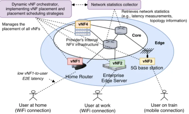
Fig. 1: A high-level architecture of the system; the dynamic orchestrator manages the placement of all vNFs and continu-ously monitors the dynamics of network properties.
Multi-Access Edge Computing (MEC) infrastructure of the network [2] [3]. Edge computing devices can include home routers managed by the ISP of the user, IoT or enterprise gateways that connect many users to the Internet, as well as next generation base stations equipped with storage and computing capabilities, as shown in Figure 1. In order to run services at the network edge, one can use virtualization technologies such as Virtual Machines or more preferably lightweight Linux containers (e.g., LXC or Docker) that allow vNFs to be placed even on low-cost devices (e.g., home routers), as presented in [4]. However, while placing vNFs near end-users radically reduces vNF-to-user end-to-end (E2E) latency (the latency experienced between an end-user and the associated vNF), time-to-response, and unnecessary utilisation of the core network, the location of edge vNFs has to be carefully managed to accommodate movements of end-users (that are expected to happen constantly due to the small cell sizes of next generation mobile architecture (5G)) and also to keep up with varying traffic dynamics that cause highly variable latency across network links [5] [6].
Orchestration and placement of vNFs has been one of the main NFV research challenges due to the complexity of service chains and the dynamics of the emerging traffic patterns. While many research projects have proposed solutions for static vNF placement (e.g., [7], [8]), to the best of our knowledge, placement of vNFs in a distributed edge NFV infrastructure has not been studied before. Furthermore, most NFV resource orchestration schemes calculate placement only for a specific service chain using a static network condition (topology and
traffic) and do not re-compute placement to migrate vNFs when these temporal network properties change. The lack of dynamic orchestration and re-calculation of vNF placement often results in “latency violations” for users, where vNF-to-user E2E latency exceeds a desired value (e.g., latency violation is when a video cache vNF has an upper bound of 100 ms for vNF-to-user E2E latency, but due to network congestion the actual vNF-to-user E2E latency increases to 130 ms for a period of time). On the other hand, the number of vNF migrations triggered by re-optimising the placement of vNFs has to be minimised since vNF migrations cause temporal service interruption and high network overhead while transferring their state across physical hosting devices [9].
Contribution & Research Outcome: In this paper, we advocate thatEdge vNFsneed to be dynamically placed in syn-ergy with changing network dynamics (e.g., latency fluctuating on links), user demands (e.g., certain vNFs are used in certain times of the day) and mobility (e.g., users move continuously with the mobile devices) to support low vNF-to-user E2E latency. Our main contributions are: (i) we formulate and solve “Edge vNF placement”, a realistic vNF placement problem; (ii) we provide a time-optimised scheduler that strives to achieve latency-optimal allocation of vNFs in next-generation Edge networks using the fundamentals of optimal stopping theory [10]; and (iii) we provide the mathematical analyses and theorems for the considered dynamic re-calculation of the optimal vNF placement. We show that by re-calculating the optimal placement and migrating vNFs at a carefully selected time, unnecessary vNF migrations can be prevented (saving resources for the operators), while the number of latency violations in the network is always bound. We present experimental results using a simulated nation-wide network based on real-world latency characteristics and vNF latency requirements.
The remainder of this paper is structured as follows. We formulate the basic placement model in Section II and intro-duce the dynamic scheduling in Section III. In Section IV, we evaluate our proposed placement and our dynamic scheduler using various experiments comparing number of migrations performed and latency violations encountered by diverse place-ment scheduling schemes. Section V discusses related work, and Section VI concludes the paper.
II. OPTIMALEDGE VNFPLACEMENT
In this section, we introduce and formalise the Edge vNF placement problem as an Integer Linear Program (ILP) to calculate the latency-optimal allocation of vNFs in next-generation edge networks.
A. Rationale
With recent advances of virtualization and NFV, vNFs can be hosted on any physical server, for instance an edge device close to the user or in a distant cloud [11] [3] [12]. In order to provide the best possible vNF-to-user E2E latency, the operators are aiming to place vNFs in close proximity to their users, by first utilising edge devices that are close to the user and falling back to hosting vNFs in the provider’s internal cloud when edge devices are out of capacity. We
Network parameters Description
G= (H,E,U) Graph of the physical network.
H={h1, h2, hj, . . . , hH} Compute hosts (e.g., edge devices) within the
network.
E={e1, e2, em, . . . , eE} All physical links in the network.
U={u1, u2, uo, . . . , uU} All users associated with network functions.
P={p1, p2, pk, . . . , pP} All paths in the network.
Wj Hardware capacity{cpu, memory, io}of the
hostshj∈H.
Cm Capacity of the linkem∈E.
Am Latency on the linkem∈E.
Zk Last host in pathpk∈P.
vNF parameters Description
N={n11, n22, noi, . . . , nUN} Network functions to allocate, where the vNF
noi∈Nis associated to useruo∈U.
Ri vNF’s host requirements {cpu, memory, io}
of vNFni∈N.
θi The maximum latency vNFni ∈ N tolerates
from its user.
Derived parameters Description
bijk Bandwidth required between the user and the vNF
niin case it is hosted athj using the pathpk.
Derived from the physical topology and the vNF requests.
lijk Latency between the user of the vNFniin case
it is hosted athjand uses the pathpk. Derived
from the physical topology and the vNF requests.
Variables Description
Xijk Binary decision variable denoting ifniis hosted
athj using the pathpkor not.
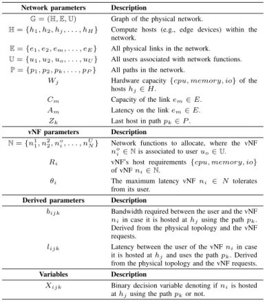
TABLE I: Table of parameters for our System model.
also accommodate different bandwidth requirements of various types of vNFs.
B. System Model
Table I shows all the parameters used for the formulation. We represent the physical network as an undirected graph G= (H,E,U), whereH,EandUdenote the set of hosts, the links between them, and the users in the topology, respectively. We assume that vNFs can be placed to any host in this graph, meaning that all physical hosts have cpu, memory, io
capabilities to host vNFs. Also, we assume that all links have a physical limit on their bandwidth (e.g., 1 Gbit/s or 100 Mbit/s) that is taken into account for the placement.
As there are different types of vNFs (e.g., lightweight firewalls or resource-intensive Deep Packet Inspection mod-ules), we introduce cpu, memory, io requirements for each
ni. On top of the compute requirements, all vNFs have delay requirements according to the service provider’s Service Level Agreements (SLA) that are denoted withθi. Similarly, all vNFs specify bandwidth reservations required along the path from their user (since some vNFs are used heavily by the users, some are not). These bandwidth requirements are materialised using the derived parameter bijk that denotes the bandwidth required along the pathpk in case vNFnoi (vNF associated to
useruo) is hosted at hj. Another important derived parameter of the model,lijk, denotes the latency from a user to a vNF in caseno
i vNF is hosted at a certain host (hj) while its traffic is
routed using a certain path pk.lijk is calculated by summing all Am individual latency values of each link along the path pk from useruo (user of vNF noi) to the vNF hosted at host
hj. Finally, let Xijk be our main binary decision variable for the model, that is:
Xijk =
1 if we allocate no
i tohj using path pk
0 otherwise (1)
C. Problem Formulation for Optimal Placement
The Edge vNF placement problemis defined as follows:
Problem 1. Given the set of usersU, the set of vNF hostsH,
the set of individual vNFsN, and a latency matrixl, we need
to find an appropriate allocation of all vNFs that minimises the total expected end-to-end latency from all users to their respective vNFs: min. X pk∈P X no i∈N X hj∈H Xijklijk (2)
Eq. 2 looks for the values of Xijk, while it is subject to the following constraints:
X no i∈N X pk∈P XijkRi< Wj,∀hj ∈H (3) X hj∈H X pk∈P Xijklijk< θi,∀no i ∈N (4) X hj∈H Xijk= 1,∀no i ∈N,∀pk∈P (5) X hj∈H Xijkbijk< Cm,∀em∈pk,∀pk ∈P (6) Xijk= 0, noi 6=Zk,∀nio∈N,∀pk ∈P,∀hi∈H (7) Constraint (3) ensures that the hardware limitations of hosts are adhered to (since CPU, memory, and IO resources are finite, we can only host a certain number of vNFs at particular hosts). Constraint (4) ensures that the maximum vNF-to-user E2E latency tolerance (θi) is never exceeded at placement. Constraint (5) states that each vNF must be allocated to exactly one of the hosts (for instance to a nearby edge device or the Cloud), while constraint (6) takes bandwidth requirements of vNFs (bijk) and link capacities (linkcap(m)) along a path, and ensures that none of the physical links along the path get overloaded. Finally, constraint (7) ensures that the selected user-to-vNF path is valid, meaning that it ends with the host of the vNF.
III. DYNAMICPLACEMENTSCHEDULING
In this Section, we present a way to schedule the re-computation of the placement presented in Section II to fit a real-world scenario, where the E2E user-to-vNF latency changes over time due to events such as congestion on any of the links in the path or user mobility resulting in a longer path between the user and the vNF [13].
A. Rationale
After a vNF placement is retrieved by implementing and running the ILP model presented in (Section II), the binary decision variablesXijk=xijk are instantiated to the values 0 or 1, such that the objective latency function F({xijk, lijk})
is minimised w.r.t. latency values lijk. Let us denote this instantiation I0. Now, we have to consider a dynamic
envi-ronment where the latency matrixlijk between vNFilocated
at host j using pathkvaries with time due to, e.g., temporal load variation at the vNF hosting platform, the position (i.e., physical distance) of the user from the vNF, temporal network utilisation, etc. This implies that lt
ijk varies with time t, and
hence the overall latency Ft = Pi,j,kxijklijkt varies with
time given an initial vNF placementI0. This time dependency
evidently results to changes in the objective functionF which indicates that, at some time instance t, the placement I0
may not minimize Ft. In this case, one should re-evaluate the minimisation problem (Section II) with up-to-date latency values, hence obtaining anewvNF placementItat every time
instance.
Based on a new vNF placement, vNFs might be needed to migrate from one host to another in order for the new placement It to minimise the objective function (overall
minimum latency) Ft. This migration cost due to different placement configurations is non-negligible. Specifically, given placements It and Iτ at time instances t and τ withτ > t, respectively, that both minimise the expected latenciesFtand
Fτ, respectively, the migration costMt→τ is defined as:
Mt→τ =
X
ijk
I(xtijk, xτijk), (8) with I(x, x0) = 0 if x=x0, and 1 otherwise. We encounter the problem to determine when a new optimal vNF place-ment needs to be evaluated to avoid possibly redundant re-computation and additional cost for vNF migration from one host to another. The trade-off here is that, at time instanceτ > t, we cantoleratesomedeviationfrom the optimal (minimum) latency computed at time instance t to void a new optimal placement at τ along with a possible migration cost Mt→τ
with expected migration cost E[Mt→τ] =nhP(xtijk =x τ ijk),
wherenis the number of users andhis the number of hosts. To materialise this tolerance, we assume that a vNFican tolerate some latency increase, up to itsθi. As a real-world example, a strictly real-time packet processing vNF can have a maximum of 10 ms latency tolerance [14]. That is, we define as vNF
latency tolerance violation at timetas the indicator:
Ltijk=
1 if lt ijk > θi
0 otherwise (9)
Since each vNF is only using one path and is allocated to one server, a single vNF’s tolerance can be defined as:
Lit=X
j X
k
Ltijk, (10)
while, at timet, the violation tolerance for all vNFs is then:
Lt=X
i
We are monitoring the evolution of the overall violation toler-anceLtwith time in order to determine when to re-evaluate the optimisation placement problem in light of minimising the cost of migration. In the remainder, we employ Optimal Stopping Theory principles to formalise this dynamic decision making problem.
B. Problem Formulation for Dynamic Placement Scheduling
Let us accumulate the user’s violations in terms of latency tolerance from time instance t = 0, where we obtained the optimal placements of all the vNF by minimisingF, up to the current time instancet, i.e., we obtain the following cumulative sum of overall violations up to t:
Yt=
t X
k=0
Lk. (12)
Given the initial optimal placement I0, latency tolerance θi
per vNF i, and expected migration cost E[M0] independent
of time, we require that the maximum latency toleration of the system users should not exceed a tolerance threshold Θ>0. That is, at any time instance t, if Yt ≤ Θ then we do not enforce a re-evaluation of the vNFs placement, hence avoid incurring any possible vNF migration cost M0→t. If Yt >
Θ, then we should re-compute a new optimal placement and incur an expected migration cost E[M0→t]. We allow Θ to
be carefully set and adjusted by operators to reflect a specific QoS level and control the rate of latency violations allowed. We can also extend the model to implement various QoS levels by setting up different values of Θ for diverse sets of users (e.g., subscribers paying for a premium vNF service have a lowerΘthan other flat-charged customers).
The challenge is to find the (optimal stopping) time in-stance t∗ for deriving an optimal placement for the vNFs, such that Yt be as close to the system’s maximum tolerance
Θas possible. This Θcan then reflect the Quality of Service offerings of the network provider. IfYtexceeds this threshold, then we incur a given expected vNF migration cost E[M0].
Specifically, our goal is to maximise the cumulative sum of tolerances up to time twithout exceedingΘ. To represent this condition of minimising the distance of the cumulative sum of violations from the maximum tolerance Θ, we define the following reward function:
f(Yt) =
Yt if Yt≤Θ, λE[M0] ifYt>Θ,
(13) where factorλ∈[0,1]weighs the importance of the migration cost to the reward function. Formally, the time-optimised problem is defined as finding the optimal stopping time t∗
that maximises the expected reward in (13):
Problem 2. Find the optimal stopping time t∗ where the supremum in (14) is attained:
sup
t≥0E
[f(Yt)]. (14)
The solution of Problem 2 is classified as an optimal stopping problem where we seek a criterion (a.k.a. optimal stopping rule) when to stop monitoring the evolution of the cumulative sum of overall violations in (12), and start off a
new re-evaluation of the optimisation for deriving optimal vNF placements. Obviously, we can re-evaluate the vNF placement optimisation algorithm at every time instance, but this comes at the expense of frequent vNF migrations. On the other hand, we could delay the re-evaluation of the optimal placement at the expense of a higher deviation from the initial optimal solution, since we are dealing with a dynamic environment w.r.t. latency. The idea is to tolerate as much latency violations as possible w.r.t. Θbut not to exceed this. The optimal stopping rule we are trying to find will provide an optimal dynamic decision-making rule for maximising the expected reward (sinceYtis a
random variable) from any other decision-making rule. Before proceeding with proving the uniqueness and the optimality of the proposed optimal stopping rule, we outline some essential preliminaries of the theory of optimal stopping below.
C. Solution Fundamentals
The theory of optimal stopping [15], [10] is concerned with the problem of choosing a time instance to take a certain action in order to maximise an expected payoff. A stopping rule problem is associated with:
• a sequence of random variables Y1, Y2, . . ., whose joint
distribution is assumed to be known;
• and a sequence of reward functions (ft(y1, . . . , yt))1≤t
which depend only on the observed values y1, . . . , yt of
the corresponding random variables.
An optimal stopping rule problem is described as follows: We are observing the sequence of the random variable(Yt)1≤t
and, at each time instancet, we choose either tostopobserving and apply our decision (which, in this case, is the re-evaluation of our optimal vNF placement and possible vNF migration) or continue (with the existing vNF placement without re-evaluating its optimality). If we stop observing at time instance
t, we induce a reward ft ≡ f(yt). We desire to choose
a stopping rule or stopping time to maximise our expected reward.
Definition 1. An optimal stopping rule problem is to find the optimal stopping time t∗ that maximises the expected reward:
E[ft∗] = sup0≤t≤T E[ft]. Note,T might be∞.
The information available up to time t, is a sequenceFt
of values of the random variablesY1, . . . , Yt(a.k.a. filtration). Definition 2. The 1-stage look-ahead (1-sla) stopping rule refers to the stopping criterion
t∗= inf{t≥0 :ft≥E[ft+1|Ft]} (15)
In other words, t∗ calls for stopping at the first time instance t for which the reward ft for stopping at t is (at
most) as high as the expected reward of continuing to the next time instancet+ 1 and then stopping.
Definition 3. LetAtdenote the event{ft≥E[ft+1|Ft]}). The
stopping rule problem is monotone if A0 ⊂ A1 ⊂A2 ⊂. . .
almost surely (a.s.)
A monotone stopping rule problem can then be expressed as follows: At is the set on which the 1-sla rule calls for
that, if the 1-sla rule calls for stopping at timet, then it will also call for stopping at time t+ 1 irrespective of the value of Yt+1. Similarly, At ⊂At+1 ⊂At+2 ⊂. . . means that, if
the 1-sla rule calls for stopping at time t, then it will call for stopping at all future times irrespective of the values of future observations.
Theorem 1. The 1-sla rule is optimal for monotone stopping rule problems.
We refer the interested reader to [15] for proof.
In the remainder, we propose a 1-sla stopping rule which, based on Theorem 1, is optimal for our Problem 2.
D. Optimally-Scheduled vNF Placement
At the optimal stopping timet∗, we re-evaluate the optimal placement of the vNFs, i.e., deriving the newoptimal place-ment It∗ and incur a migration expected cost E[M0] given that λ >0.
Theorem 2. Given an initial optimal vNF placement I0 at
time t = 0, we re-evaluate the optimal placement It at time instancet such that:
inf τ≤0{τ: Θ−Yτ X `=0 `P(L=`)≤(Yτ−λE[M0])(1−FL(Θ−Yτ))} (16)
whereFL(`) =P`l=0P(L=l)and P(L=`)is the cumula-tive distribution and mass function of Lin (11), respectively.
Proof:The target is to find an optimal 1-sla stopping rule, that is to find the criterion in (15) to stop observing the random variable Yt and then re-evaluate the vNF placement. Based
on the filtration Ft up to time instance t, we focus on the
conditional expectation E[f(Yt+1)|Yt≤Θ], that is:
E[f(Yt+1)|Yt≤Θ] = E[Yt+1|Yt≤Θ, Yt+1≤Θ]P(Yt+1≤Θ)+ E[λE[M0]|Yt≤Θ, Yt+1>Θ]P(Yt+1>Θ) = E[Yt+L|L≤Θ−Yt]P(L≤Θ−Yt)+ E[λE[M0]|L >Θ−Yt]P(L >Θ−Yt) = Θ−Yt X `=0 (Yt+`)P(L=`) +λE[M0](1− Θ−Yt X `=0 P(L=`)) = Θ−Yt X `=0 `P(L=`) + (Yt−λE[M0])FL(Θ−Yt) +λE[M0].
For deriving the 1-sla, we have to stop at the first time instance twhereE[f(Yt+1)|Yt≤Θ]≤Yt, that is, at that t:
Θ−Yt
X
`=0
`P(L=`) + (Yt−λE[M0])FL(Θ−Yt) +λE[M0]≤Yt,
which completes the proof.
Theorem 2 states that starting att= 0, we stop at the first time instance t ≥0 where the condition in (16) is satisfied.
Based on this criterion, we maximise the expected reward in (13). The proposed 1-sla stopping rule in Theorem 2 is optimal based on Theorem 1, given that Problem 2 is ‘mono-tone’. This means that we stop at the first time t such that
ft(Yt) ≥E[ft+1(Yt+1)|Ft], with the event {Yt ≤ Θ} ∈ Ft.
That is, any additional observation at time t+ 1 would not contribute to the reward maximisation. We then proceed with the following:
Theorem 3. The 1-sla rule in (16) is optimal for our vNF placement Problem 2.
Proof: Based on Theorem 1, our 1-sla rule is optimal when the difference E[ft+1(Yt+1)|Ft]−ft(Yt) is
monoton-ically non-increasing with Yt. Given the filtration Ft, this
difference is non-increasing when Yt ∈ [0,Θ], therefore the
1-sla rule is unique and optimal for Problem 2.
After any re-evaluation of the optimal vNF placement with optimal solution It, we observe the cumulative sum of the latency violations Yk for k > t. Then, we evaluate the
1-sla optimal criterion in (16) at every time instance k for possible triggering of the rule. The computational complexity of this evaluation depends on the number of vNFs in the entire system. The stopping criterion evaluation should be of trivial complexity, avoiding time-consuming decision-making on whether to activate the re-evaluation or not. From (16), the stopping criterion depends on the calculation of a summation from 0 to Θ−Yk, at time instance k. Evidently, we can recursively evaluate this sum at timekby simply using the sum up to timek−1plus a loop of lengthE[|Yk−Yk+1+1|]. Hence,
the time complexity of evaluating the sum atkisO(N), where
N is the number of vNFs in the entire system.
IV. EVALUATION
We have implemented the dynamic placement scheduler, as presented in Section III. To show the properties of such system, we have designed three experiments. After introducing the experimental environment (Section IV-A) that we modelled using a real-world topology and actual latency values, we evaluate the optimal placement with static network conditions (as presented in Section II) and show the latency benefits of running vNFs at the network edge instead of running vNFs at distant Cloud DCs (Section IV-B). As a second experiment, we present how continuously-changing latency causes the system to deviate from an once optimal placement and how it relates to latency violations experienced by end users (Section IV-C). Finally, in Section IV-D, we show the dynamics and adaptive behaviour of the proposed placement schedulerby comparing it to three alternative schedulers.
A. Evaluation environment
a) Network topology: As a realistic network topology, we have used the Jisc nation-wide NREN backbone network1, as reported by Topology-zoo2. To introduce edge resources, we have assumed compute capacity (i.e., a physical server) at all of the points of presence of the Jisc network topology,
1http://jisc.co.uk 2http://topology-zoo.org
TABLE II: Latency tolerance of different vNF types
Type of network function Maximum delay
Real-time (e.g., packet processing functions) 10 ms Near real-time (e.g., control plane functions) 30 ms Non real-time (e.g., management functions) 100 ms
each added server being capable of running a limited number of vNFs. This deployment scenario (adding compute servers next to already existing network devices of a provider) is the suggested deployment by ETSI’s MEC, since it is allows low-cost deployment and interoperability with already deployed network devices [3]. Furthermore, we have introduced three Cloud DCs in the Jisc topology (attached to the London, Bristol and Glasgow POPs) to simulate the provider’s internal NFV infrastructure that has unlimited capacity for vNFs as opposed to the limited capacity set for the edge.
b) Latency tolerance of vNFs: Latency tolerance for each vNF is an important aspect of this work. As different vNFs have different latency requirements, we split vNFs into three categories based on their latency tolerance, and assign a θi tolerance to each vNF ni, representing the maximum
latency between the vNF and the end-user beyond which the vNF becomes unusable. As shown in Table II, some real-time functions such as, e.g., inline packet processing (access points, virtual routers and switches, deep packet inspection) cannot afford more than 10 ms from their user. Some “near real-time” vNFs, however, can accommodate up to 30 ms delay. Examples of the latter include control plane functions such as, e.g., analytics solutions and location-based services. As a third category, we introduce non real-time functions (e.g., OSS systems) that have high delay tolerance of 100 ms. In our experiments, we used an equally distributed mix of real-time, near real-time and non real-time vNFs, however, our claims below can be generalised for any type of vNFs.
c) Latency modelling of the network links: Latency has been modelled based on millions of real-world E2E latency measurements collected from New Zealand’s research and education wide-area network provider, REANNZ3 using Ruru [16]. Based on the collected empirical data, we observed that latency between locations in wide area has marginal long memory (giving a Hurst exponent of 0.6 on average). As a result, we modelled latency of the links using Gamma distributions (k= 2.2,θ= 0.22), as shown in Figure 2a. Gamma distribution has been fitted due to its asymmetric, long-tail property that represents well the increased latency caused by congestion and routing issues in wide area networks. In order to obtain latency values for individual links, we sampled this distribution to create a representative time series as shown Figure 2b.
B. Optimal Static Placement
Since our optimisation problem was formulated as an ILP, we implemented it using the Gurobi4 solver. The solver calculates the optimal placement (and cumulative user-to-vNF E2E latency as an objective function) for our problem detailed
3http://reannz.co.nz 4https://www.gurobi.com 0 0.01 0.02 0.03 0.04 0.05 0.06 0.07 0.08 0 10 20 30 40 50 60 70 80 90 100 Probability Latency (in ms) k = 2.2, θ = 0.22
(a) Probability distribution function of latency 0 5 10 15 20 25 30 35 0 10 20 30 40 50 60 70 80 90 100 Latency (in ms) Time (b) Latency time-series
Fig. 2: Statistical latency characteristics of a physical link.
0 2 4 6 8 10 12 10 50 100 200 300 400 500 600 700 800 900 1000 Edge nodes reach resource capacity ->
Average latency from users to their vNFs (ms)
Number of total users (3 vNFs per user) Allocating vNFs to edge devices and Cloud DCs
Allocating vNFs to Cloud DCs only
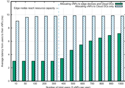
Fig. 3: Comparing the average vNF-to-user E2E latency be-tween edge and Cloud deployments.
in Section II. To show the benefits of running vNFs at the network edge, we compare two scenarios:
1) Cloud-only deployment: vNFs are only allocated to a set of Cloud DCs (three DCs in our case).
2) Two-tier edge deployment: in addition to the Cloud DCs, all points of presence of the backbone network have equal, but finite amount of computing capabilities to host vNFs. When edge devices run out of resources, vNFs are allocated to the Clouds that are further away, yet incur higher latency from the users.
In this experiment, we have assigned end users to edge locations in a round robin fashion and set a fixed user-to-edge latency of 3 ms, a fair estimation for an average last hop latency based on the studies in [6]. For this experiment, we have assumed 3 vNFs per user (one with real-time, one with near real-time and one with non real-time latency requirement) and assigned computing capabilities to all edge nodes with a total capacity of 1000 vNFs (ca. 40 vNFs per edge node).
In Figure 3, we show the average latency from users to their vNFs. The Cloud-only deployment gives an average latency of 10 ms between users and their vNFs, while running vNFs at the edge results in a 3 ms average latency until the edge nodes reach the limits of their capacity and vNFs. When edge nodes run out of resources, the average vNF-to-user E2E latency starts converging to that of the Cloud-only scenario since, from this point onward, vNFs are being allocated to the cloud servers, resulting in longer communication paths. Therefore, placing vNFs at the network edge can result in significantly lower (up to 70% decrease) vNF-to-user E2E latency.
0 200 400 600 800 1000 1200 1400 1600 1800 0 10 20 30 40 50 60 70 80 90 100 Objective function (ms) Time instance t=0 optimal allocation Objective function at t
(a) Deviation from optimal alloca-tion per time instance.
0 1 2 3 4 5 6 0 10 20 30 40 50 60 70 80 90 100 Number of violations Time instance
Number of latency violations caused
(b) Number of latency violations per time instance.
Fig. 4: Deviation from the optimal placement and the number of violations per time instance.
C. Analysing Latency Violations
Since the latency matrix l changes over time (due to changes in link latency and in users’ physical location), the sys-tem deviates from a previously optimal placement over time. This behaviour is shown in Figure 4a, where we highlighted the difference between an old value of the objective function (Eq. 2) and the value of this objective function calculated at every time instance t (a time instance can be e.g., 5 minutes on a production deployment) based on the temporal latency parameters. As shown, successive objective values can deviate between -25% an 200% from each other.
These deviations from a previously optimal allocation can result in latency violations which note that a vNF ni expe-riences higher vNF-to-user E2E latency than the θi threshold used for the previous (optimal) placement, as it is shown in Figure 4b. As it can be seen by looking at Figure 4b and Figure 4a at the same time, while deviations from an optimal placement happen at any time, not all deviations are respon-sible for latency violations (since a deviation can distribute between all users and vNFs not violating any particular vNF-to-user E2E latency requirement). It is important to note that the number of violations counted at different time instances is the key for calculating the optimal time for migration, since we are using its cumulative distribution and mass functions in Eq. 14 asP(L=`)to predict the number of latency violations the system will experience at the next time instance. These properties are unique for the network topology, vNF locations and the physical locations of the users. We envision learning
P(L = `) for a period of time (e.g., 100 time instances) before kicking off the placement scheduler. While in operation, we continuously update P(L =`)based on the experienced violations.
D. Placement Scheduling Using Optimal Stopping Time 1) Basic behaviour: For this experiment, we run the system for 800 time instances which represents 2 days and 18 hours of operations in case 5 minutes is selected for a time instance by the operator. We present the behaviour of our placement scheduling solution described in Section III. As shown in Figure 5a, the system experiences accumulated latency vio-lations towards the latency tolerance threshold Θ set by the operator for the system (or Θ can be set for a subset of users to differentiate QoS received by different groups of users). After some time, just before reaching this threshold,
0% 25% 50% 75% 100% 125% 0 100 200 300 400 500 600 700 800
Number of cumulative violations towards the threshold
Time
Cum. number of violations using optimal stopping time (our solution) Maximum number of violations tolerated Θ
(a) Our scheduler optimises for a new placement avoiding reaching the violation threshold. 0 0.2 0.4 0.6 0.8 1 -1 0 1 2 3 4 5 6 PDF
Number of latency violations Learned (actual) P P based on N(µ = 2.5, σ2 = 0.5)
(b) Distribution of the number of latency violations per time.
Fig. 5: Our proposed scheduler triggers the optimisation just before reaching a latency violation threshold.
0 10 100 1000 10000 0 100 200 300 400 500 600 700 800
Number of cumulative migrations
Time
Migrating every time instance Our scheduler based at optimal stopping time (our solution) Our scheduler using P based on normal distribution Migrating every 100 time instance
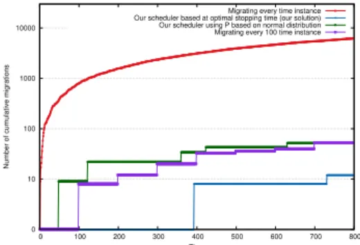
Fig. 6: Comparison of the number of migrations with various migration scheduling strategies.
the system triggers the re-calculation of the placement and performs vNF migrations in order to reach the new latency-optimal location while zeroing the accumulation of latency. As also shown in Figure 5a, the scheduling algorithm is fully adaptive to the number of latency violations experienced by unpredictable latency deviations. As an example, the second migration happens much later from the optimal point than the first one.
It is also important to note that Eq 16 relies onFL(`) = P`
l=0P(L = l) and P(L = `) that are the cumulative
distribution and mass functions of L in (11), respectively. In order to learn P(L = `), we left the system running for 100 time instances (that would mean around 8 hours if 5 minutes is selected for a time instance by the operator) before scheduling the first re-allocation of the placement. This is required, since the optimal stopping is calculated based on the previously-learned distribution of latency violations per time instance P(L=`). It is important to note that the properties of P(L=`)determine when to trigger a migration and it can be in various stages of the system.
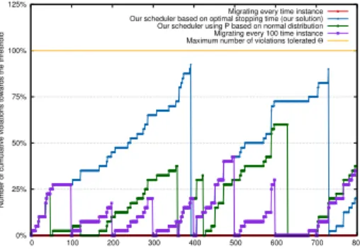
2) Comparison with other placement schedulers: In Fig-ure 6 and FigFig-ure 7, we analyse the trade-off between the number of migrations and the number of latency violations. We have evaluated the following four placement scheduling strategies:
a) Scheduling at every time instance: Scheduling every time instance means that the allocation of vNFs is re-computed and re-arranged at every time instance (e.g., every 5 minutes),
0% 25% 50% 75% 100% 125% 0 100 200 300 400 500 600 700 800
Number of cumulative violations towards the threshold
Time
Migrating every time instance Our scheduler based on optimal stopping time (our solution) Our scheduler using P based on normal distribution Migrating every 100 time instance Maximum number of violations tolerated Θ
Fig. 7: Comparing of the number of cumulative violations with various scheduling strategies.
based on the temporal latency parameters of the network. As shown in Figure 6, migrating vNFs at every time instance re-sults in a 2-3 orders of magnitude higher number of migrations, since every time instance a new placement is calculated and therefore vNF migrations are conducted (vNFs are moved to new devices or new network routes are selected between each user and their vNFs). As expected, this results in zero latency violations at every time instance since vNFs are always at their optimal location, as shown in Figure 7.
b) Scheduling at optimal stopping time using learned
P(L=`): This approach, which is the one we have adopted in this work, minimises the number of migrations while it guarantees that the system never reaches the maximum number of allowed violationsΘ. This solution depends on the learned distribution of latency violations at every time instance which we gathered by leaving the system to run for 100 time instances before scheduling any re-optimisation of the placement. As shown in Figure 6, our strategy re-computes the placement two times and performs only 12 vNF migrations while, as shown in Figure 7, it got very close, reaching 87% of the latency violations threshold of the system. From the Figures we can also observe that our scheduler can eliminate at least 76.9% and up to 94.8% of the vNF migrations compared to other schedulers.
c) Scheduling a new placement usingP(L=`) follow-ing the Normal distribution: The distribution of experienced latency violations is a key parameter in our model, as shown in Eq. 16. As presented before, in order to get the best result, we advise a learning phase for the system, where the
P(L = `) distribution of the latency violations is learned. In this experiment, however, instead of using the learned
P(L=`)based on previous observations, we assume that the latency violations in the system follow a Normal distribution
N(2.5,0.5) and therefore we used our optimal stopping time scheduler with this fixed distribution instead of the learned distribution. The difference between the two distributions is shown in Figure 5b. While assuming a Normal distribution for
P(L=`) eliminates the need for learning, it initiates a new placement much sooner than our scheduler using the learned distribution of latency violations as shown in Figures 6 and 7. In our case, re-calculation of the placement is scheduled sooner as the probabilities of getting high number of latency violations at a time instance are higher compared to the learned distribution. While this results in a sub-optimal solution, an
operator could start with such approximated distribution for
P(L=`)and adapt the distribution of latency violations over time to the actual experienced latency violations.
d) Scheduling a new placement at fixed periodic in-tervals: This strategy initiates vNF migrations at set time intervals, independent of the number of latency violations experienced before. This is the most basic scheduling strategy a network operator could implement by, e.g., initiating a network configuration batch-job re-allocating vNFs at the same time ev-ery night. Looking at the number of migrations in Figure 6, this strategy results in a moderate number of migrations compared to other strategies. Also, as shown in Figure 7, if the selected time interval is short enough (e.g., every 100 time instances), the cumulative number of latency violations never reaches the threshold. However, it is important that this strategy does not depend on P(L=`), the latency violations experienced and therefore does not adhere to the latency violation thresholdΘ, meaning that a long interval (e.g., every 500 time instances in our case) would result in violating the threshold. In fact, our solution tackles the problem of systematically selecting the right time to re-compute the placement without manual and constant tuning from the operator.
As shown, each scheduler has a distinct behaviour. While scheduling the re-optimisation of the placement every time instance results in zero latency violations, it requires many vNF migrations, performed at every time instance. On the contrary, migrating periodically results in fewer migrations but it requires a constant tuning from an operator to select the right time for re-optimisation of the placement. Our solution using optimal stopping theory selects the right time for placement just by looking at the previously experiences latency violations noted in P(L = `). In order to show the importance of
P(L=`), we have also presented a scheduler that estimates the latency distribution and does not learn it.
V. RELATED WORK
Moving intelligence from traditional servers at the centre of the network to the network edge is gaining significant attention from both the research and the industry communities, as discussed in [17] and [4]. The term ”fog computing” [18] has been defined to offload computation to nearby devices (forming a ”fog”), while the ”multi-access edge computing (MEC)” [3] by ETSI advocated the use of edge servers to run customised services for users. Already presented industrial solutions promoting the edge include ADVA’s One Network Edge offering that provides a comprehensive range of edge services running on specific, enhanced, yet simplified packet forwarding devices. In research, the benefits of an edge in-frastructure have been explored from various angles. As an example, the authors in [19] have presented the prominent work on ”cloudlets” that bring Cloud to the mobile users by exploiting computing services in their spatial vicinity. As another example, the authors of [4] present how one can use container network functions at the network edge to provide services such as, e.g., DDoS protection and remote network troubleshooting.Our work contributes to this fieldby presenting a dynamic, latency-based vNF placement that can be used by the aforementioned technologies to support latency-sensitive applications.
With the rise of 5G networks, ultra-low and predictable end-to-end latency is becoming increasingly important as the key enabler for many new and visionary applications. Achiev-ing ultra-low latency has been attempted at various points of the networking stack, from the OS kernel [20] to 5G millimeter-wave cellular networks [21]. In contrast to these works, to the best of our knowledge, our approach is the first to investigate an end-to-end latency optimisation problem from a wider, high-level perspective, and optimised the physical lo-cation of edge vNFs based on real-time latency measurements on the links and the number of latency violations encountered. Orchestrating and managing vNFs in different NFV infras-tructures has been a popular research topic and it is often related to the traditional Virtual Machine (VM) placement problem. As a prominent example for vNF placement, in [7], the authors have presented VNF-P, a generic model for efficient placement of virtualized network functions. Some other works have also taken latency as a parameter in vNF orchestration, similar to what we are proposing in this paper. As an example, in [13] the authors presented a latency-aware composition of virtual network functions that identifies the order and place-ment location of vNF chains. In contrast to their optimisation
which targets DCs, in this paper we have formulated a novel placement model for a distributed network edge and have let the placement to follow latency trends dictated by the SLA violations allowed.
VI. CONCLUSIONS
In this paper, we advocated that in order to sustain low end-to-end latency from users to their vNFs in a contin-uously changing network environment, one has to migrate vNFs to optimal locations numerous times during the life of a NFV system. We have therefore defined an optimal placement model with a dynamic scheduler that adapts to changes in network latency over the infrastructure and re-evaluates the placement of vNFs according to the number of latency violations permitted in the system. We have evaluated the proposed vNF orchestrator using a simulated nation-wide network topology with real-world latency characteristics and users running multiple latency-sensitive vNFs.
Our results show that our dynamic vNF placement sched-uler reduces the number of migrations by 94.8% and 76.9% compared to a scheduler that runs every time instance and one that would periodically trigger vNF migrations to a new optimal placement, respectively. By applying such dynamic and latency-aware scheduling on top of a vNF placement optimisation, operators can reduce network utilisation and min-imise service interruption while meeting the service guarantees to subscribed users.
ACKNOWLEDGEMENTS
The work has been supported in part by the UK Engineer-ing and Physical Sciences Research Council (EPSRC) projects EP/L026015/1, EP/N033957/1, and EP/P004024/1, and by the European Cooperation in Science and Technology (COST) Action CA 15127: RECODIS – Resilient communication and services. This research is funded by the EU H2020 GNFUV Project/Action RAWFIE-OC2-EXP-SCI (Grant No. 645220), under the EC FIRE+ initiative.
REFERENCES
[1] A. Osseiran, F. Boccardi, V. Braun, K. Kusume, P. Marsch, M. Maternia, O. Queseth, M. Schellmann, H. Schotten, H. Taokaet al., “Scenarios for 5g mobile and wireless communications: the vision of the metis project,”IEEE Communications Magazine, vol. 52, no. 5, pp. 26–35, 2014.
[2] R. Cziva and D. P. Pezaros, “On the latency benefits of edge nfv,” in
Proceedings of the ANCS. Piscataway, NJ, USA: IEEE Press, 2017, pp. 105–106.
[3] Y. C. Hu, M. Patel, D. Sabella, N. Sprecher, and V. Young, “Mobile edge computing - a key technology towards 5g,” ETSI White Paper 11, 2015.
[4] R. Cziva and D. P. Pezaros, “Container network functions: Bringing nfv to the network edge,”IEEE Communications Magazine, vol. 55, no. 6, pp. 24–31, 2017.
[5] J. G. Andrews, S. Buzzi, W. Choi, S. V. Hanly, A. Lozano, A. C. Soong, and J. C. Zhang, “What will 5g be?”IEEE Journal on selected areas in communications, vol. 32, no. 6, pp. 1065–1082, 2014.
[6] C. Pei, Y. Zhao, G. Chen, R. Tang, Y. Meng, M. Ma, K. Ling, and D. Pei, “Wifi can be the weakest link of round trip network latency in the wild,” inINFOCOM 2016. IEEE, 2016, pp. 1–9.
[7] H. Moens and F. De Turck, “VNF-P: A model for efficient placement of virtualized network functions,” inCNSM. IEEE, 2014, pp. 418–423. [8] M. F. Bari, S. R. Chowdhury, R. Ahmed, and R. Boutaba, “On orches-trating virtual network functions,” inCNSM, 2015 11th International Conference on. IEEE, 2015, pp. 50–56.
[9] A. Gember-Jacobson, R. Viswanathan, C. Prakash, R. Grandl, J. Khalid, S. Das, and A. Akella, “Opennf: Enabling innovation in network func-tion control,” in ACM SIGCOMM Computer Communication Review, vol. 44, no. 4. ACM, 2014, pp. 163–174.
[10] G. Peskir and A. N. Shiryaev, Optimal stopping and free-boundary problems. Springer Science & Business Media, 2006.
[11] M. Chiosiet al., “Network Functions Virtualisation: An Introduction, Benefits, Enablers, Challenges & Call for Action,” ETSI White paper, 2012.
[12] R. Cziva, S. Jouet, and D. P. Pezaros, “GNFC: Towards Network Function Cloudification,” inProc. of 2015 IEEE NFV-SDN, Nov 2015, pp. 142–148.
[13] B. Martini, F. Paganelli, P. Cappanera, S. Turchi, and P. Castoldi, “Latency-aware composition of virtual functions in 5g,” inProceedings of the 2015 1st IEEE Conference on Network Softwarization (NetSoft), April 2015, pp. 1–6.
[14] F. B. Jemaa, G. Pujolle, and M. Pariente, “Qos-aware vnf placement op-timization in edge-central carrier cloud architecture,” inGLOBECOM, Dec 2016, pp. 1–7.
[15] A. Q. Frank and S. M. Samuels, “On an optimal stopping problem of gusein-zade,” Stochastic Processes and their Applications, vol. 10, no. 3, pp. 299–311, 1980.
[16] R. Cziva, C. Lorier, and D. P. Pezaros, “Ruru: High-speed, flow-level latency measurement and visualization of live internet traffic,” in
Proceedings of the SIGCOMM Posters and Demos. ACM, 2017, pp. 46–47.
[17] A. Manzalini and R. Saracco, “Software networks at the edge: A shift of paradigm,” in 2013 IEEE SDN for Future Networks and Services (SDN4FNS), Nov 2013, pp. 1–6.
[18] F. Bonomi, R. Milito, J. Zhu, and S. Addepalli, “Fog computing and its role in the internet of things,” inProceedings of the first edition of the MCC workshop on Mobile cloud computing. ACM, 2012, pp. 13–16. [19] T. Verbelen, P. Simoens, F. De Turck, and B. Dhoedt, “Cloudlets: Bringing the cloud to the mobile user,” inProceedings of the third ACM workshop on Mobile cloud computing and services. ACM, 2012, pp. 29–36.
[20] R. Kapoor, G. Porter, M. Tewari, G. M. Voelker, and A. Vahdat, “Chronos: predictable low latency for data center applications,” in
Proceedings of the Third ACM Symposium on Cloud Computing. ACM, 2012, p. 9.
[21] R. Ford, M. Zhang, M. Mezzavilla, S. Dutta, S. Rangan, and M. Zorzi, “Achieving ultra-low latency in 5g millimeter wave cellular networks,”