Constrained School Choice: An Experimental Study
∗Caterina Calsamiglia† Guillaume Haeringer‡ Flip Klijn§
November 17, 2008
Abstract: The literature on school choice assumes that families can submit a preference list over all the schools they want to be assigned to. However, in many real-life instances families are only allowed to submit a list containing a limited number of schools. Subjects’ incentives are drastically affected, as more individuals manipulate their preferentes. Including a safety school in the constrained list explains most manipulations. Competitiveness across schools play an important role. Constraining choices increases segregation and affects the stability and effi-ciency of the final allocation. Remarkably, the constraint reduces significantly the proportion of subjects playing a dominated strategy.
JEL classification: C72, C78, D78, I20
Keywords: school choice, matching, experiment, Gale-Shapley, top trading cycles, Boston mech-anism, efficiency, stability, truncation, truthtelling, safety school
∗We thank Yan Chen, Fuhito Kojima, Charles Mullin, Muriel Niederle, David Reiley, Ludovic Renou, Tayfun
S¨onmez, Utku ¨Unver and participants of the Caltech SISL Mini-Conference on Matching for helpful discussions, and Sebastian Bervoets for research assistance. The authors acknowledge support of Barcelona GSE Research Network and of the Government of Catalonia, Ram´on y Cajal contracts of the SpanishMinisterio de Ciencia y Tecnolog´ıa, the SpanishPlan Nacional I+D+I (SEJ2005-01481, SEJ2005-01690 and FEDER), theGeneralitat de Catalunya (SGR2005-00626) and theConsolider-Ingenio 2010 (CSD2006-00016) program. This paper is part of the Polarization and Conflict Project CIT-2-CT-2004-506084 funded by the European Commission-DG Research Sixth Framework Program. This article reflects only the authors’ views and the Community is not liable for any use that may be made of the information contained therein.
†Departament d’Economia i d’Hist`oria Econ`omica, Universitat Aut`onoma de Barcelona, Spain; e-mail:
‡Departament d’Economia i d’Hist`oria Econ`omica, Universitat Aut`onoma de Barcelona, Spain; e-mail:
§Institute for Economic Analysis (CSIC), Spain; e-mail:
1
Introduction
School choice programs offer families a say in the assignment of their children to public schools. Inspired by the successes in the design of markets for physicians (Roth and Peranson, 1999), law clerks (Avery, Jolls, Posner and Roth, 2001) and others, the matching literature has shown to be able to propose concrete solutions to design school choice mechanisms —Abdulkadiro˘glu and S¨onmez (2003).1
Recent works on the implementation of school choice mechanisms have raised new issues for which the literature had little to say but appeared to be important aspects of school choice design. For instance, the problem of breaking ties in case of indifferences, somehow overlooked by the theoretical literature until a few years ago, proved to be far more complex and important than originally thought (Erdil and Ergin, 2008).2
In this paper we focus on another seemingly unimportant aspect of school choice mechanisms which turns out to have strong effects on their performance. The literature assumes that families can submit a list of all schools that are acceptable for the family. However, in many real-life instances families are only allowed to submit a list containing a limited number of schools. For instance, in the school district of New York City each year more than 90,000 students are assigned to about 500 school programs and parents are asked to elicit a preference list containing a maximum number of schools (currently 12).3
Other examples include college admissions in Spain and Hungary where students cannot submit a choice list containing more than 8 and 4 academic programs, respectively.4
This apparently innocuous restriction is reason for concern. When an individual’s choice is constrained by the number of schools he can include in his choice list, the risk that the mechanisms may exhaust the options listed becomes non-negligible. In particular, if he fears rejection by his most preferred programs, it can be advantageous not to apply to these programs and use the allowed application slots for less preferred programs.5
These
1
See also Abdulkadiro˘glu, Pathak and Roth (2005) and Abdulkadiro˘glu, Pathak, Roth and S¨onmez (2005).
2
See also Abdulkadiro˘glu, Pathak and Roth (fortcoming).
3
Students that are not assigned a seat are asked to elicit a second list containing only schools withvacantseats. The resulting mechanism does not provide the right incentives for truthful behavior of the participants. The pure mechanism, i.e., the mechanism without constraint, would solve this matter. See Abdulkadiro˘glu, Pathak and Roth (2005) for details.
4
In Spain and Hungary colleges are not strategic, for the priority orders are determined by students’ grades. So college admission in these countries is, strictly speaking, akin to school choice.
5
Obviously, if the number of acceptable schools for individuals is smaller than the number of slots in the list there is no problem. However, in case the number of slots is restrictive individuals will have to think out which schools to include and in which order. Abdulkadiro˘glu, Pathak and Roth (2005) report that in New York City about 25% of the students exhausted their list in academic year 2003–2004, which suggests that the constraint was indeed binding for a substantial proportion of students.
decisions are made under uncertainty and therefore ex-ante safe optimal strategies may lead to inefficiencies if individuals do not apply to schools that would have accepted them had they have applied to them. Therefore, imposing a curb on the length of the submitted lists, though having the apparent merit of simplifying matters, may have the perverse effect of forcing participants not to be truthful, and compel them to adopt strategic behavior.6
Also, the literature only provides clear predictions in terms of stability, efficiency and behavior when choice is not constrained.7 Perhaps more important is the fact that when choice is constrained the risk of being unassigned (or assigned to a school one likes very little) makes it less safe for individuals to participate in the market, which may cause market failures.8
The goal of our experimental study is to propose an overhaul of the most prominent match-ing mechanisms when we impose a maximal length of the submittable preference lists. More precisely, we focus on three matching mechanisms: the Boston (BOS), the Student Optimal Stable Matching (SOSM) and the Top Trading Cycles (TTC) mechanisms. These mechanisms (and their variants) are or have been employed or proposed in many US school districts. They are also subject of many theoretic, experimental and empirical studies, virtually all of them assuming the absence of a constraint on the length of submittable preference lists.
Our objective in the experimental analysis is twofold. First, we seek to characterize be-havioral patterns and identify what features in a school choice mechanism govern the observed behavior. Our analysis will not only focus on the algorithms used to match students to schools but also on other aspects of the market, such as the differences in competitiveness across schools, which may be crucial for understanding strategic behavior. The literature has proposed mech-anisms that are strategy-proof when there is no constraint, that is, they induce a game where truth-telling is a dominant strategy. In the constrained game being truthful is not only infeasible but there is also no dominant strategy. We expect though that individuals will strategize and play “safely,” that is, they will try to guarantee themselves a “decent” school according to their preferences.
Our second objective is to scrutinize the outcomes obtained in the school choice games. First we compare the efficiency and stability attained across the various mechanisms. Stability, as argued by Roth (1991), plays an important role in the viability of matching institutions. Roughly speaking, a matching is stable when for each student all the schools he prefers to the
6
Non-manipulability played an important role in the decision of public school authorities in Boston and New York to change the mechanisms that they employed until recently. See also Abdulkadiro˘glu, Pathak, Roth and S¨onmez (2005) and Abdulkadiro˘glu, Pathak and Roth (2005).
7
Haeringer and Klijn (2008) provide an equilibrium analysis for the constrained setting which makes clear that the predictions from the unconstrained setting do not carry over in a straightforward way.
8
one he is assigned to have their capacity filled with higher priority students. In the unconstrained setting, SOSM is stable and TTC is efficient, but none of the two satisfies both properties since they are known to be incompatible. We hypothesize that the introduction of the constraint will decrease the stability and efficiency exhibited by both SOSM and TTC. Another important aspect we examine is the distribution of students across schools. School choice is indeed one way of enhancing social mixing by allowing parents to apply for a school outside their district. If choice is constrained, and thus the risk of being assigned to an undesirable school is high, asking admission to the district school may become a tempting strategy. This may in turn reduce mobility.9
Through our experiment we want to provide evidence of the existence and strength of this effect.
To this end, we experimentally study the school choice problem using a variant of the exper-imental design initially proposed by Chen and S¨onmez (2006). This design consists of a school choice problem involving 36 subjects (i.e., students) to be assigned to 7 schools, which have 2 different capacities (low and high). Also, to mimic real-life settings, students are assigned to one of 7 districts, each district containing one school. Students in a district are given the highest priority at the school of their district. There are two payoff environments, designed and ran-dom. In the designed environment the low capacity schools and, to a lesser extent, the district school (i.e., the school in the student’s district) are more likely to be among the most preferred schools. In the random environment preferences are uncorrelated. In both environments, all schools are acceptable to all students (i.e., any school seat is better than remaining unassigned). The experiment consists first of collecting preference lists by subjects, then determining schools’ strict priority orderings and finally computing an assignment of students to schools. The final assignment is determined by either of the three mechanisms we focus on: BOS, SOSM and TTC. BOS is one of the most employed mechanisms in practice, and is based on the idea that it is desirable to satisfy students’ top choice as much as possible. As shown by Abdulkadiro˘glu and S¨onmez (2003), achieving this objective comes at a double cost. First, the mechanism gives a strong incentive to not be truthful. Second, the outcome obtained with BOS is likely to be un-stable. In the unconstrained setting, SOSM does not suffer the drawbacks of BOS. Under SOSM it is a dominant strategy to reveal one’s true preferences and it produces a stable assignment (provided that agents submit their true preferences). However, since SOSM is not efficient, a possible alternative is TTC, which is efficient (but not stable) and also maintains truthtelling as a dominant strategy.10
9
See Niederle and Roth (2003) for an account on mobility.
10
Ergin (2002) and Kesten (2006) show that the efficiency of SOSM and the stability of TTC can only be ensured under very restrictive conditions on the schools’ priorities. None of these conditions are satisfied in the
We use Chen and S¨onmez’s (2006) protocol considering two cases, one in which subjects are not constrained by the number of schools they can include in the list, and one in which they cannot submit a list containing more than three schools. This protocol is well suited for our purposes for several reasons. First, the two different payoff environments and the heterogeneity of schools enable us to disentangle the extent to which the payoff structure and the distribution of capacities across schools affect subjects’ behavior. Second, the experiment consists of a one-shot game with incomplete information. Each subject only knows his own payoff table and his district school (the school for which he has the highest priority). A recent experiment study by Pais and Pint´er (2008) shows that, in the unconstrained case, the less information subjects have about others’ payoffs the more likely they are to be truthful for BOS, SOSM and TTC. That is, providing subjects with virtually no information about their opponents’ payoffs represents the least favorable situation to reject that the mechanisms induce truthful behavior. More importantly, the same properties of the game allow us to use a recombinant technique to obtain robust estimates when evaluating the outcomes generated by the different mechanisms. Third, contrary to most real-life mechanisms we do not run an after-market to assign students that are left unassigned among the schools that have not filled their capacities. It is our contention that in real-life settings the cost of not being assigned to one of the schools in the submitted list is very high or higher than the payoff difference we can provide to individuals in our experiment. In our experimental design the only way to mimic such a high costs consists of not running an after-market and leaving unassigned subjects with just their participation fee. By not doing so we would have lowered significantly the cost of not being assigned in the primary market and thus miss the effect thatconstrained choice has on the school choice mechanisms.
Our experimental study aims at contributing to both the behavioral and the matching lit-eratures. From the behavioral perspective our experiment provides evidence of several stylized facts. First, we observe that when individuals are constrained, the risk of being unassigned if they do not pick an appropriate list induces them to “think harder,” that is, to understand better the mechanism and thereby use less often a dominated strategy.11
Second, we observe that subjects that have more to lose, by having their safe option further down in their preferences, are also better optimizers than subjects with more “favorable” prefer-ences, that is, with their district school in one of the three positions in their preferences. In fact, to streamline the analysis we partition the subjects into two samples. The first sample, which we call the high-district sample, contains all the subjects for which the district school is ranked
experimental design we consider.
11
Haeringer and Klijn (2008) show that for SOSM and TTC not respecting the relative order of schools in the choice list is a dominated strategy.
high in their preferences. For these subjects constraining their choices does not affect their incentives to be truthful. Furthermore, they are ensured to obtain a high payoff since their own district school is the easiest to be assigned to in any of the mechanisms. The low-district sample contains the remaining subjects. For them the constraint hampers their prospects and choosing an appropriate strategy is far more complex. In general we observe more signs of optimizing behavior from the low-district subjects than from the high-district subjects.12
Third, we introduce a taxonomy of biases to characterize strategic choices (e.g., altering the relative position of the district school). Not surprisingly, the introduction of a constraint on the choice exacerbates the intensities of the different biases we consider. However, a more startling observation is that which bias is predominant, and whether biases are correlated or not changes with the experimental treatment. We find that the structure of biases does not only differ between the low and high-district samples but also between the constrained and unconstrained settings. This suggests that constraining choice affects the way individuals apprehend the game and thus the way they elaborate their strategic choices.
From the matching literature perspective, our experiment aims at probing the mechanisms when played with and without the constraint on the size of the submittable preference lists. For SOSM and TTC not all subjects use their (weakly) dominant strategy whenever available, for both the constrained case (high-district subjects) and unconstrained case (all subjects). How-ever, we find that many of the non-optimal manipulations are due to the presence of asymmetries in school capacities. This suggests that details such as the differences in competitiveness across schools are important elements influencing individual behavior.
In spite of a loss of predictability of subjects’ behavior in the constrained setting we find that the relative ranking of the mechanisms in terms of efficiency is quite robust.13
That is, TTC outperforms SOSM which in turn is superior to BOS. As for the stability of the assignments obtained, the results are less encouraging. In general, assignments are not stable. The picture becomes clearer if we consider the average number of blocking pairs, which can be interpreted as a measure of discontent or inviability of the market institution. SOSM emerges as the best mechanism since it leads to significantly less blocking pairs than BOS and TTC. Also,
12
Due to the high complexity of the game under consideration it is computationally very difficult to assess the performance of a given strategy. The games under consideration in our experiment involve 36 players, with 260 and 13700 different strategies in the constrained and unconstrained case, respectively. Hence, approaches like
k-level thinking (Costa-Gomes, Crawford and Iriberri, forthcoming) or quantal response equilibrium (McKelvey
and Palfrey, 1995) are not suitable in our case.
13
Recall that in our experiment there is incomplete information. Apart from a recent paper by Ehlers and Mass´o (2007), which links equilibria under complete information with Bayesian equilibria under incomplete in-formation, there are yet no theoretical results that can offer an insight in individuals’ optimal behavior.
constraining choice clearly increases the number of blocking pairs for SOSM (but not for BOS and TTC).
Finally, when investigating the extent to which the three mechanisms can counter the segre-gation in neighborhoods, we observe that more students are assigned to their district school in the constrained setting. However, we observe that segregation rates under SOSM and BOS are not statistically different, but always higher than those under TTC.
The remainder of the paper organized as follows. The school choice problem and the three mechanisms analyzed in this paper are presented in Section 2. In Section 3 we present our main hypotheses. The experimental design is explained in Section 4. Experimental analysis and results are in Section 5. Section 6 concludes.
2
School Choice
A school choice problem (Abdulkadiro˘glu and S¨onmez, 2003) is defined by a set of schools and a set of students, each of which has to be assigned a seat at no more than one school. Each student is assumed to have strict preferences over schools and the option of remaining unassigned. Each school is endowed with a strict priority ordering over students and a fixed capacity of seats. If a student prefers the option of remaining unassigned to being assigned a seat at a given school, then this school is said to be unacceptable for the student. Otherwise, a school is acceptable.
An outcome of a school choice problem is a matching, i.e., an assignment of students to school seats such that each student is assigned at most one seat and each school receives no more students than its capacity. At a given matching, a student is unassigned, or assigned to himself, if he is not assigned a seat in any school. In the context of school choice, schools are institutions serving society and so only the welfare of the students is considered. Hence, a matching is Pareto efficient if there is no matching that gives every student a weakly better assignment and at least one student is strictly better off.
A matching is stable if: (a) it is individually rational, i.e., each student is unassigned or assigned a seat at some acceptable school; (b) it is non wasteful (Balinski and S¨onmez, 1999), i.e., no student prefers a vacant seat to his assigned seat; and (c) there is no justified envy, i.e., there is no student-school pair (i, s) such that i prefers s to his assignment and i has higher priority atsthan some other student who is assigned a seat at s.
A (student assignment) mechanism systematically selects a matching for each school choice problem. A mechanism is stable if it always selects a stable matching. Similarly, an efficient mechanisms is one that always selects a Pareto-efficient matching. Finally, a mechanism is
2.1 Three Competing Mechanisms
In this section we briefly describe the mechanisms that we analize in this paper: the Boston (BOS), the Student Optimal Stable Matching (SOSM), and the Top Trading Cycles (TTC) mechanisms. The three mechanisms work as follows. Each school has a strict priority ordering of the students, usually determined by law (giving priority to students from the same neighborhood, having siblings already in the school, etc.).14
Each student is asked to submit achoice list, i.e., an ordered list of schools. Given the priority ranking and the choice lists the three mechanisms determine the final assignment in the following manner.
From the students’ point of view the mechanisms work identically in the following sense: Roundk, k≥1 [students]: Every student that has not been assigned a school in the previous round applies to the highest ranked available school in his choice list that has not rejected him yet (if there is no such school then the student “applies” to himself).
The three mechanisms differ in who gets rejected by a school:
[BOS ]Round k, k≥1 : Each school assigns seats one at a time to the students that apply to it following its priority order. If the school capacity is or was attained, the school rejects any remaining or future applicants. If a student “applies” to himself, he is assigned to himself.
BOS terminates when all students have been assigned.
[SOSM]Round k, k≥1 : Each school tentatively assigns seats one at a time to the students that apply to it or that were tentatively assigned a seat in a previous round, following its priority order. When the school capacity is attained the school rejects any remaining students that apply to it. If a student “applies” to himself, he is tentatively assigned to himself.
SOSM terminates when no student is rejected. Then the tentative matching becomes final.
[TTC]Roundk, k≥1 : Each school with vacant seats “points” to the student with highest priority among the students that have not been assigned a seat yet. This procedure, together with the above described procedure for the students, induces a cycle or cycles of students and schools. If a student is in a cycle he is assigned a seat at the school he applies to (or to himself if he is in a self-cycle). If a school is in a cycle then its number of vacant seats is decreased by one. If a school has no longer vacant seats then it is no longer available and students that applied to it are rejected.
TTC terminates when all students have been assigned.
We consider two cases: an unconstrained case, where students can submit a list containing
14
all schools, and a constrained case, where students can only submit a choice list that contains a small number of schools. In this case, if the mechanism exhausts one of the choice lists, the corresponding student will be removed from the system and be left unassigned.15
In the unconstrained case SOSM and TTC are strategy-proof, but BOS is not. SOSM is also stable.16
However, it is not Pareto efficient. In contrast, TTC is Pareto efficient, but not stable. BOS is Pareto efficient, but since it is not strategy-proof this does not necessarily mean that it is Pareto efficient with respect to the true preferences.17
Under SOSM and TTC revealing your preferences truthfully up to the district school is a weakly dominant strategy in the unconstrained case. In the constrained case, Haeringer and Klijn (2008) explain that there is no dominant strategy and that for SOSM and TTC reversing the relative true ranking of schools is a dominated strategy.
3
Hypotheses on Behavior and Outcomes
Constraining the number of schools that individuals can include in their choice lists should have an effect on behavior, that is, the properties of the submitted lists, and consequently on the final allocation or outcome of the matching process. In this section we describe which differences we expect between the constrained and the unconstrained setup.
In the constrained case playing truthfully up to the district school will not be feasible if the district school’s rank is larger than the number of schools that may be included in the list, k. The predicted behavior therefore will be different for those individuals with the district school above thek−th position or below. For this reason, it will prove useful to partition the sample of subjects into two sub-samples, the high-district sample and the low-district sample. The high-district sample contains all those subjects for which the district school is one of thekmost preferred schools and the low-district sample contains all the other subjects. For subjects in the high-district sample SOSM and TTC are still non-manipulable, that is, revealing one’s true preferences up to the district school is still a weakly dominant strategy.
3.1 Rationality
An important concern in the actual implementation of matching mechanisms is whether in-dividuals understand the game being played and therefore play rationally, that is, play what
15
In real-life settings unassigned students can usually submit a second list, opting only for schools that have vacant seats.
16
In fact, it always generates the best stable matching for the students.
17
an optimizing agent in this particular setup would play.18
In the unconstrained setup playing truthfully is a weakly dominant strategy, but what can we expect a rational agent to play in the constrained setting? Haeringer and Klijn (2008) explain that there is no dominant strategy and that for SOSM and TTC reversing the relative true ranking of schools is a dominated strategy. In fact, the requirement of not reversing the relative true ranking is only necessary up to the district school since for these two mechanisms if a subject asks for its district school, he will be assigned to it, whichever the schools below the district school are. For BOS, the only irrational behavior one can identify is that of not putting the district school as a first option if it is the truly most preferred school.
In the constrained setting subjects need not only decide the order or ranking of the schools but also which schools to include in the list. Although the problem now may seem more complex, incentives to think hard are also higher, since making the wrong choice may lead the subject to be unassigned. So with this additional incentive we expect individuals to try harder to understand the mechanisms and therefore to observe a higher proportion of individuals not playing a dominated strategy. In other words, we expect a higher proportion of rank preservation in the constrained than in the unconstrained setting.19
Rationality HypothesisFor SOSM and TTC, the proportion of individuals behaving rationally is higher in the unconstrained than in the constrained case.
3.2 Truncated-truthtelling
As described in the last section, both SOSM and TTC are strategy-proof in the unconstrained case, that is, it is a weakly dominant strategy to reveal your true preferences up to the district school. But when we add a constraint individuals in the low-district sample do not have a dominant strategy. We therefore expect subjects not to exhibit truncated truthtelling, that is, not to rank their firstkoptions as in their preferences, but to manipulate and submit a different list.
18
See Abdulkadiro˘glu, Pathak, Roth and S¨onmez (2006) or Pathak and S¨onmez (2008) for details.
19
Another explanation leading to the same results would be that the higher complexity of deciding which schools to includeandhow to rank them causes the students to only think about which schools to include and simply maintain the relative ranking of the true preferences by default. In the case of TTC and SOSM this would lead to the proportion of subjects respecting the original ranking being also higher in the constrained case. But for Boston, the different explanations would lead to different results. If subjects are “thinking harder” they should not necessarily respect the ranking. But if the underlying behavioral explanation was that they focus only on which ones to include and respect the ranking by default we would have that the number of subjects respecting the original ranking should also be significantly larger in the constrained setting. Presumably then, observing the results for the three mechanisms should provide some evidence of what the explanation may be.
For BOS we have that both in the unconstrained and in the constrained setting reporting truthfully is not a dominant strategy. Given that the chances of being admitted in a given school get smaller as we go down the choice list individuals have high incentives to manipulate the submitted lists both in the constrained and the unconstrained case by putting a school for which they have chances of being admitted in the first position.
Truthtelling Hypothesis For SOSM and TTC, the proportion of truncated-truthtelling is higher in the unconstrained than in the constrained case. For BOS, the proportion of truncated-truthtelling does not change significantly from the unconstrained to the constrained case.
3.3 Misrepresentations
To understand what drives the subjects’ strategic choices we consider two types of misrepresen-tations introduced by Chen and S¨onmez (2006): District School Bias (DSB) and Small School Bias(SSB). DSB consists of raising the ranking of the district school in the submitted list (for example, ranking the district school in the 3rd position when it is actually 4th or lower in pref-erences). SSB consists of lowering the position of a more competitive school in the submitted ranking. We will define the biases in the constrained and the unconstrained case in the same way so that measures are comparable among treatments. More precisely, we will look at the behavior regarding the initial k positions in the ranking. Therefore, an individual exhibits a DSB if the district school is below the k−th position in the ranking but appears in the choice list or if the district school is in the firstkpositions but is moved up in the ranking in the choice list. In particular, if an individual in the unconstrained case has the district school rankedk+ 2 in preferences but puts it in the k+ 1−st position in the choice list, the individual will not be considered to exhibit a DSB. Similarly, an individual exhibits a SSB if a competitive school was ranked in the firstkpositions in the original preferences and either has not been included in the choice list or has been included in a lower position than in the original preferences.
Both distortions are a natural reaction to the added risk induced by the constraint. If the chances of being unassigned are high, it is very likely that subjects secure their prospects by raising the relative rank of the district school and lowering that of the most competitive schools. While this is very clear for the subjects in the low-district sample, there is no reason for this to happen for the high-district sample individuals (nor for the unconstrained case) under SOSM and TTC.
For BOS the difference in incentives from moving to the constrained environment is smaller since there was already a high risk of exhausting the first positions in the list in the unconstrained case. We therefore expect small or no changes in the misrepresentations observed.
Misrepresentation HypothesisFor SOSM and TTC, a higher proportion of individuals ex-hibit a DSB and a SSB in the constrained compared to the unconstrained case. For BOS, the difference should be small.
3.4 Safety School Effect
The Safety School Effect characterizes a safe strategy for an individual under SOSM or TTC. We say that a subject’s choice exhibits aSafety School Effect(SSE) whenever the district school is ranked bellow thek-th position in the preferences but appears in the first k positions in the submitted list. Note that this effect only concerns subjects in the low-district sample. For both SOSM and TTC the district school is a safe option since, if included in the list, the individual is guaranteed one of its seats. So including it secures the individual from being left unassigned. This effect may not be observed for individuals who do not value their district school (have their district school as one of the worst in the original ranking) and therefore, although it is a secure option, it is bad enough for them to want to take risks by including some other more preferred school.
For BOS incentives are not as large, since only including the district school as a first choice guarantees not being left unassigned. In order for that to be a desirable strategy then, it has to be the case that the district school is a very nice option, since the individual is committing to it when putting it as a first option. We therefore expect SSE to be smaller for BOS than for SOSM and TTC.
Safety School Hypothesis For SOSM, TTC and BOS there is an increase in the proportion of individuals exhibiting SSE in the constrained with respect to the unconstrained case. The SSE should be smaller for BOS than for TTC and SOSM.
3.5 Efficiency and Stability
Efficiency in this context will be measured by the mean payoff of subjects in the different mechanisms. As mentioned earlier, in the unconstrained setting TTC is efficient (provided individuals are truthful), meaning that the average payoff is the maximal feasible mean payoff. SOSM on the contrary is not. BOS is efficient with respect to the submitted preferences, but since we expect little truthtelling, the outcome should not be efficient either. We therefore expect TTC to outperform SOSM and BOS in terms of efficiency.
In the constrained case no theoretical predictions can be made, since efficiency of neither mechanisms is guaranteed. But with the high degree of misrepresentation in the three mecha-nisms we do not expect large differences in mean payoffs.
Efficiency Hypothesis The efficiency of SOSM, TTC and Boston will be reduced in the con-strained compared to the unconcon-strained case. The inefficiency of the three mechanisms in the constrained case is similar.
Stability is an important issue when considering the sustainability of a mechanism. It avoids potential law suits or the appearance of “alternative” markets or mechanisms to perform the matching. Stability guarantees that in a matching, for every individual, the schools he prefers to the one he has been assigned to are filled with higher priority students. In the unconstrained setting we know that SOSM is stable as long as subjects are truthful, but TTC and BOS are not. But in the constrained case no relative ranking of the mechanisms with respect to stability can be theoretically predicted.
Therefore, we predict that in the unconstrained case there will be more stability for SOSM than for the other mechanisms. In the constrained case we can only predict that stability in SOSM is reduced for the constrained case with respect to the unconstrained.
Stability Hypothesis SOSM is more stable than TTC or Boston in the unconstrained case. Stability of SOSM in the constrained should be reduced with respect to the unconstrained case.
3.6 Segregation
School choice can potentially reduce the segregation in schools generated by segregation in neighborhoods by allowing individuals to go to schools that are not in their districts.20
In the constrained setting, since individuals ought to exhibit more DSB they are likely to be allocated to their district school more often than in the unconstrained case. This implies that the degree of segregation of neighborhoods and schools will be more similar when the constraint is present. Segregation HypothesisIndividuals will be assigned to their district school more often in the constrained than in the unconstrained case.
4
Experimental Design
In this section we describe the experimental design. For the unconstrained case the experimental design is that of Chen and S¨onmez (2006). For the constrained case we allow subjects to submit a preference list of up to 3 schools, thereby mimicking the constraint we find in many real-life situations of school choice. Our goal is to obtain a clear-cut and self-contained comparison
20
See Niederle and Roth (2003) for empirical evidence about the mobility generated by a centralized mechanism in the gastroenterology market.
between the two experimental setups that facilitates the identification of the consequences of the restriction on strategic behavior and outcomes.
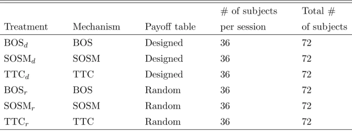
We use a 3 ×2×2 design: each of the three mechanisms is examined in a designed en-vironment as well as a random enen-vironment, and in a constrained and unconstrained setting. For each of the six treatments, two independent sessions were carried out. Table 1 summarizes the main features of the experimental sessions. For each mechanism and for each environment, we conducted by hand two independent sessions between May and November 2006 and in May and June 2008 for the constrained and unconstrained cases, respectively. For each mechanism, payoff environment and case (constrained or unconstrained) one session was ran at the Univer-sitat Aut`onoma de Barcelona and one at the Universitat Pompeu Fabra, and students from a wide range of disciplines attended (economics, psychology, humanities, etc.). Altogether, 864 students participated in the experiments, and the average payoff was e11.8 (not including the e3 participation fee).
# of subjects Total #
Treatment Mechanism Payoff table per session of subjects
BOSd BOS Designed 36 72
SOSMd SOSM Designed 36 72
TTCd TTC Designed 36 72
BOSr BOS Random 36 72
SOSMr SOSM Random 36 72
TTCr TTC Random 36 72
Table 1: Features of experimental sessions for both the constrained and unconstrained setting In each session, there are 36 students and 36 school seats across seven schools. There are three seats at each of the schools A and B, and six seats at each of the schools C, D, E, F and G. Students 1–3 live within the school district of school A, students 4–6 live within the school district of school B, students 7–12 live within the school district of school C, students 13–18 live within the school district of school D, students 19–24 live within the school district of school E, students 25–30 live within the school district of school F and students 31–36 live within the school district of school G.
Schools’ priorities are obtained as follows. We first generate a random order of all students. For each school, the students living in the district of that school are put in the highest position of the priority order of the school, in the order given by the random draw. The other students are
then ranked below, following again the order of the random draw. For instance, if the random draw is 1, 2, . . . , 35, 36, then the priority order of, say, school C is 13, 14, . . . , 18, 1, 2,. . . , 12, 19, 20, . . . , 36.
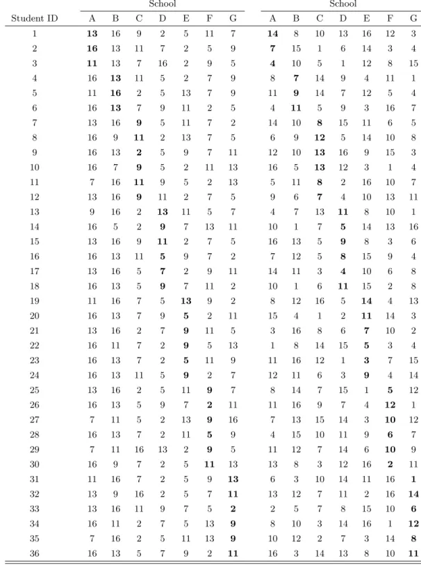
As for the students’ preferences, we consider two payoff environments, designed and random. The designed environment builds on three important real-life factors: a school’s quality, its proximity, and a random factor.21
Based on the induced rankings, the payoff to be received by each participant when assigned to a given school are determined. Payoffs are presented on the left-hand side of Table 2. The random environment is used to check the robustness to changes in the correlation in preferences. Payoffs for the random environment are presented on the right-hand side of Table 2. Boldfaced numbers in the table indicate that the participant lives within the school district of that school.
All three mechanisms were implemented as one-shot games of incomplete information. Each subject knows his own payoff table, but not the other participants’ payoff tables. He also knows that different participants might have different payoff tables. Each session consists of one round only. The sessions last approximately 45 minutes, with the first 20–25 minutes being used for instructions. In addition to the earnings from the experiment, each subject also receives a participation fee ofe3. 22
In the experiment, each participant is randomly assigned an ID number and is seated in a chair in a classroom. The experimenter reads the instructions aloud. Subjects are allowed to ask questions, which are answered in public. Subjects are then given 15 minutes to read the instructions again at their own pace and to make their decisions. Next, the experimenter collects the decisions and asks a volunteer to draw numbers out of an urn, which generates the random order. The experimenter then introduces the subjects’ decisions and the random order in a computer program with the appropriate algorithm to compute the assignment, announces the results, and hands out the corresponding payments to the subjects.
5
Results
When analyzing the data we consider different samples. The “full sample” consists of all subjects. The “low-district sample” consists only of the subjects for whom the district school is ranked 4th or lower in their true preferences. The size of the low-district school varies for the designed and the random environments. In the former case there are 42 subjects and in the latter 44.
21
See Chen and S¨onmez (2006) for details on the design of the rankings and monetary payoffs.
22
We used the exchange rate 1:1 of dollar:euro to convert the monetary payoffs from Chen and S¨onmez (2006) into euros.
Designed payoffs Random payoffs School School Student ID A B C D E F G A B C D E F G 1 13 16 9 2 5 11 7 14 8 10 13 16 12 3 2 16 13 11 7 2 5 9 7 15 1 6 14 3 4 3 11 13 7 16 2 9 5 4 10 5 1 12 8 15 4 16 13 11 5 2 7 9 8 7 14 9 4 11 1 5 11 16 2 5 13 7 9 11 9 14 7 12 5 4 6 16 13 7 9 11 2 5 4 11 5 9 3 16 7 7 13 16 9 5 11 7 2 14 10 8 15 11 6 5 8 16 9 11 2 13 7 5 6 9 12 5 14 10 8 9 16 13 2 5 9 7 11 12 10 13 16 9 15 3 10 16 7 9 5 2 11 13 16 5 13 12 3 1 4 11 7 16 11 9 5 2 13 5 11 8 2 16 10 7 12 13 16 9 11 2 7 5 9 6 7 4 10 13 11 13 9 16 2 13 11 5 7 4 7 13 11 8 10 1 14 16 5 2 9 7 13 11 10 1 7 5 14 13 16 15 13 16 9 11 2 7 5 16 13 5 9 8 3 6 16 16 13 11 5 9 7 2 7 12 5 8 15 9 4 17 13 16 5 7 2 9 11 14 11 3 4 10 6 8 18 16 13 5 9 7 11 2 10 1 6 11 15 2 8 19 11 16 7 5 13 9 2 8 12 16 5 14 4 13 20 16 13 7 9 5 2 11 15 4 1 2 11 14 3 21 13 16 2 7 9 11 5 3 16 8 6 7 10 2 22 16 11 7 2 9 5 13 1 8 14 15 5 3 4 23 16 13 7 2 5 11 9 11 16 12 1 3 7 15 24 16 13 11 5 9 2 7 12 11 6 3 9 4 14 25 13 16 2 5 11 9 7 8 14 7 15 1 5 12 26 16 13 5 9 7 2 11 11 16 9 7 4 12 1 27 7 11 5 2 13 9 16 7 13 15 14 3 10 12 28 16 13 7 2 11 5 9 4 15 10 11 9 6 7 29 7 11 16 13 2 9 5 11 12 7 14 6 10 9 30 16 9 7 2 5 11 13 13 8 3 12 16 2 11 31 11 16 7 2 5 9 13 6 3 10 14 11 16 1 32 13 9 16 2 5 7 11 13 12 7 11 2 16 14 33 13 16 11 9 7 5 2 2 5 7 8 15 10 6 34 16 11 2 7 5 13 9 8 10 3 14 16 1 12 35 7 16 2 5 11 13 9 10 12 2 7 3 14 8 36 16 13 5 7 9 2 11 16 3 14 13 8 10 11
The subjects that are not in the low-district sample conform the “high-district sample,” i.e., the subjects for whom the district school is ranked 3rd or higher in their true preferences. The reason for doing this is that the predicted behavior for the two samples is different. In particular, the high district sample has truncated truthtelling as a weakly dominant strategy but the low district sample does not and has high incentives to strategize.
5.1 Rationality
Table 3 displays the proportion of subjects preserving the original ranking, that is, behaving rationally for the case of TTC and SOSM.
Constrained Unconstrained t-stat p-value
BOSd 34.7 37.5 0.35 0.37 BOSr 37.5 44.4 0.84 0.2 SOSMd 95.8 73.6 3.87 .0001 SOSMr 91.7 81.9 1.73 .043 TTCd 93.1 84.7 1.59 .057 TTCr 90.3 88.9 0.27 .4
Table 3: Preserving original ranking — full sample
As expected, we observe that the proportion of individuals respecting the original ranking for TTC and SOSM in the constrained environment is significantly higher than in the unconstrained environment. This is not true for BOS. This suggests that higher incentives to not make a mistake induce subjects to “think harder” and behave more rationally, which in the case of TTC and SOSM implies preserving the ranking.23
When comparing TTC and SOSM there are no significant differences in the constrained case, but in the unconstrained case TTC exhibits a significantly higher proportion of individuals preserving the ranking.24
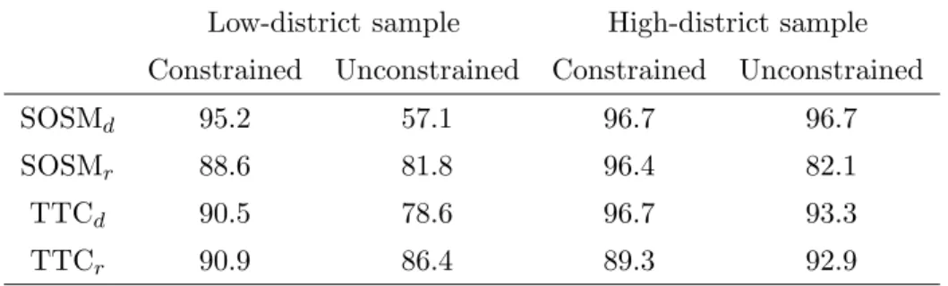
Table 4 presents the data on rationality for SOSM and TTC split out according to the high and low-district school samples. The main difference that can be observed for the unconstrained case is that subjects in the high-district sample are less irrational than subjects in the low-district sample. Also in general the high-low-district sample is more rational, but this may be due
23
For BOS this is not the case, which leads us to conclude that the alternative behavioral explanation introduced in Footnote 19 is not the relevant underlying phenomenon.
24
An argument that has been raised is that the complexity may make the mechanism harder to manipulate. TTC is more complex and therefore may be harder to manipulate.
to the fact that for high-district subjects it is more “difficult” to violate rationality (reversal of first or of first two schools) than for low-district subjects (reversal of first three schools).
Low-district sample High-district sample
Constrained Unconstrained Constrained Unconstrained
SOSMd 95.2 57.1 96.7 96.7
SOSMr 88.6 81.8 96.4 82.1
TTCd 90.5 78.6 96.7 93.3
TTCr 90.9 86.4 89.3 92.9
Table 4: Rationality — high and low district samples
More importantly, it turns out that the lack of rationality is mainly due to the small schools. The violation of rationality for TTC and SOSM systematically concerns only schools A and B. As shown in Table 5, if we consider the relative ranking of all schools up to the district school except schools A and B we find that under TTC and SOSM all subjects respect the original relative ranking. This explains why we observe for the low-district sample (Table 4) a higher proportion of subjects behaving irrationally in the unconstrained setting for the designed compared to the random environment. In the designed environment all subjects have one of the small schools as one of their three most preferred schools, while in the random environment only 52 out of 72 do. That is, the source of irrationality is more present in the designed than in the random environment. In the constrained case although the differences go in the opposite direction they are very small. For BOS we find that competitiveness, or in this case size of the school, is not fully determining individual’s manipulation.
Constrained Unconstrained
Designed Random Designed Random
BOS 63.9 56.9 66.7 58.3
SOSM 100 100 100 100
TTC 100 100 100 100
Table 5: Rationality ignoring small schools — full sample
Distortions of preferences in the constrained setting, which concern the ranking of small schools, are not significantly different for the designed and the random environment. This suggests that what drives this effect is the asymmetry in school capacities, and not the fact that the small schools generally give a higher payoff. This is due to the fact that students do not
know whether preferences are correlated or not, and therefore need not necessarily infer that A and B are the most wanted schools.
5.2 Truthtelling
As described in Section 3.2 subjects under TTC or SOSM in the unconstrained setting should be truthful up to their district school. That is, they should play a truncated-truthtelling strategy. But this should not be so in the constrained setting.
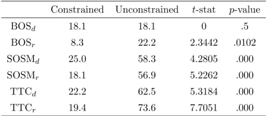
Table 6 displays the percentage of subjects using a truncated-truthtelling strategy in the full sample.
Constrained Unconstrained t-stat p-value
BOSd 18.1 18.1 0 .5 BOSr 8.3 22.2 2.3442 .0102 SOSMd 25.0 58.3 4.2805 .000 SOSMr 18.1 56.9 5.2262 .000 TTCd 22.2 62.5 5.3184 .000 TTCr 19.4 73.6 7.7051 .000
Table 6: Truncated-truthtelling — full sample
Comparing mechanisms in the unconstrained case, BOS has a significantly lower proportion of subjects truthtelling, which is one of the main reasons why Boston Public School authorities were convinced to change from Boston to either SOSM or TTC.25
But note that if a constraint is added the proportion of truthtelling decreases greatly for both TTC and SOSM, making the three mechanisms not statistically different in terms of the amount of truthtelling they exhibit. As conjectured, for BOS there is no increase in truthtelling.
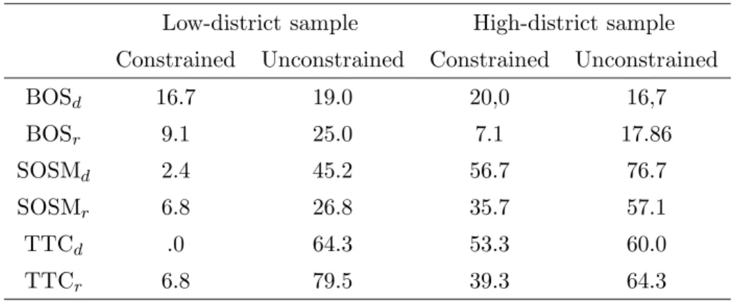
The decrease in truthtelling should be due to truncated-truthtelling not being a dominant strategy, which is only true for the low-district sample. As can be seen in Table 7 the vast major-ity of subjects in the low-district sample do not truthtell in the constrained environment. Note also that in the designed treatment there seems to be slightly less truncated-truthtelling result-ing, as for the rationality case, from the fact that in the designed environment there is a higher proportion of individuals that have small schools in the top three positions in their ranking, which gives them incentives to manipulate their preferences to avoid risks. Surprisingly though, as in the unconstrained case, a very large proportion of subjects from the high-district sample
25
do not truncated-truthtell. In this case, the designed environment leads to more truthtelling, which does not have a clear explanation. The high-district sample seems to generally respond less to the general predictions. They are the group that has less to lose since their secure pay, corresponding to their district school, is high. This again, seems to suggest that having less to lose makes individuals think less, opening the door for irrational behavior.
Low-district sample High-district sample
Constrained Unconstrained Constrained Unconstrained
BOSd 16.7 19.0 20,0 16,7 BOSr 9.1 25.0 7.1 17.86 SOSMd 2.4 45.2 56.7 76.7 SOSMr 6.8 26.8 35.7 57.1 TTCd .0 64.3 53.3 60.0 TTCr 6.8 79.5 39.3 64.3
Table 7: Truncated-truthtelling — high and low-district samples
5.3 Misrepresentations
This section characterizes the main factors driving the low proportion of truncated-truthtelling observed. Tables 8 and 9 report the percentages of subjects having a DSB and SSB, respectively.
Constrained Unconstrained t-stat p-value
BOSd 79.2 68.1 1.5141 .0661 BOSr 76.4 59.7 2.1646 .0160 SOSMd 69.4 15.3 7.8088 .000 SOSMr 77.8 19.4 8.5632 .000 TTCd 68.1 22.2 6.1822 .000 TTCr 73.6 16.6 8.3132 .000
Table 8: District School Bias — full sample
As expected the increase in misrepresentation for TTC and SOSM in the constrained case can be explained by a larger number of subjects pushing the district school up in the submitted list and by lowering the position of small schools, which in this framework are the most competitive schools. For BOS, however, these differences are not always significant, as were the rates of truncated truthtelling. Also, the degree of DSB and SSB is significantly lower for TTC and
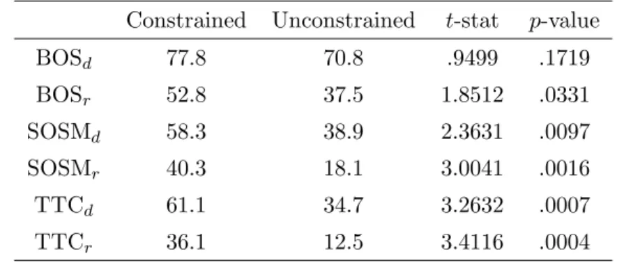
Constrained Unconstrained t-stat p-value BOSd 77.8 70.8 .9499 .1719 BOSr 52.8 37.5 1.8512 .0331 SOSMd 58.3 38.9 2.3631 .0097 SOSMr 40.3 18.1 3.0041 .0016 TTCd 61.1 34.7 3.2632 .0007 TTCr 36.1 12.5 3.4116 .0004
Table 9: Small School Bias — full sample
SOSM than for BOS in the unconstrained case, but not in the constrained case. Although there are some differences between the designed and random environment, none of them are significant.
When considering the high and low-district samples separately (Tables 10 and 11) we ob-serve that for the low-district sample there is a considerable increase in the DSB obob-served and, although smaller, a considerable increase in the SSB. For the high-district sample we see that the increase of both types of misrepresentations is smaller, especially for SSB, where the differences are not significant.
Low-district sample High-district sample
Constrained Unconstrained Constrained Unconstrained
BOSd 81.0 57.1 76.7 83.3 BOSr 75.0 50.0 78.6 75.0 SOSMd 90.5 11.9 40.0 20.0 SOSMr 88.6 18.2 60.7 21.4 TTCd 85.7 14.3 43.3 33.3 TTCr 88.6 9.1 50.0 28.6
Table 10: District School Bias — high and low-district samples
To complete our identification of preference patterns that drive the two main misrepresenta-tions (DSB and SSB) we provide in Table 12 a decomposition of DSB and SSB, separating the subjects’ choices that exhibit only DSB, only SSB and both DSB and SSB. This will shed light on whether DSB and SSB are correlated or not, and if so, under which circumstances.
The most striking observation that can be made from Table 12 is that in the low-district sample DSB is predominant in the constrained case, while it is SSB in the unconstrained case
Low-district sample High-district sample Constrained Unconstrained Constrained Unconstrained
BOSd 76.2 66.7 80.0 76.7 BOSr 59.1 40.0 42.9 32.1 SOSMd 71.4 50.0 40.0 23.3 SOSMr 50.0 20.5 25.0 14.3 TTCd 73.8 33.3 43.3 36.7 TTCr 45.5 11.4 21.4 14.3
Table 11: Small School Bias — high and low-district samples
Low-district sample High-district sample
Constrained Unconstrained Constrained Unconstrained
1 2 3 1 2 3 1 2 3 1 2 3 BOSd 73.8 7.1 2.4 42.3 14.3 23.8 70.0 6.7 10.0 76.7 6.7 0.0 BOSr 52.3 22.7 6.8 27.3 22.7 13.6 32.1 46.4 10.7 28.6 46.4 7.1 SOSMd 64.3 26.2 7.1 9.5 2.4 40.5 36.7 3.3 3.3 20.0 0.0 6.7 SOSMr 47.7 40.9 2.3 9.1 9.1 11.4 21.4 39.3 3.6 7.1 14.3 7.1 TTCd 59.5 26.2 14.3 11.9 2.4 21.4 43.3 0.0 0.0 30.0 3.3 6.7 TTCr 45.5 43.2 0.0 6.8 2.3 4.5 21.4 28.6 0.0 17.9 10.7 10.7
Table 12: Decomposition of biases: (1) DSB and SSB; (2) DSB only; (3) SSB only (especially for the designed environment). This is not the case for the high-district sample, for we seldom observe SSBwithout DSB. Another interesting feature for the high-district sample is the difference between the random and designed environment. When payoffs are not correlated most of the misrepresentations are done through DSB or DSBand SSB, while in the designed environment DSB and SSB are much more correlated.
These results suggests that the constraint significantly affects how subjects elaborate their strategies. The district school becomes focal in the constrained case and significantly less so in the unconstrained case.
5.4 Safety School Effect
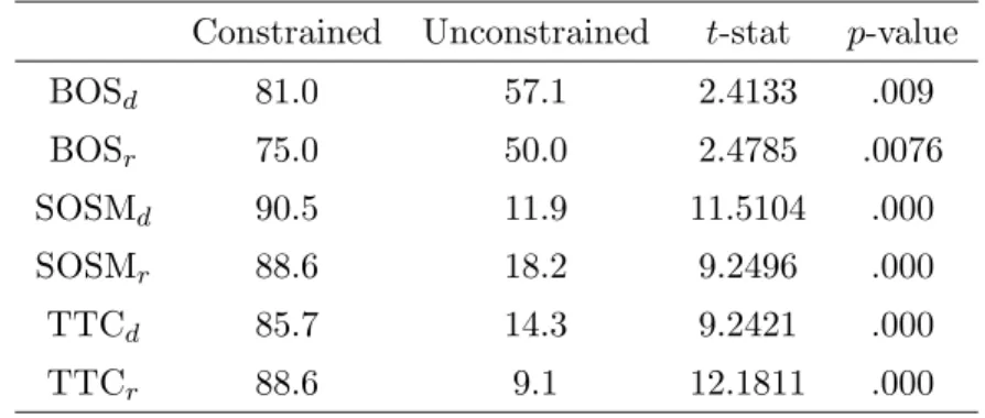
Table 13 displays the proportion of subjects’ choices exhibiting SSE for each of the treatments. As expected, for all three mechanisms we observe a high proportion of subjects exhibiting
Constrained Unconstrained t-stat p-value BOSd 81.0 57.1 2.4133 .009 BOSr 75.0 50.0 2.4785 .0076 SOSMd 90.5 11.9 11.5104 .000 SOSMr 88.6 18.2 9.2496 .000 TTCd 85.7 14.3 9.2421 .000 TTCr 88.6 9.1 12.1811 .000
Table 13: Safety School effect — full sample
the safety school effect for the constrained case. The differences between the constrained and unconstrained cases are highly significant even for the Boston mechanism.
Note that Table 13 and Table 10 for the low-district sample are identical. For the constrained case they are identical by definition. For the unconstrained case it implies that the move upward in the ranking of the district school for subjects in the low district sample is always to one of the first three positions. The first three positions seem to be focal to most subjects, which ex-post could have justified pickingk= 3 as the constraint.
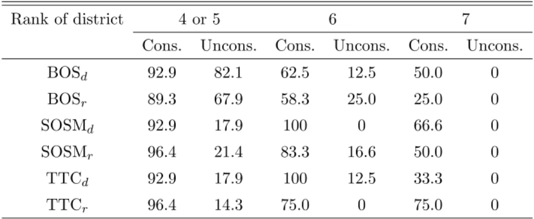
Table 14 shows the percentage of subjects exhibiting SSE classified by the rank of the dis-trict school in their preferences. In the unconstrained case, if the disdis-trict school is ranked 5th or higher there is still a non-negligible proportion of subjects exhibiting a SSE, but this percentage drops when we focus on subjects with the district school in the 6th position, and goes to 0 when the district school is the worse school (in the unconstrained case the worse school’s payoff is guaranteed, and subjects understand that). For the constrained case the SSE is extremely high whenever the district school ranks 5th or higher in the preferences. We observe a considerable decline when the district school is the least desirable school, but the proportion is still surpris-ingly high.26
Even if the school gives them a close to 0 payoff still half of the subjects want to protect themselves from the 0 payoff by including the district school in the choice list instead of a considerably more desirable school. Overall then, the SSE seems to be extremely large for most of the subjects, except for those subjects for which the district school is the worst school.
26
There are 6 and 4 subjects ranking the district school 7th in their preferences in the designed and random environments, respectively. When the district school is ranked 6th in the preferences the sample size is 8 and 12 for the designed and random environments, respectively. There are 28 subjects ranking the district school either 4th or 5th in their preferences for both the designed and random environments.
Rank of district 4 or 5 6 7
Cons. Uncons. Cons. Uncons. Cons. Uncons.
BOSd 92.9 82.1 62.5 12.5 50.0 0 BOSr 89.3 67.9 58.3 25.0 25.0 0 SOSMd 92.9 17.9 100 0 66.6 0 SOSMr 96.4 21.4 83.3 16.6 50.0 0 TTCd 92.9 17.9 100 12.5 33.3 0 TTCr 96.4 14.3 75.0 0 75.0 0
Table 14: Decomposition of the Safety School Effect — full sample 5.5 Efficiency and Stability
5.5.1 The Recombinant Technique
To compare efficiency across mechanisms and environments we employ mean payoffs. For sta-bility we look at the number of stable matchings and at the number of students that form part of a blocking pair in the final assignment.27
Since we have two identical sessions for each treat-ment in principle we only have two observations to make claims on relative performance of the mechanisms. But thanks to the fact that the two identical sessions for each treatment are of a one-shot, incomplete information game we can assume that the behavior of each individual in the two sessions is independent of the particular distribution of the 72 subjects over the two sessions. That is, the behavior of a particular subject does not depend on the particular colleagues in the session and therefore we can assume that his behavior would have been identical if the group of subjects he played against was different. We exploit this fact to obtain more information on what the possible outcomes of the mechanisms could have been. Potentially we could construct 236
different virtual sessions with the 72 individuals from the two sessions. However, to avoid this computational impossibility we recur just as Chen and S¨onmez (2006) to the recombinant estimator discussed by Mullin and Reiley (2006), which requires running fewer recombinations. Recall that for each of the sessions there are 36 different players. We run the recombinations by fixing player 1 and randomly choosing the other 35 players from the two sessions. That is,
27
A blocking pair consists of a student and a school where the student prefers the school to his assigned school and the school has either a vacant seat or has accepted an individual with lower priority. For a given assignment a student may have an opportunity to block with several schools. In other words, the data reports the number of students that have the possibility to block and not the total number of blocking pairs.
player 2 is chosen randomly between player 2 from the two sessions, player 3 is chosen randomly between the two players 3 from the two sessions, and so on. For each strategy profile constructed in this manner the outcome of the game is computed (either the mean payoff or the number of blocking pairs). We repeat this step 200,000 times for this particular player.28
Next, repeat the procedure by picking the strategy of the first subject from the second session, and so on, until we have done so for all subjects from all sessions.
The estimator is obtained as follows. Consider one of the 6 treatments, and for each of its 2×36×200,000 artificial sessions, let Y(i, j, l) be the outcome (mean payoff or number of blocking pairs) of the l-th artificial session created by fixing player j from session i. The estimated mean payoff over all recombinations is given by:
ˆ µ= 1 14,400,000 2 X i=1 36 X j=1 200,000 X l=1 Y(i, j, l). (1)
The estimated variance in payoffs is then given by:
σ2= 1 14,400,000 2 X i=1 36 X j=1 200,000 X l=1 [Y(i, j, l)−µ]ˆ2 . (2)
To compute the covariance, split each of the 200,000 recombinations (i, j,·) in two sets of 100,000 recombinations, and compute the covariance across these two sets, i.e.,
φ= 1 7,200,000 2 X i=1 36 X j=1 100,000 X l=1 [Y(i, j, l)−µ]ˆ ×[Y(i, j, l+ 100,000)−µ]ˆ . (3)
The asymptotic variance can then be estimated using Eq. (6.5) of Mullin and Reiley (2006), var(ˆµ)≈ σ 2 36×200,000×2+ 36φ 2 . (4) 5.5.2 Efficiency
As predicted, Table 15 shows that for the three mechanisms and the two environments there is a significant efficiency loss when we impose a constraint.
Comparing mechanisms, we find that for both the constrained and unconstrained case and for both environments the average payoff under TTC is higher than under SOSM, which is higher than under BOS.
28
Mullin and Reiley (2006) recommend repeating the recombinations at least 100 times for each of the 2 × 36 subjects. But for this particular game the number of recombinations required to obtain robust statistics is significantly larger. See Calsamiglia, Haeringer and Klijn (2008) for further details.
Constrained Unconstrained t-stat (p-value) BOSd 10.39 11.31 3.49 (.000) BOSr 11.45 12.85 4.04 (.000) SOSMd 10.88 11.51 2.80 (.003) SOSMr 12.11 13.08 3.05 (.001) TTCd 11.21 11.86 2.46 (.007) TTCr 12.69 13.47 2.15 (.016)
Table 15: Average payoff
In the unconstrained case TTC is significantly more efficient than BOS (p-values of 0.009 and 0.017 for the designed and random environments, respectively). We must however reject that SOSM is more efficient than BOS (p-values of 0.19 and 0.21 for the designed and random environments, respectively). TTC is significantly more efficient than SOSM in the random environment and only at a 10% significance level in the designed environment (with a p-value of 0.03 and 0.052 in the random and the designed environment, respectively).
The comparison between the mechanisms changes in the constrained case. Now both SOSM and TTC are significantly more efficient than BOS for both environments (withp-values of 0.02 and 0.002 for the designed environment and 0.04 and 0.001 for the random environment). But TTC is not significantly better than SOSM for neither the designed nor the random environment (with respective p-values of 0.1 and 0.09).
In summary then, the constraint clearly affects the efficiency of any of the three mecha-nisms but mainly leaves unchanged the relative ranking of the three mechamecha-nisms. However, the constraint tends to equalize SOSM and TTC in terms of efficiency.
5.5.3 Stability
The artificial sessions rarely induce a stable matching, for any of the three mechanisms. For instance, under SOSM about 0.3% percent of the matchings are stable. There are no significant differences between mechanisms or treatments.
The likelihood that a market mechanism fails is related to the number of blocking pairs in a given assignment since the pairs will be filing complaints and the more complaints, the more trouble in practice. Table 16 presents the number of blocking pairs in each of the mechanisms, and Table 17 provides a comparison across mechanisms. It shows that for BOS and TTC there is no evidence that the constrained or the unconstrained setup is better. Either results are
reversed within a given mechanism or not significant. An increase in the number of blocking pairs (for the designed environment) seems to go against the fact that in the constrained case there are more misrepresentations (DSB and SSB). However, we must take into account that both BOS and TTC are not designed to produce stable assignments.
For SOSM though, the unconstrained environment is more stable than the constrained en-vironment, whether we consider the designed or the random environment. For SOSM the only subjects that may be willing to block the final assignment are the students that have not used a truncated-truthtelling strategy and the students that are unassigned, i.e., about 60 out of 72 subjects in the constrained case and 31 out of 72 in the unconstrained case (see Table 6). Comparing these numbers with the number of subjects blocking the assignment we see that the cost of manipulating one’s preferences measured as the probability to block the assignment is not extremely high in the unconstrained case (at most about .25 in the random environment).
Constrained Unconstrained t-stat (p-value)
BOSd 10.6 11.4 0.7 (.2) BOSr 14.9 12.6 1.7 (.05) SOSMd 7.6 4.7 3.07 (.001) SOSMr 9.6 7.8 1.43 (.07) TTCd 10.4 15.5 1.78 (.04) TTCr 13.4 9.8 2.23 (.01)
Table 16: Average number of blocking pairs
Unconstrained Constrained
Hypothesis t-stat (p-value) Hypothesis t-stat (p-value) BOSd>SOSMd 6.2 (0.00) BOSd>SOSMd 3.3 (0.00)
TTCd>BOSd 1.4 (0.08) BOSd>TTCd 0.25 (0.4)
TTCd>SOSMd 3.73 (0.00) TTCd>SOSMd 3.06 (0.001)
BOSr>SOSMr 3.3 (0.00) BOSr>SOSMr 4.79 (0.00)
BOSr>TTCr 1.9 (0.03) BOSr >TTCr 1.03 (0.15)
TTCr>SOSMr 1.37 (0.09) TTCr>SOSMr 2.61 (0.004)
5.6 Segregation
As mentioned earlier, one of the consequences of individuals playing safely by increasing the position of the district school in the submitted ranking will make it more likely that individuals be assigned to their district schools. Table 18 displays the percentages of subjects assigned to their district school.
Constrained Unconstrained t-stat p-value
BOSd 67.9 58.1 1.9425 .0262 BOSr 44.9 31.2 2.8590 .0022 SOSMd 65.5 54.2 2.3997 .0083 SOSMr 44.4 27.7 3.5291 .0002 TTCd 59.2 46.1 2.4828 .0066 TTCr 31.1 22.6 1.7724 .0383
Table 18: Proportion of students assigned to their district school
As conjectured, the increase in DSB resulting from the constraint has caused the percentage of subjects assigned to their district school to increase significantly. In reality this has conse-quences on how school choice affects the segregation of schools with respect to neighborhoods, and in particular, in this case the constraint reduces the capacity of school choice to counter the segregation in neighborhoods. But note that the percentage increase in the number of subjects assigned to their district school is not proportional to the increase we observed in the number of subjects exhibiting a DSB. Also no ranking of mechanisms with respect to their level of segrega-tion can be established. Within the constrained and the unconstrained environments differences between mechanisms cannot be established. This suggests that the observed DSB is only a good proxy for the level of segregation within mechanisms but not across mechanisms.
6
Conclusions
This paper analyzes the effect of a seemingly irrelevant characteristic that a large number of actual school choice mechanisms have: students are only allowed to submit a list of preferences with a small number of schools. We experimentally show that this has large negative effects on the manipulability of the mechanisms, since the existence of a dominant strategy to truthtell disappears. The introduction of the constraint is also shown to reduce efficiency, stability and to increase segregation.
But the inclusion of this constraint also has a positive effect. It introduces a risk of being left out of the system which increases the cost of picking an inappropriate choice list. Individuals’ fear to make the wrong choice and be left out increases their incentives to carefully understand the mechanism and make a sensible choice. We observe that in the constrained case a smaller fraction of the individuals use a dominated strategy, that is, a smaller fraction of individuals are behaving irrationally. Quite surprisingly, we find that much of the lack of rationality in both the constrained and the unconstrained case derive from aspects that are not part of the design of the matching mechanism itself like asymmetries in schools capacities, i.e., differences in the degree of competitiveness between schools. This result suggests that aspects such as the map of districts are not less important when designing a school choice procedure.
Probing the robustness of a matching mechanism is a difficult issue, for we seldom observe participants’ true preferences. But there is confidence that over the years participants increas-ingly use dominant strategies when the mechanism in use is strategy-proof —Abdulkadiro˘glu, Pathak and Roth (2008) and Roth (2008). This may lead us to conclude that removing the con-straint will come at a small cost but will clearly improve the performance of the school choice mechanisms.
More importantly, this paper points out the importance of carefully considering the small details of actual mechanisms that the literature has overlooked so far, but which are crucial in the provision of correct predictions or adequate advice.