Algorithms for Storytelling
Deept Kumar
∗, Naren Ramakrishnan
∗, Richard F. Helm
#, and Malcolm Potts
# ∗Department of Computer Science, Virginia Tech, VA 24061
#Department of Biochemistry, Virginia Tech, VA 24061
Contact: [email protected]
Abstract
We formulate a new data mining problem called storytelling as a generalization of redescription
mining. In traditional redescription mining, we are given a set of objects and a collection of subsets defined over these objects. The goal is to view the set system as a vocabulary and identify two expressions in this vocabulary that induce the same set of objects. Storytelling, on the other hand, aims to explicitly relate object sets that are disjoint (and hence, maximally dissimilar) by finding a chain of (approximate) redescriptions between the sets. This problem finds applications in bioinformatics, for instance, where the biologist is trying to relate a set of genes expressed in one experiment to another set, implicated in a different pathway. We outline an efficient storytelling implementation that embeds the CARTwheels redescription mining algorithm in an A* search procedure, using the former to supply next move operators on search branches to the latter. This approach is practical and effective for mining large datasets and, at the same time, exploits the structure of partitions imposed by the given vocabulary. Three application case studies are presented: a study of word overlaps in large English dictionaries, exploring connections between genesets in a bioinformatics dataset, and relating publications in the PubMed index of abstracts.
Categories and Subject Descriptors: H.2.8 [Database Management]: Database Applications - Data Mining; I.2.6 [Artificial Intelligence]: Learning
General Terms: Algorithms.
Keywords: redescription, data mining, storytelling.
1
Introduction
Redescription mining is a recently introduced data mining problem [13, 14, 18] that seeks to find subsets of data that afford multiple definitions. The input to redescription mining is a set of objects and a collection of subsets defined over these objects. The goal is to view the set system as a vocabulary of descriptors and identify clusters of objects that can be defined in at least two ways using this vocabulary.
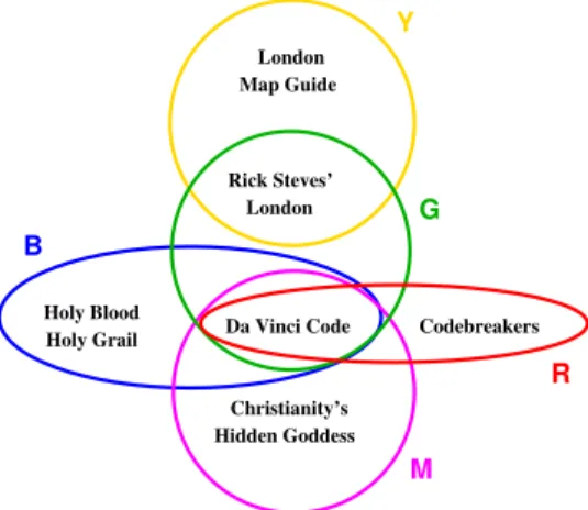
For instance, consider the set system in Fig. 1 where the six objects are books and the descriptors denote books about traveling in London (Y), books containing information about places where popes are interred (G), popular books about the history of codes and ciphers (R), books about Mary Magdalene (M), and books about the ancient Priory of Sion (B). An example redescription for this dataset is: ‘books involving Priory of Sion as well as Mary Magdalene are the same as non-travel books describing where popes are interred,’ or B∩M ⇔ G−Y. This is an exact redescription and gives two different ways of defining the singleton set {‘The Da Vinci Code’}. The basic premise of redescription mining is that object sets that can indeed be defined in at least two ways are likely to exhibit concerted behavior and are, hence, interesting. This problem is non-trivial because we are given neither the object sets to be redescribed nor the set-theoretic constructions to be used in combining the given descriptors.
While traditional redescription mining is focused on finding object sets that are similar, storytelling aims to explicitly relate object sets that are disjoint (and hence, maximally dissimilar). Given a start and end descriptor, the goal here is to find a path from one to the other through a sequence of intermediaries, each
London Map Guide Christianity’s Hidden Goddess Rick Steves’ London Holy Blood
Holy Grail Da Vinci Code Codebreakers
Y
G
R
M B
Figure 1: An example input to storytelling.
of which is an approximate redescription of its neighbor(s). An example story in the above dataset results when we try to relate London travel books to books about codes and cipher history: Some London travel books (Y) overlap with books about places where popes are interred (G), some of which are books about ancient codes (R). This story is a sequence of (approximate) redescriptions: Y ⇔ G ⇔ R. Each step of this story holds with Jaccard’s coefficient 1/3 (the ratio of the size of common elements to elements on either side of the redescription). A stronger story, that holds with Jaccard’s coefficient 1/2 at each step, is:
B⇔(G∩M)⇔R.
Why is this problem interesting and relevant? Storytelling finds application in many domains, such as bioinformatics, computational linguistics, document modeling, social network analysis, and counter-terrorism. In these contexts, stories reveal multiple forms of insights. First, since intermediaries must conform toa priori knowledge, we can think of storytelling as a carefully argued process of removing and adding participants, not unlike a real story. Knowing exactly which objects must be displaced, and in what order, helps expose the mechanics of complex relationships. Second, storytelling can be viewed as an abstraction of relationship navigation for propositional vocabularies and offers insights similar to what we expect to gain from techniques such as inductive logic programming applied to multi-relational databases. Third, storytelling reveals insight into how the underlying Venn diagram of sets is organized, and how it can be harnessed for explaining disjoint connections. In particular, we can investigate if certain sets have greater propensity for participating in some stories more than others. Such insights have great explanatory power and help formulate hypotheses for situating new data in the context of well-understood processes. Finally, in domains such as bioinformatics, the emergence of high-throughput data acquisition systems (e.g., genome-wide functional screens, microarrays, RNAi assays) has made it easy for a domain scientist to define vocabularies and sets. We argue that these domains are now suffering from ‘descriptor overload’; storytelling promises to be a valuable tool to attack this problem and reconcile disparate vocabularies.
Why is this problem difficult? Storytelling is non-trivial because the space of possible descriptor expres-sions is not enumerable beforehand and hence the network of overlap relationships cannot be materialized statically. In a typical application, we have hundreds to thousands of objects and an order of magnitude greater descriptors, with an even larger number of possible set-theoretic constructions made of the descriptors. Effective storytelling solutions must multiplex the task of constructive induction of descriptor expressions with focused search toward the end point of the story.
The main contributions of this paper are the introduction of the storytelling problem, its formalization as a generalization of redescription mining, and an efficient storytelling implementation that embeds the CARTwheels redescription mining algorithm [14] in an A* search procedure. We also showcase three appli-cations of storytelling: a study of word overlaps in large English dictionaries, exploring connections between genesets in a bioinformatics dataset, and relating publications in the PubMed index of abstracts. All these applications reveal insight into the underlying vocabularies and present significant potential for knowledge discovery.
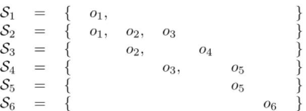
S1 = { o1, } S2 = { o1, o2, o3 } S3 = { o2, o4 } S4 = { o3, o5 } S5 = { o5 } S6 = { o6 }
Figure 2: Example data for illustrating operation of storytelling algorithm.
2
Background
The inputs to storytelling are the universal set of objectsO(e.g., books, genes) and a collectionS of subsets of O. The elements of S are referred to as the descriptors Si, and assumed to form a covering of O, i.e.,
S
iSi = O. In addition, two elements ofS are designated as the starting descriptor (X) and the ending descriptor (Y), where typically X ∩Y = φ. In the simplest version of storytelling, we must formulate a sequence of descriptors (called a story) Z1,Z2,· · ·,Zk ∈ S where Z1 = X, Zk = Y, and J(Zi, Zj) ≥θ, 1< i≤k, j=i+ 1, θ being a user supplied threshold. Here,J denotes the Jaccard’s coefficient between two sets, given by: J(Zi, Zj) = ||ZZi∩Zj|
i∪Zj|. J is zero if the sets are disjoint, is one if they are the same, and is between zero and one if either descriptor is a subset of the other, or when they are overlapping. Every successive pair of descriptors in the story constitutes a redescription, Zi ⇔ Zj, whose left and right sides (approximately) induce the same subset ofO. Observe that storytelling can progress only when redescriptions are strictly approximate, i.e., when 0<J(Zi, Zj)<1.
In the generalized version of storytelling studied here, the intermediariesZiare not constrained to be just elements ofS but can be set-theoretic expressions made up of theSi’s, e.g.,S1∪ S3,S2− S4,S1∩(S2∪ S5). In this case, to ensure well posedness, we will require that all participating expressions conform to a given bias, e.g., monotone forms, conjunctions, or are otherwise length-limited.
There are many algorithms proposed for mining redescriptions, some based on systematic enumeration and pruning (e.g., CHARM-L [18]) and some based on heuristic search (e.g., CARTwheels [14]). These algorithms also differ in their choice of bias (conjunctions in CHARM-L, and depth-limited DNF expressions in CARTwheels). We focus on CARTwheels as it provides the exploratory features necessary to incrementally construct stories.
CARTwheels exploits the fact that redescriptions never occur in isolation but rather in pairs or other groups. For instance, redescription Zi ⇔ Zj coexists with ¬Zi ⇔ ¬Zj. This property is used to search for matching partitions (here, {Zi,¬Zi} and{Zj,¬Zj}) by growing two binary decision trees (CARTs) in opposite directions so that they are matched at the leaves. The nodes in these trees correspond to boolean membership variables of the given descriptors so that we can interpret paths to represent set intersections, differences, or complements; unions of paths would correspond to disjunctions. Essentially, one tree exposes a partition of objects via its choice of descriptors (e.g., Zi) and the other tree tries to grow to match this partition using a different choice of descriptors (Zj). If partition correspondence is established, then paths that join define redescriptions. CARTwheels explores the space of possible tree matchings via an alternation process whereby trees are repeatedly re-grown to match the partitions exposed by the other tree.
Unlike previous work, where CARTwheels alternation was configured to enumeratively explore the space of all redescriptions [14], the main contribution of the present paper is to demonstrate how we can focus the alternation toward a target descriptor.
3
Designing a Storyteller
We embed CARTwheels inside an A* search procedure, using the former to supply next move operators on search branches to the latter. Each move is a possible redescription to be explored and a heuristic function evaluates these redescriptions for their potential to lead to the end descriptor of the story. In this paper,
obj. S2 S3 S4 S5 S6 class o1 √ × × × × S1 o2 √ √ × × × S1 o3 √ × √ × × S1 o4 × √ × × × S1 o5 × × √ √ × S1 o6 × × × × √ S1 obj. S1 S3 S4 S5 S6 class o1 √ × × × × (S2− S3) o2 × √ × × × (S2− S3) o3 × × √ × × (S2− S3) o4 × √ × × × (S2− S3) o5 × × √ √ × (S2− S3) o6 × × × × √ (S2− S3)
Figure 3: (left) Dataset to initialize storytelling algorithm. (right) Dataset for the second iteration. we focus on story length—number of redescriptions to reach the end descriptor—as the primary criterion of optimality although different criteria might be more suitable in other applications. Backtracking happens when a previously unexplored move (redescription) appears more attractive than the current descriptor. The search terminates when we reach a descriptor that is within the specified Jaccard’s threshold from the ending descriptor or when there are no redescriptions left to explore.
3.1
Working Example
For ease of illustration, consider the artificial example in Fig. 2 with six descriptors{S1,S2,S3,S4,S5,S6} defined over the universal setO={o1, o2, o3, o4, o5, o6}(in a realistic application, the number of descriptors would greatly exceed the number of objects). Our goal is to find a story between descriptorS1, corresponding to the set{o1}, andS5, corresponding to the set{o5}, such that each step is a redescription that holds with Jaccard’s coefficient at leastθ= 0.5. In this example, we set the maximum depth of decision trees used to 2.
To initialize the alternation, we prepare a traditional dataset for classification tree induction (see Fig. 3, left), where the entries correspond to the objects, the class (to be learnt) corresponds to the starting de-scriptor, and the boolean features are comprised of the remaining descriptors. A classification tree can now be grown using these features and class assignments, using the Jaccard’s coefficient as the node evaluation criterion. Hence, at each level in the decision tree we construct, we look for a descriptorSi such that one of the blocks in its induced partition will provide the best overlap with the class we seek (in this case,S1). If the maximum Jaccard’s coefficient value obtainable is lesser thanθ, we choose the descriptor that provides the best value. Else, we consider all descriptors that satisfy the Jaccard’s threshold and, among them, greedily choose the one with the highest Jaccard’s coefficient with the end point of the story. The tree growth is continued until the maximum Jaccard’s coefficient observed at a given depth is lesser than that observed at the parent level, or the depth limit of tree growth is reached. Once the tree has been constructed, class assignments at the leaves are made by majority and paths that lead to a given class are union-ed to form redescriptions.
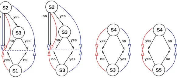
For instance, Fig. 4 (a) shows the decision tree we have constructed to match the partition{S1,S1}. This tree provides the first step in the story to be the redescriptionS1⇔(S2− S3). In this example, we show only one possible ‘next tree’ for our example but in our implementation, we maintain a number of such possible matching trees, to simulate a branching process and for potential backtracking. Note that while the current redescription holds with a Jaccard’s value of 0.5, the new descriptor does not have any overlap withS5.
For the next step in our story, we use the partition {(S2− S3),(S2− S3)} as the classes to match and consider the dataset as shown in Fig. 3 (right). In constructing the new dataset, observe that we ignore the descriptor that is the top-most node (here, S2) in the decision tree that defines the current partition. This ensures that we do not utilize the same features for matching a partition as those that define the partition! The one-level tree we learn at this stage is shown in Fig. 4 (b). The redescription of interest here is (S2− S3)⇔ S3, which also holds with a Jaccard’s coefficient of 0.5. Although it introduces the element we seek (o5), the redescription to the end point of the story,S3 ⇔ S5, has only a Jaccard’s coefficient of 0.25. We hence continue the search and obtain the redescriptionS3⇔ S4 which gives us the desired overlap with the target, and our final redescription, namelyS4⇔ S5. Our story is thusS1⇔(S2− S3)⇔ S3⇔ S4⇔ S5.
S1 yes no yes no yes no S2 S3 (a) S4 no yes S5 yes no (d) S4 no yes S3 no yes (c) S3 no yes yes no yes no S2 S3 (b)
Figure 4: Storytelling using CARTwheels alternation. Beginning with S1, the starting descriptor exposed by the bottom tree in (a), the alternation systematically moves towardS5, the ending descriptor in (d). At each step we alternately keep one of the trees fixed and grow a new tree to match it. The story mined here is the sequence of redescriptions: S1⇔(S2− S3)⇔ S3⇔ S4⇔ S5.
3.2
Implementation
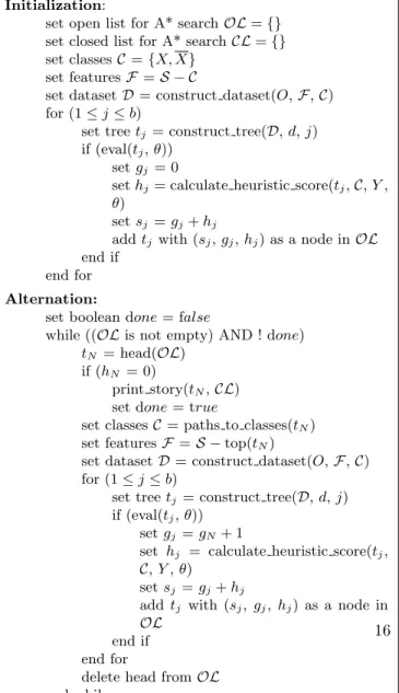
The storytelling algorithmic framework is shown in Table 1 and follows the outline of the working example above. The key utility functions are: construct dataset, that prepares the dataset D at each alternation;
construct tree, that is calledb (branching factor) times at each step to create trees of desired depth limitd;
eval, which determines if the Jaccard’s coefficient between the current descriptor and the union of the paths leading to it in the current tree have a Jaccard’s coefficient higher than or equal toθ;calculate heuristic score, which computes the heuristic score for each tree; andprint story, which prints the story by tracing back the sequence of mined redescriptions.
In the outer A* search procedure, qualified trees are placed in the open listOL (a priority queue) and considered in order of their evaluations. If the heuristic evaluation hN for the currently picked tree tN is zero, we have arrived at a tree that has sufficient Jaccard’s overlap with the end point of the story and we terminate. If hN is not zero, a new set of classes C for objects in O are induced using the function
paths to classes,tN is moved to the closed list, and all trees induced byconstruct treeare placed in the open list. This process is repeated until there is no tree left in the open list or a story has been found.
Just as the notion of ‘class’ is revised periodically at each alternation, so are the candidate set of ‘features.’ Observe that, in the Initialization step, the set of possible features involves all except the starting descriptor. Inside the Alternation subroutine, the candidate set of features is made equal to all except the feature used at the root of the current tree (supplied by the routinetop).
The heuristic scorehj for tree tj is combined with cost expended so far (gj) to arrive at the evaluation criterionsj. Nodes inOLare hence ordered bysj. We assume unit cost per redescription so that the story length is the number of redescriptions required to traverse to the ending descriptor. The heuristic function
h is designed to systematically never over-estimate the number of redescriptions remaining and takes the value of zero for a tree whose partition is within the specified Jaccard’s coefficient to the ending descriptor. We now present details ofhand prove its admissibility.
Table 2 outlines the approach to estimate hj for tree tj. This algorithm can be understood as follows. Assume that the new descriptorZj(provided by treetj) hasf elements in common with the target descriptor
Y andeelements that do not participate inY. This means thatZj must shed enough of theeelements and acquire enough of the|Y| −f elements in order to have a Jaccard’s threshold of ≥θ withY. The goal of
calculate heuristic score is to estimate the number of redescriptions required to shed the requisite number among eelements and acquire some of the necessary |Y| −f elements. The procedure first conservatively estimates if the current discrepancies already correspond to a Jaccard’s threshold of≥θ with Y, in which case it returns zero. If this is not possible, the procedure estimates the shortest number of steps in which the deletions and additions can happen by a recursive computation. Two extremes are considered at each step – the case where we can acquire as many of the necessary new elements as dictated byθ without any removals, and the case where we can shed as many of the unnecessary elements as dictated byθwithout any additions. This step provides us the bounds δfmax and δemax in Table 2. We then search combinatorially within these ranges for the maximal number of deletions, for every possible number of additions, such that
θholds, akin to dynamic programming. The minimum number of redescriptions over all possibilities is then returned. It is easy to see that
Lemma 1 The heuristic defined by calculate heuristic score is admissible.
3.3
Data structures
The efficient implementation of our storytelling algorithm hinges on data structures for fast estimation of overlaps. This problem has been studied by the database community in various guises, e.g., similarity search [11] and set joins on similarity predicates [15]. Specific solutions advocate the use of signature trees [7], hierarchical bitmap indices [10], and locality sensitive hashing [4], especially the technique of min-wise independent permutations [2] that is particularly geared toward the Jaccard’s coefficient. In this paper, we combine an AD-tree data structure [9] with the signature tables [1] approach for efficient similarity search in categorical data.
The signature table is constructed before the Initialization step mentioned in Table 1. Here, objects in the universal set are divided into a predefined number of clusters (c) on the basis of their co-occurrence frequencies. This is achieved by first constructing a graph where each object is a node and objects that co-occur form edges. Each edge is associated with a weight which is the inverse of the co-co-occurrence frequency for that edge. The weight associated with each node is the sum of the weights of each edge it is a part of. The total weight of the graph is the sum of the weight of all nodes. We set the critical weight of the graph to be the total weight divided byc. For finding each cluster, we begin with the nodes that are a part of the edge that currently has the minimum weight associated with it. We delete these nodes from the graph and add them to the current cluster. The weight of the cluster is now the sum of the weights of nodes it contains (as obtained from the original graph). We continue to add nodes to the cluster that have the minimum weight in an edge associated with any of the objects that already are a part of the cluster. This continues till the weight of the cluster is greater than the critical weight. At this point, we recalculate the critical weight on the basis of the nodes remaining in the original graph and proceed to finding the next set of nodes, till allc
clusters have been found.
Each descriptor, originally a binary vector size |O|, can now be condensed into a binary vector (the signature) of sizecby encoding a 1 for each cluster that has an object present in the descriptor and a 0 for each cluster that has no object in the descriptor.
All descriptors and their co-occurrence frequencies (used in constructing a decision tree of depth more than 1) are also built into an AD-tree at this stage. The descriptors at the top-level of the AD-tree are additionally linked to their signatures. When a similarity search query is issued, only nodes that correspond to signatures of interest need to be investigated. At greater depths in the AD-tree, we can either construct individual signature tables for each node in the AD-tree or we can opt to use a traditional AD-tree node that contain descriptor names and co-occurrence frequencies. In our implementation, we used traditional AD-tree nodes at depth greater than 1.
Using these data structures, we can reduce the number of descriptors searched against at each step and improve the speed of computation of stories. For instance, in the first call to the function construct tree, where we are looking for the best match for the classX from among the descriptor setD, we can reduceX
YGL158W YJL164C YKL035W kinase hexokinase protein modification YCL040W YFR053C YGL158W YJL164C YKL035W YCL040W YDR516C YFR053C YGL158W YGR052W YJL164C YCL040W YDR516C YFR053C cell growth and/or maintenance transferase, transferring P-containing groups
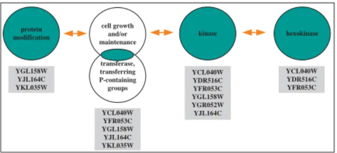
Figure 5: A significant story among gene sets from protein modification to hexokinase.
clusters in the form of a frequency vectorfc. The optimistic Jaccard’s coefficient (OJ) betweenXc and a signature vectorVc
i corresponding to a set of descriptors can then be calculated by the formula
OJ(Xc, Vic) = Pc j=1(f c[j]∗Xc[j]∗Vc i[j]) Pc j=1fc[j]
We then compare Xc to all the signature vectors and retain only those for which the optimistic Jaccard’s coefficient is aboveθ. This narrows down our search to only those descriptors that have potential to provide the necessary overlap.
3.4
Assessing Significance of Stories
The significance of a story is assessed at the level of each redescription participating in the story. To assess the significance of redescriptionX ⇔Y, we use the cumulative hypergeometric distribution to determine the probability of obtaining a rate of co-occurrence ofX andY (over the object domain), given their marginal occurrence probabilities, and comparing it to the observed rate of co-occurrence by chance. To account for multiple hypothesis testing, the significance threshold is determined by first characterizing the distribution for all descriptors tested and determining if the given redescription has a rate of occurrence more than four standard deviations above the mean.
4
Experimental Results
Our three experimental studies are meant to illustrate different aspects of our storytelling algorithm and implementation. The first study characterizes word overlaps in large English dictionaries and illustrates scalability of the implementation and how the different parameter settings affect the quality of stories mined. The second study, involving gene sets in bioinformatics, showcases the constructive induction capabilities of CARTwheels when used for storytelling. This study and the third, which builds stories between PubMed abstracts, also illustrate interesting nuggets of discovered knowledge.
4.1
Word Overlaps
In our first study, we implement storytelling for the MorphWord puzzle wherein we are given two words, e.g., PURE and WOOL, and we must morph one into the other by changing only one letter at a time
(meaningfully). One solution is: PURE → PORE →POLE → POLL → POOL →WOOL. Here we can
think of a word as a set of (letter, position) tuples so that all meaningful English words constitute the descriptors. Each step of this story is an approximate redescription between two four-element sets, having three elements in common. It is important to note that words that are anagrams of each other (e.g., ‘ELVIS’ and ‘LIVES’) willnothave a Jaccard’s coefficient of 1, since position is important.
We harvested words of length 3 to 13 words from the Wordox dictionary of English words (http://www. esclub.gr/games/wordox/), yielding more than 160,000 words. Consistent with the MorphWord puzzle, we
Early expression of yeast genes affected by chemical stress (PMID:15713640; 2005–02–16)
⇓
Glutathione, but not transcription factor Yap1, is required for carbon source-dependent
resistance to oxidative stress in
Saccharomyces cerevisiae
(PMID:10794174; 2000–06–22)
⇓
The role of glutathione in yeast dehydration tolerance (PMID:14697735; 2003–12–30)
⇓
The adaptive response of
Saccharomyces cerevisiae
to mercury exposure (PMID:11816031; 2002–01–29)
⇓
Cloning, characterization, and expression of the CIP2 gene induced under cadmium stress inCandida sp.
(PMID:9627968; 1998–07–09)
⇓
Mutations in the Schizosaccharomyces pombe
heat shock factor that differentially affect responses to heat and cadmium stress
(PMID:10071222; 1999–04–07)
⇓
Genome-wide analysis of the biology of stress responses through heat shock transcription factor
(PMID:15169889; 2004–05–31)
⇓
Isolation and characterization of HsfA3, a new heat stress transcription
factor ofLycopersicon peruvianum
(PMID:10849352; 2000–10–10)
⇓
Heat stress transcription factors from tomato can functionally replace HSF1 in the yeastSaccharomyces cerevisiae
(PMID:9268023; 1997-09-18)
restrict all CARTs to be of depthd= 1 and study the effect of θ andb on the number of stories possible, length of stories mined, and time taken to mine stories. For ease of interpretation, we recast Jaccard’s thresholds in terms of the number of letters in common (lc) between two words. Although MorphWord is traditionally formulated withlc= 1, we explore higherlcvalues as well. Due to space restrictions, we present our results on subsets of the master word list, namely 5 letter words (L5) and 10 letter words (L10). In each case, we selected 100,000 pairs of words at random and tried to find stories between them, with different
lc and b settings. An example story we mined with five letter words (with setting lc= 3) is: BOOTH ⇔
BOATS⇔BEAMS⇔DEADS⇔GRADS⇔GRADE⇔CRAZE⇔CRASH⇔FLASH.
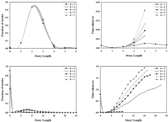
Fig. 7 (first column) depicts plots of the fraction of stories (out of 100,000) mined with various story lengths as a function oflc, for a branching factorb= 5. In these plots, a story length of 0, rather counter-intuitively, implies that no story was found for the word pair considered. The critical story length where the majority of stories are mined steadily increases aslc is increased. This is because, as lcis increased, more overlap is required at each step of the story such that it takes longer for one word to morph into another. At the same time, the total number of stories mined decreases aslc is increased, due to the lack of viable redescriptions.
To study the effect ofbon the length of stories mined, we focus our attention onlcvalues of 2 forL5and 5 forL10. Fig. 8 (first column) shows plots of the fraction of stories mined with various lengths as a function ofb. As before, a path length of 0 in the plots implies that no story was found for the word pair considered. Here, there are qualitative changes between the two datasets (Fig. 8, first column, top and bottom rows).
For L5, the lc value chosen (2) supports a significant number of short stories. This lc value affords a high number of possible redescriptions per descriptor (about 20–100), making it highly likely that the A* algorithm will follow a path that leads close to the target word. In other words,bdoes not have as significant an impact for this dataset.
ForL10, thelcvalue chosen contributes to a higher probability of longer stories. As a result the branching factor b plays a crucial role. This is evident in the case ofb = 1, where the excessively greedy strategy is often rendered futile. Asb increases, the chances of going down toward the target word increases and more stories are mined.
To study the effect of these parameters on the time required to mine stories, we set b= 5 as before for understanding the role oflc. We computed the average time taken to mine a story, for various story lengths, across all pairs of words considered. Fig. 7 (second column) shows plots of this average time against story lengths, for different lc values. Again, the general behavior in the two graphs is quite similar. There is a near linear increase in time required, with steeper increases for lowerlcvalues. This is because the lowerlc
values cause an increase in the number of possibilities (within the bound of b= 5) which must be explored before converging on the shortest path. Also observe the higher times for story lengths of 0, indicating it takes longer to conclude that stories do not exist. Similar linear trends are observed in time versus the role of b (Fig. 8, second column). Here, steeper profiles are witnessed for higher b values. Once again, this is due to the increase in the number of possibilities, although as Fig. 8, second column (bottom panel) shows, these increases appears to taper off quickly.
These figures clearly indicate the underlying tradeoff in mining stories: time versus importance of optimal story lengths.
4.2
Gene Sets
In our second case study, we mine stories among descriptors defined over gene sets in the budding yeastS. cerevisiae. We draw our descriptors from various bioinformatics vocabularies (e.g., the Gene Ontology (GO), microarray experiment clusters, experiment ranges) as done in previous work [14, 18]. An example significant story, between the GO categories protein modification and hexokinase, mined forθ= 0.5,b= 5, andd= 2 is shown in Fig. 5. Observe that the second descriptor in the story involves a set intersection performed by CARTwheels. A unifying feature that links the genes in this story is their common role in nutrient control and carbohydrate metabolism, particularly metabolism of glucose-phosphate. Considering the three genes in the first descriptor, YKL035W is involved in the reversible conversion of glucose-1-phosphate to UDP-glucose via UTP; YJL164C is a cAMP dependent kinase and binds both YFL033C (glucose repressed, nutrient
Figure 7: (First column) Fraction of stories mined as a function of story length, for different values of lc. (Second column) Average time required to mine stories as a function of story length, for different values of
Figure 8: (First column) Fraction of stories mined as a function of story length, for different values of b. (Second column) Average time required to mine stories as a function of story length, for different values of
YBR247C YCL054W YPR112C -1 40 minutes -2 -3 -4 -5 -6 0 YBR247C YCL054W YPR112C -1 20 minutes -2 -3 -4 -5 -6 0 YBR247C YCL054W -1 10 minutes -2 -3 -4 -5 -6 0 nucleolus transcription from Pol I promoter YBR247C YCL054W -1 05 minutes -2 -3 -4 -5 -6 0 YBR247C YCL054W -1 15 minutes -2 -3 -4 -5 -6 0 -7 YBR247C YCL054W -1 30 minutes-5-4-3-2 -6 0 -7
Figure 9: Some descriptor expressions serve as the fulcrum point for many stories.
control) and YIL033C (glycogen accumulation); and YGL158W is a kinase that binds YGL115W (release from glucose repression). Two new genes enter the story with the first redescription, namely YCL040W (involved in phosphorylation of glucose) and YFR053C (a hexokinase also involved in the phosphorylation of glucose in the glycolysis pathway). In traversing the second redescription, two additional genes appear: YDR516C is involved in phosphorylation of glucose and, most importantly, also binds YCL040W (which is present in earlier redescriptions). YGR052W is a mitochondrial serine/threonine kinase of unknown function. Through the thread of the story we predict that YGR052W may also be involved in an aspect of glucose metabolism and/or nutrient control.
As a second example, we attempted to evaluate the propensity for certain descriptors to participate in more stories than others. For settings of θ = 0.1, b = 1, and d = 2, we mined significant stories between descriptors from one vocabulary to every other descriptor in the same vocabulary, through a different vocabulary. These story chains were then analyzed to find frequently occurring descriptors. One example of a pattern we found is shown in Fig. 9 where an intersection of two GO descriptors serves as the central node in a variety of stories, each of length two. Note that set constructions happen at the end points of the story as well, giving us bucketed ranges over gene expression values. For instance, the leftmost expression in Fig. 9 denotes the conjunction ‘expression≤ −1.5 AND NOT (expression≤ −3).’ The products of the three participating genes all involve some aspect of the processing of ribosomal RNA and therefore have critical functions. YBR247C and YCL054W proteins have many documented interactions and the majority of these are with rRNA processing proteins. YPR112C has no documented interactions. These three genes may be viewed as perhaps having key regulatory roles during the response of the cells to heat shock. Following initial exposure to stress they are rapidly down-regulated and remain so until 30 to 40 minutes. The alleviation of down regulation after this time may reflect an adaptive response of the cells to the heat shock via de novo protein synthesis.
4.3
PubMed Abstracts
For our final case study, we consider the more than 140,000 publications about yeast in the PubMed in-dex and focus on finding stories between publication abstracts. Each abstract is hence a descriptor over terms/keywords. We restrict our CARTs to be of depth 1 and also adopt a weighted Jaccard’s measure that is more suited to measuring similarity between bags (details omitted due to space constraints). To generate keywords, we focused on the 3756 abstracts containing the keywords ‘yeast AND stress’ and applied stop word removal and Porter’s stemming as well as manual inspection to cluster similar words together. Over 95% of the keywords were eliminated by significance testing over the values ofT F ·IDF (corresponds to a threshold of about 7), resulting in 6821 unique words.
For this application, it is important to note that the computation of the heuristic function would result in a combinatorial problem since each word does not uniformly have a weight of 1 in our Jaccard’s calculation.
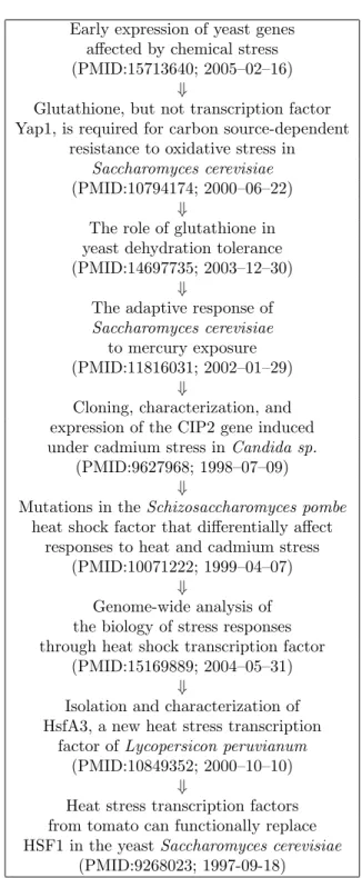
For instance, elimination of different word subsets from a given descriptor, even if they are of the same size, will result in different Jaccard’s coefficients; hence we will have to exhaustively search all combinations for removal and addition of keywords to determine the theoretically shortest possible storylength. Thus, for the case of the weighted Jaccard’s coefficient, we used a simpler heuristic function wherein we estimate the maximum weight we can gain/lose at each step and calculated the number of steps required to gain enough of the weight for the final document and lose enough weight from the current document, to reach a Jaccard’s coefficient above the threshold for the final document. Two examples of significant stories we mined using this function are given in Figs 6 and 10 (the PubMed IDs and publication dates are given alongside).
The first story (see Fig. 6), mined withθ= 0.2, b= 5, begins with a high throughput experiment that links chemical stress to gene expression inSaccharomyces cerevisiae, and ends with heat stress transcription factors in tomato. The ‘story line’ was initiated through comparisons between oxidative and heavy metal stresses. This led to a paper identifying a gene fromCandida sp. that was expressed when the cells are exposed to cadmium but not copper, mercury, lead or manganese. Interestingly a BLAST search for the encoded protein sequence indicates that the protein is novel. The link between tomato heat stress transcription factors and a cadmium-specific gene with no known match in the current databases was through work with the fission yeast Schizosaccharomyces pombewhere a study looked specifically at heat and cadmium stress responses. This story hence illustrates the key players in the systems biology of related chemical stresses.
For our next example, we mined for stories that follow a strict sequential order of publication year. One example here is shown in Fig. 10, with settingsθ= 0.4, b= 5. The featured compound in this story—cAMP (cyclic adenosine monophosphate)—is a signaling molecule found in all forms of life. In yeast it serves as a relay for glucose levels, effecting distinct responses in accord with nutrient need and availability. This ‘backwards in time’ story starts with a paper that addresses specific changes in gene transcription modulated by cAMP levels inSchizosaccharomyces cerevisiae. It was connected with a paper that also addressed the relationship between nutrients and cAMP, but with a different yeast (Saccharomyces cerevisiae) and with a different emphasis (partners upstream and downstream of where cAMP intersects the pathway). The third paper in the story describes the relationship between a serine/threonine protein kinase (Snf1) and nutrient levels, and how it is related to AMP concentrations (the degradation product of cAMP), while the fourth paper links catalase gene expression to cAMP. Together these four papers provide a continual story line on how yeast responds to changes in nutrient levels. Interestingly, Paper #4 has been cited 82 times (as of March 2006), Paper #3 114 times, and Paper #2 182 times (Paper #1 is too new to be heavily cited). However, the only connection between them in the citation indices is that Paper #2 has referenced paper #4.
5
Related Research
We briefly survey related research in three categories: storytelling in information visualization, approaches for topic tracking in documents, and link mining.
In the first category, storytelling has been viewed, not in a data mining context, but as an information organization tool based on narrative structures from real life. Kuchinsky et al. [6] propose an interactive approach for biological information management using three constructs – items, collections (of items), and stories. A ‘story editor’ is used to form an outline of the story using a template. The players (items and itemsets) are then used to fill in the template manually to complete the story.
Pertinent work in the topic tracking community, e.g., [5] focuses on post-processing search results into storylines by analyzing bipartite graphs of document-term relationships. Here a story is a thread of related documents with temporal as well as semantic coherence. Although similar to our PubMed abstracts case study, these works are focused on unsupervised discovery of all threads whereas we focus on directed storylines between given start and end points. Furthermore, as shown in our GeneSets case study, we allow arbitrary set constructions for the purpose of positing overlaps by casting stories as a generalization of redescriptions. The definition of a ‘thread’ is also different in this work and relies on the notion of node-disjoint directed paths.
Suppressors of an adenylate cyclase deletion in the fission yeast
Schizosaccharomyces pombe
(PMID:15189983; 2004–06–10)
⇓
Novel sensing mechanisms and targets for the cAMP-protein kinase A pathway in
Saccharomyces cerevisiae
(PMID:10476026; 1999–10–21)
⇓
Deletion of SNF1 affects the nutrient response of yeast and resembles mutations which activate
the adenylate cyclase pathway (PMID:1752415; 1992–01–24)
⇓
Negative regulation of transcription of theSaccharomyces cerevisiae catalase T (CTT1) gene by cAMP is mediated by
a positive control element (PMID:1848176; 1991–04–15)
Figure 10: An example significant story among PubMed abstracts around cAMP levels.
can be approached as a problem of analyzing overlap relationships. However, the links used and sought by us are between sets of items rather than individual items, and these sets are not enumerated beforehand. The concept of stories is also inherently similar in spirit to relational knowledge discovery, e.g., [12], but observe that our vocabularies are primarily propositional in nature, and defined over a single domain of objects. In future work, we aim to generalize story telling into relational redescription mining where the stories can straddle different domains and employ relationships for navigating across domains.
Finally, the applications presented here suggest comparisons to classical discovery systems such as Swan-son’s Arrowsmith [17] which can be viewed as seeking stories of length two. Our stories can be of arbitrary lengths with differing complexities of the participating descriptors.
6
Discussion
By defining stories as chains of redescriptions, we have been able to design a storytelling algorithm as A* search around the outputs of a redescription mining algorithm. We have demonstrated the scalability of this approach using the Word overlaps case study and showcased its potential for knowledge discovery using the Gene sets and PubMed abstracts case studies.
In future work, we aim to investigate other metrics for evaluating stories besides story length, e.g., based on the number of objects temporarily brought into the story, the story’s conformance to prior background knowledge, or using overlap metrics that better mirror a domain scientist’s conception of set similarity. We also aim to explore connections to works that characterize the structure of partitions [8, 16] and investigate whether storylines can be designed around paths in such discrete structures. We also intend to generalize from propositional to predicate vocabularies and cast storytelling in the context of relational redescriptions. This will help provide structured stories that follow a template of connections. Our eventual goal is to establish storytelling as an important tool for reasoning with data and domain theories.
References
[1] C.C. Aggarwal, J.L. Wolf, and P.S. Yu. A New Method for Similarity Indexing of Market Basket Data. InProc. SIGMOD’99, pages 407–418, 1999.
[2] A.Z. Broder, M. Charikar, A.M. Frieze, and M. Mitzenmacher. Min-Wise Independent Permutations.
JCSS, Vol. 60(3):pages 630–659, June 2000.
[3] L. Getoor. Link Mining: A New Data Mining Challenge. SIGKDD Explorations, Vol. 5(1):pages 84–89, 2003.
[4] A. Gionis, P. Indyk, and R. Motwani. Similarity Search in High Dimensions via Hashing. In Proc. VLDB’99, pages 518–529, Sep 1999.
[5] R. Guha, R. Kumar, D. Sivakumar, and R. Sundaram. Unweaving a Web of Documents. In Proc. KDD’05, pages 574–579, 2005.
[6] A. Kuchinsky, K. Graham, D. Moh, A. Adler, K. Babaria, and M.L. Creech. Biological Storytelling: a Software Tool for Biological Information Organization based upon Narrative Structure. ACM SIG-GROUP Bulletin, Vol. 23(2):pages 4–5, Aug 2002.
[7] N. Mamoulis, D.W. Cheung, and W. Lian. Similarity Search in Sets and Categorical Data using the Signature Tree. InProc. ICDE’03, pages 75–86, 2003.
[8] M. Meila. Comparing Clusterings by the Variation of Information. In Proc. COLT’03, pages 173–187, 2003.
[9] A.W. Moore and M.S. Lee. Cached Sufficient Statistics for Efficient Machine Learning with Large Datasets. JAIR, Vol. 8:pages 67–91, 1998.
[10] M. Morzy, T. Morzy, A. Nanopoulos, and Y. Manolopoulos. Hierarchical Bitmap Index: An Efficient and Scalable Indexing Technique for Set-Valued Data. InProc. ADBIS’03, pages 236–252, Sep 2003. [11] A. Nanopoulos and Y. Manolopoulos. Efficient Similarity Search for Market Basket Data. VLDB
Journal, Vol. 11(2):pages 138–152, 2002.
[12] J. Neville and D. Jensen. Supporting Relational Knowledge Discovery: Lessons in Architecture and Algorithm Design. InProc. Data Mining Lessons Learned Workshop, ICML’02, 2002.
[13] L. Parida and N. Ramakrishnan. Redescription Mining: Structure Theory and Algorithms. In Proc. AAAI’05, pages 837–844, 2005.
[14] N. Ramakrishnan, D. Kumar, B. Mishra, M. Potts, and R.F. Helm. Turning CARTwheels: An Alter-nating Algorithm for Mining Redescriptions. InProc. KDD’04, pages 266–275, 2004.
[15] S. Sarawagi and A. Kirpal. Efficient Set Joins on Similarity Predicates. InProc. SIGMOD’04, pages 743–754, June 2004.
[16] D.A. Simovici and S. Jaroszewicz. An Axiomatization of Partition Entropy. IEEE Transactions on Information Theory, Vol. 48(7):pages 2138–2142, 2002.
[17] D.R. Swanson and N.R. Smalheiser. An Interactive System for Finding Complementary Literatures: A Stimulus to Scientific Discovery. Artificial Intelligence, Vol. 91(2):pages 183–203, 1997.
[18] M.J. Zaki and N. Ramakrishnan. Reasoning about Sets using Redescription Mining. InProc. KDD’05, pages 364–373, 2005.
Table 1: Storytelling algorithmic framework.
Input:
1. a domain of objectsO;
2. a collectionS of sets defined overO;
3. a designated starting descriptorX∈ S; and
4. a designated ending descriptorY ∈ S.
Parameters:
1. a threshold θ (0 < θ < 1) denoting the minimum
required Jaccard’s coefficient for each connection in the story;
2. d (depth of trees) that imposes a bias B over set
expressions defined onS; and
3. branching factorbthat restricts the maximum
num-ber of possible next states from each state in the A* search.
Output: a story comprising a sequence of
interme-diaries Z1, Z2,· · ·, Zk, such that X = Z1, Y = Zk,
J(Zi, Zi−1) ≥ θ,1 < i ≤ k, and each of Zi’s is in the desired biasB.
Initialization:
set open list for A* searchOL={}
set closed list for A* searchCL={}
set classesC ={X, X}
set featuresF =S − C
set datasetD= construct dataset(O,F,C) for (1≤j≤b)
set treetj= construct tree(D,d,j) if (eval(tj,θ))
setgj = 0
sethj= calculate heuristic score(tj,C,Y,
θ)
setsj =gj+hj
addtj with (sj,gj,hj) as a node inOL
end if end for
Alternation:
set boolean done= false
while ((OLis not empty) AND ! done)
tN = head(OL)
if (hN = 0)
print story(tN,CL) set done= true
set classesC = paths to classes(tN) set featuresF =S −top(tN)
set datasetD= construct dataset(O,F,C) for (1≤j≤b)
set treetj= construct tree(D,d,j) if (eval(tj,θ))
setgj=gN+ 1
set hj = calculate heuristic score(tj,
C,Y,θ) setsj=gj+hj
add tj with (sj, gj, hj) as a node in
OL
end if end for
Table 2: Heuristic for storytelling A* search.
calculate heuristic score(tj, C, Y, θ):
setZj−i = target class fromC
setZj = block fromtj that redescribes toZj−1
setf =|Zj∩Y| sete=|Zj−Y| seth= 0 calculateh= minpath(f,e,|Y|,h,θ) returnh minpath(f,e,|Y|, h, θ): calculateθY =f /(e+|Y|) if (θY ≥θ) returnh else
calculateδfmax =b(1−θ)(f+e)θ c
calculateδemax=b(1−θ)(f+e)c
sethmin=∞
for (i= 0;i≤δfmax;i=i+ 1)
setdone= false
for (k = δemax; k ≥ 0 and ! done; k =
k−1)
calculateθnew = f+e−kf+e+i if (θnew≥θ)
setdone= true
set hcurr = minpath(f+i, e−k,
|Y|,h+ 1,θ) if (hcurr < hmin)
sethmin=hcurr
end if end if end for end for returnhmin end if