Visual Navigation for Robots in Urban and Indoor Environments

VISUAL NAVIGATION FOR ROBOTS IN URBAN AND INDOOR ENVIRONMENTS

A Dissertation by YAN LU

Submitted to the Office of Graduate and Professional Studies of Texas A&M University

in partial fulfillment of the requirements for the degree of DOCTOR OF PHILOSOPHY

Chair of Committee, Dezhen Song

Committee Members, Ricardo Gutierrez-Osuna Dylan Shell

Wei Yan Head of Department, Dilma Da Silva

August 2015

Major Subject: Computer Engineering

ABSTRACT

As a fundamental capability for mobile robots, navigation involves multiple tasks in-cluding localization, mapping, motion planning, and obstacle avoidance. In unknown environments, a robot has to construct a map of the environment while simultaneously keeping track of its own location within the map. This is known as simultaneous local-ization and mapping (SLAM). For urban and indoor environments, SLAM is especially important since GPS signals are often unavailable. Visual SLAM uses cameras as the primary sensor and is a highly attractive but challenging research topic. The major chal-lenge lies in the robustness to lighting variation and uneven feature distribution. Another challenge is to build semantic maps composed of high-level landmarks. To meet these challenges, we investigate feature fusion approaches for visual SLAM. The basic ratio-nale is that since urban and indoor environments contain various feature types such points and lines, in combination these features should improve the robustness, and meanwhile, high-level landmarks can be defined as or derived from these combinations.

We design a novel data structure, multilayer feature graph (MFG), to organize five types of features and their inner geometric relationships. Building upon a two view-based MFG prototype, we extend the application of MFG to image sequence-based mapping by using EKF. We model and analyze how errors are generated and propagated through the construction of a two view-based MFG. This enables us to treat each MFG as an observation in the EKF update step. We apply the MFG-EKF method to a building exterior mapping task and demonstrate its efficacy.

Two view based MFG requires sufficient baseline to be successfully constructed, which is not always feasible. Therefore, we further devise a multiple view based algorithm to

construct MFG as a global map. Our proposed algorithm takes a video stream as input, initializes and iteratively updates MFG based on extracted key frames; it also refines robot localization and MFG landmarks using local bundle adjustment. We show the advantage of our method by comparing it with state-of-the-art methods on multiple indoor and outdoor datasets.

To avoid the scale ambiguity in monocular vision, we investigate the application of RGB-D for SLAM. We propose an algorithm by fusing point and line features. We extract 3D points and lines from RGB-D data, analyze their measurement uncertainties, and com-pute camera motion using maximum likelihood estimation. We validate our method using both uncertainty analysis and physical experiments, where it outperforms the counterparts under both constant and varying lighting conditions.

Besides visual SLAM, we also study specular object avoidance, which is a great chal-lenge for range sensors. We propose a vision-based algorithm to detect planar mirrors. We derive geometric constraints for corresponding real-virtual features across images and employ RANSAC to develop a robust detection algorithm. Our algorithm achieves a de-tection accuracy of 91.0%.

ACKNOWLEDGEMENTS

I would like to thank everyone who has helped me throughout my PhD study at A&M. The first one I want to thank is my advisor, Dr. Song, for his guide and support in the past five years. He brought me to robotics research, and gradually broadened my perspective over the field. He teaches me what is high quality research and how to do it. He is always willing to spend time with me discussing research plans, ideas, approaches, writing, etc. Especially, his patience in revising my paper drafts iteration by iteration greatly improved my technical writing. Dr. Song helped me not only in research, but also in many other aspects such as life and career planning. He has set up a good model for me to learn, and I will always be grateful to him.

I sincerely thank Drs. Haifeng Li, Jingtai Liu, Yiliang Xu, and Jingang Yi for being my great research collaborators and friends. My thank also goes to my friendly and supportive lab mates/alumni Chang-Young Kim, Wen Li, Ji Zhang, Matthew Hielsberg, Joseph Lee, Chieh Chou, Hsin-min Cheng, Xinran Wang, Madison Treat, and Rui Liu.

Last but not least, I would like to thank my advisory committee members Drs. Ricardo Gutierrez-Osuna, Dylan Shell and Wei Yan for their valuable time, insightful suggestions, and inspiring discussions.

TABLE OF CONTENTS Page ABSTRACT . . . ii DEDICATION . . . iv ACKNOWLEDGEMENTS . . . v TABLE OF CONTENTS . . . vi LIST OF FIGURES . . . ix

LIST OF TABLES . . . xii

1. INTRODUCTION . . . 1

2. LITERATURE REVIEW . . . 6

3. AUTOMATIC BUILDING EXTERIOR MAPPING USING MULTILAYER FEA-TURE GRAPH AND EXTENDED KALMAN FILTER* . . . 9

3.1 Related Work . . . 10

3.2 Problem Definition . . . 12

3.3 Observation Error: Uncertainty in MFG . . . 13

3.3.1 Error Modeling of Raw Features . . . 14

3.3.2 Error Analysis of Ideal Lines . . . 16

3.3.3 Error Analysis of Primary Planes . . . 18

3.4 EKF based Mapping with MFG . . . 21

3.4.1 System State Representation . . . 21

3.4.2 EKF Formulation . . . 22

3.4.3 Landmark Initialization and Management . . . 23

3.5 Experiments . . . 24

3.5.1 Uncertainty Test . . . 24

3.5.2 Field Mapping Test . . . 24

3.6 Conclusions . . . 27

4. VISUAL NAVIGATION USING HETEROGENEOUS LANDMARKS AND UNSUPERVISED GEOMETRIC CONSTRAINTS* . . . 28

4.1 Related Work . . . 29

4.2 Problem Formulation . . . 31

4.2.1 Assumptions and Notations . . . 31

4.2.2 Multilayer Feature Graph . . . 32

4.2.3 Problem Definition . . . 35

4.3 System Design and Multilayer Feature Graph . . . 35

4.3.1 Key Frame Selection . . . 35

4.3.2 2D MFG Construction and Matching . . . 37

4.3.3 Camera Pose Estimation . . . 41

4.3.4 3D MFG Update . . . 43

4.4 LBA and Pruning . . . 47

4.4.1 LBA with Geometric Constraints . . . 47

4.4.2 MFG Pruning . . . 50

4.5 Algorithms . . . 52

4.6 Experiments . . . 53

4.6.1 Line Matching Test . . . 53

4.6.2 Visual Odometry Test . . . 54

4.6.3 Test on KITTI Odometry Dataset . . . 63

4.7 Conclusions . . . 64

5. ROBUST RGB-D ODOMETRY USING POINT AND LINE FEATURES . . . 67

5.1 Related Work . . . 68

5.2 Problem Description and System Overview . . . 70

5.3 Feature Detection & Uncertainty Analysis . . . 71

5.3.1 Point Detection & Uncertainty Analysis . . . 71

5.3.2 Line Detection & Uncertainty Analysis . . . 72

5.4 Motion Estimation & Uncertainty Analysis . . . 76

5.4.1 Putative Feature Matching and RANSAC-based Motion Estimation 76 5.4.2 MLE of Motion and Uncertainty Analysis . . . 77

5.5 Experiments . . . 86

5.5.1 Test Under Varying Lighting . . . 86

5.5.2 Test on TUM Dataset Under Constant Lighting . . . 87

5.6 Conclusions . . . 89

6. ROBUST RECOGNITION OF MIRRORED PLANES USING TWO VIEWS* 91 6.1 Related Work . . . 92

6.2 Problem Definition . . . 93

6.3 Modeling . . . 95

6.4 Algorithm . . . 99

6.4.1 Quadruple Extraction . . . 99

6.4.2 Maximum Likelihood Estimation . . . 102 vii

6.4.3 Applying RANSAC Framework . . . 105

6.5 Experiments . . . 105

6.5.1 In-lab Tests . . . 105

6.5.2 Field Tests . . . 108

6.6 Conclusions . . . 109

7. CONCLUSION AND FUTURE WORK . . . 110

7.1 Conclusion . . . 110

7.2 Future Work . . . 111

LIST OF FIGURES

FIGURE Page

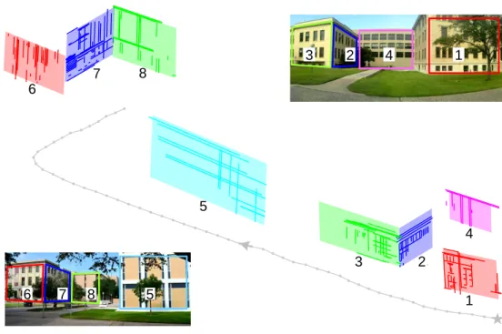
3.1 A sample output of high level landmarks and the robot trajectory after the mapping process in 3D view. The system is able to recognize primary planes from building facades and their corresponding co-planar lines as high level landmarks. The numbered corresponding building facades are also color coded in the top right and bottom left images. . . 10 3.2 (a) A illustration of the multilayer feature graph. (b) MFG structure. . . . 13 3.3 Uncertainty of line segment endpoints. . . 15 3.4 (a) A sample view (upper) and constructed 3D landmarks (lower). (b)

Standard deviations of plane depth vs #frames. . . 25 3.5 Experiment sites. . . 25 4.1 Sample result of our algorithm, and a Google EarthTMview of the same

site from a similar perspective. Coplanar landmarks (points and lines) are coded in the same color, while general landmarks are in gray color. The dotted line is the estimated camera trajectory. . . 29 4.2 The whole graph represents a 3D MFG, and the shaded regions jointly

rep-resent a 2D MFG. Geometric relationships between nodes are reprep-resented by edges of different line types. . . 33 4.3 System diagram. . . 36 4.4 An example of vanishing point matching. The line segments and ideal

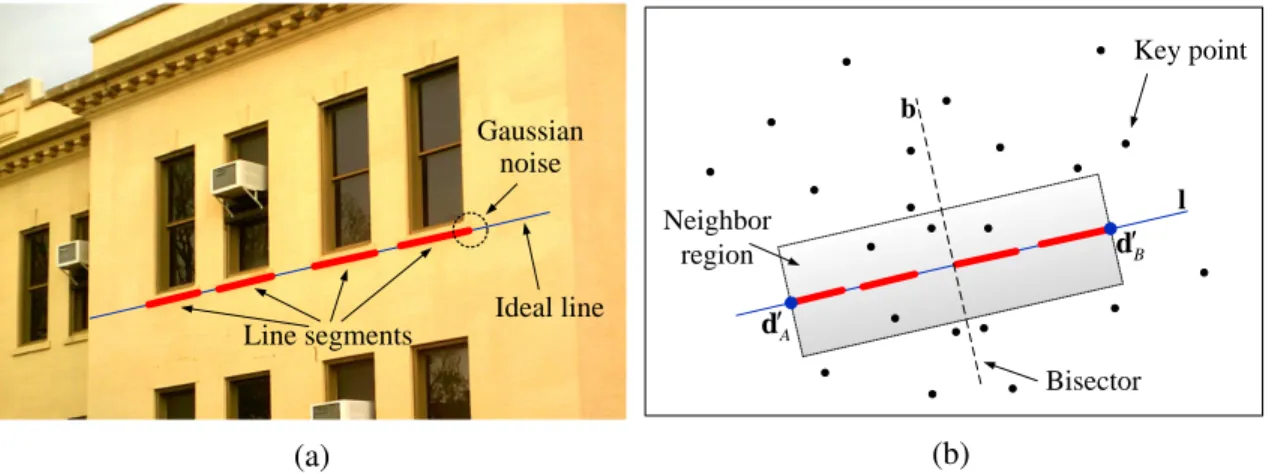
lines associated with the same vanishing points are drawn in the same color. 38 4.5 (a) An example of an ideal line. (b) An example of the adjacency between

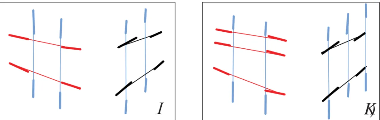
key points and ideal lines. . . 39 4.6 An example of our two-stage approach to ideal line matching. (a) and (b):

Ideal line matches found in Stage 1 by the PCLM method, each pair of line match is plotted in the same color, and small circles represent point correspondences used by PCLM; (c) and (d): Additional matches found by the FGLM method in Stage 2. (Best viewed in color) . . . 42

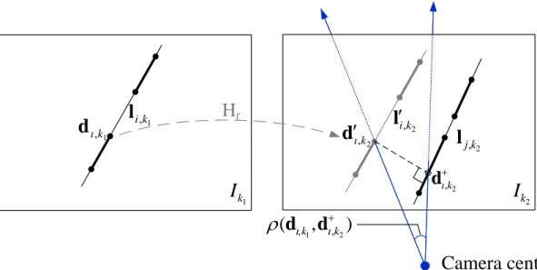
4.7 Illustration of parallax computation for 2D ideal lines. Hr is a rotational

homography defined in (4.7). Bold lines are supporting line segments of the underlying (thin) ideal line. ρ(dι,k1,d+ι,k2)is the parallax between pointsdι,k1 andd+ι,k2. . . 45 4.8 Sample images used for line matching test. . . 54 4.9 HRBB4 sequence. (a) Camera and robot. (b) Trajectory estimates aligned

with the ground truth using similarity transforms as described in (4.18). . 58 4.10 Contributions to LBA costs by different features. The costs are

dimension-less. . . 62 4.11 Estimated trajectories by our method for sequences 00 and 07 in the KITTI

dataset. . . 65 5.1 System diagram. . . 67 5.2 Sampling-based 3D line segment estimation. From a 2D line segment,ns

evenly-spaced points are sampled. The sample points are back-projected to 3D using depth information. Then a 3D line segment is fitted to these 3D points using RANSAC and Mahalanobis distance-based optimization. 74 5.3 Example of image brightness change over time under constant/varying

lighting (from Corridor-C). Here image brightness means the average in-tensity of an image. . . 86 6.1 A perspective illustration of the geometry relationship between real-virtual

pairs across two views. . . 96 6.2 The configuration of πI, πs, and πm. πs is placed to contain the camera

principal axis. . . 100 6.3 In-lab experiment setup. (a) Experiment configurations. (b) A sample view. 106 6.4 The accuracy of estimated mirror plane with respect toαvalues. (a)

Angu-lar error of the mirror normal. (b) Relative depth error for the mirror plane. The vertical bar and the middle cross represent the one standard deviation range and sample mean, respectively. . . 106 6.5 The mean and standard deviation plot of mirror plane parameters vs.

num-ber of quadruple inliers. (a) Angular error of the mirror normal. (b) Rela-tive depth error for the mirror plane. The vertical bar represents one stan-dard deviation range. . . 107

6.6 Sample images from the data set. . . 108

LIST OF TABLES

TABLE Page

3.1 Field mapping test results. . . 24

4.1 Ideal line matching results . . . 55

4.2 Parameter settings . . . 56

4.3 Absolute trajectory errors . . . 59

4.4 ATE’s (m) of HLVN variants . . . 61

4.5 Run time of HLVN . . . 63

4.6 Comparison on KITTI dataset . . . 65

5.1 TED (in meters) . . . 88

5.2 RMSE of RPE on TUM FR1 sequences . . . 89

1. INTRODUCTION

Robots are changing our life. Nowadays robots are not only operating in factories or outer space, but also participating in people’s daily activities. For example, by Feb. 2014 over 10 million Roomba robotic vacuums have been sold worldwide, cleaning rooms for people. Self-driving cars, which would greatly reduce traffic accidents and congestions, are getting closer and closer to real life, thanks to the continuous efforts of big companies like Google. Four U.S. states have passed laws permitting autonomous cars, including Nevada, Florida, California, and Michigan.

For any mobile robots, navigation is a fundamental capability. Robot navigation is a combination of multiple tasks including localization, mapping, motion planning, obstacle avoidance, etc. Localization and mapping answers two basic questions for a robot: “where am I” and “what is the world like”, respectively. Motion planning finds a path for a robot to move from its initial configuration to goal configuration. Obstacle avoidance keeps a robot from collision with objects.

Robot Navigation has been a popular research field in the past decades [1, 2]. For navigation, robots use sensors to perceive the world, including range sensors and passive sensors. Ultrasonic range sensors are inexpensive at the cost of low angular resolution. Laser range finders are expensive and not eye safe, despite high angular resolution. A common problem of range sensors is that they do not capture much information other than range, such as material and texture. On the other hand, cameras are not only inexpensive, but also able to capture rich texture and color information about the world. Meanwhile, cameras are becoming unprecedentedly available to everyone with the spread of mobile devices like cellphone and tablets. All these facts motivate us to study camera-based nav-igation, i.e., visual navigation.

In early robotics works, localization is conducted with respect to a map of known envi-ronment. As robotic sensors are inherently noisy, probabilistic approaches (e.g., Kalman filter) are widely adopted to solve the localization problem. However, when a robot ex-plores a previously-unknown environment with no map available, the chicken and egg problem arises: localization requires a known map, but mapping relies on accurate lo-cation information. This leads to the simultaneous localization and mapping (SLAM) problem, i.e., a robot constructs a map of an unknown environment while simultaneously keeping track of its own location within the map. For navigation in urban and indoor en-vironments, SLAM is especially important since GPS signals are often blocked/reflected by tall buildings.

SLAM has attracted extensive interest and research since early 1990’s. People have applied different kinds of sensors and proposed various techniques for SLAM. At present, laser-based SLAM algorithms can produce highly accurate results and are relatively ma-ture. On the contrary, visual SLAM (i.e. vision-based SLAM) is still facing a lot of challenges, despite its fast progress in the past decade.

The major challenge for visual SLAM lies in the robustness to lighting variation and feature distribution. The core element of visual SLAM algorithms is to estimate the rel-ative motion between two images based on commonly observed scene/objects. To do so, one needs to find out the correspondence between images, which can be either pixel-wise or between visual features such as interest points and edges. Unfortunately, the correspon-dence quality can be easily challenged by lighting variations and uneven feature distribu-tions, which directly degrades visual SLAM performance. For example, pixel-wise match-ing algorithms usually assume photo-consistency, which becomes invalid under lightmatch-ing change. Moreover, most visual SLAM algorithms are built upon a single type of visual feature for simplicity. However, when that type of feature is unevenly distributed or even absent in the scene, the estimation becomes subject to degenerated situations or failure.

Another limitation of current visual SLAM algorithms is that the resulted map is usu-ally composed of simple landmarks, which are constructed from low-level visual features. The most popular type of visual feature is points (also known as interest points or key points). While various point detection algorithms exist including SIFT, SURF and FAST, the generated map just consists of sparse point landmarks, without much semantic mean-ing. This hinders higher-level navigation tasks such as approaching an office door. It is thus desirable to build a map of higher-level landmarks such as planes or even objects. High-level landmarks can not only make a map more semantic but also enable more robust feature matching or place recognition.

To meet these challenges, we investigate feature fusion approaches in this dissertation. The basic rationale is that in urban and indoor environments there exist various feature types such points and lines, which have different properties; in combination, these features should improve the robustness of visual SLAM, and furthermore, high-level landmarks can be defined as or derived from their combinations, making maps more semantic.

We have designed a novel data structure, multilayer feature graph (MFG), which not only incorporates five types of features ranging from points to planes, but also models the geometric relationships between these feature types. We have prototyped MFG using a two view-based construction algorithm [3] to demonstrate its potential for facilitating visual navigation.

In this dissertation, we first extend the application of MFG to image sequence-based robotic mapping by using EKF. To be specific, we build a sequence of two view based MFGs from each pair of adjacent frames and analyze how errors are generated and propa-gated in the construction process of each MFG. We derive closed form solutions for error distributions, and the error analysis enables us to treat each MFG as an observation for the EKF at each iteration. Based on projective geometry of pinhole camera, we derive the observation models that complete the EKF framework. We have implemented the

EKF method and applied it to an automatic building exterior mapping task [4]. We have tested the algorithm using image data from outdoor man-made environments. Experiment results show that building facades are successfully constructed with mean relative error of plane depth less than 4.66%.

However, two view based MFG requires sufficient baseline to be successfully con-structed. This is not always feasible in real applications. This motivates us to devise a multiple view based algorithm to construct a single MFG which serves as a global map. As a result, our proposed heterogeneous landmark-based visual navigation algorithm takes a video stream as input, initializes and iteratively updates MFG based on extracted key frames; it also refines robot localization and MFG landmarks using local bundle adjust-ment [5, 6]. We present pseudo code for the algorithm and analyze its complexity. We evaluate our method and compare it with state-of-the-art methods using multiple indoor and outdoor datasets. In particular, on the KITTI dataset our method reduces the trans-lational error by 52.5% under urban sequences where rectilinear structures dominate the scene.

Monocular visual SLAM inevitably suffers scale drift due to depth ambiguity. This can be easily avoided by using an RGB-D camera, which provides pixel-wise depth mea-surements for color images. While most RGB-D SLAM algorithms use feature points, we investigate how to extract 3D lines from RGB-D data. More importantly, we propose an RGB-D odometry algorithm robust to lighting variation and uneven feature distribution by fusing point and line features. We extract 3D points and lines from RGB-D data, analyze their measurement uncertainties, and compute camera motion using maximum likelihood estimation. We prove that fusing points and lines produces smaller motion estimate un-certainty than using either feature type alone. In experiments our method outperforms the competing algorithms under both constant and varying lighting conditions.

and indoor environments, specular objects like mirrors challenge almost every type of robot sensors including laser range finds and sonar arrays. This is because light and sound signals simply bounce off the surfaces and do not return to receivers. We propose a method for this planar mirror detection problem using two views from an on-board camera [7]. We derive geometric constraints for corresponding real-virtual features across two views. We address an issue that popular feature detectors, such as scale-invariant feature transform (SIFT), are not reflection invariant by combining a secondary reflection with an affine scale-invariant feature transform (ASIFT). We employ a RANSAC framework to develop a robust mirror detection algorithm. The algorithm is tested under both in-lab and field settings, and it achieves an overall detection accuracy rate of 91.0%.

The rest of this dissertation is organized as follows. Section 2 reviews literature related to this dissertation. In Section 3, we present the MFG-based EKF framework and its application to building exterior mapping. Section 4 presents the heterogeneous landmark-based visual SLAM algorithm using multiple view landmark-based MFG. Section 5 presents our robust RGB-D odometry algorithm fusing point and line features. In Section 6, we report the planar mirror detection algorithm for obstacle avoidance. Section 7 concludes the dissertation and discusses future work directions.

2. LITERATURE REVIEW

Robot navigation is a combination of tasks including localization, mapping, motion planning, and obstacle avoidance. The works in this dissertation mainly relate to localiza-tion, mapping and obstacle avoidance.

Robotic localization is the problem of estimating robot poses (position and orientation) with respect to a given map. Because robotic sensors are inevitably subject to measure-ment noise, probabilistic approaches are widely adopted for localization, such as EKF [8], probability grids [9], and particle filter [10]. When navigating in unknown environments, localization and mapping have to be conducted in the same time, which is known as the simultaneous localization and mapping (SLAM) problem. A solution to the SLAM prob-lem is considered as the key for mobile robots to be truly autonomous. Early works [11] show that a consistent solution of SLAM requires a joint estimate of the robot poses and every landmark. Later on people further realize that SLAM is actually a convergent prob-lem [12]. Representative approaches to the SLAM probprob-lem include EKF-based , particle filter-based (e.g. FastSLAM [13]), and information filter-based [14] methods.

Visual SLAM.Various types of sensors have been applied to SLAM, including

ultra-sonic sensors, Lidar, cameras. The works in this dissertation utilize cameras primarily, and thus belong to the visual SLAM category. Visual SLAM is also commonly referred to as structure from motion (SFM) or visual odometry in computer vision domain. In this dissertation, we consider these terms to be interchangeable. There exist two prevalent cat-egories of approaches for visual SLAM, one based on sequential filtering (e.g. [15]) with its root in the traditional SLAM research, the other based on bundle adjustment (BA) [16] which is a standard optimization technique in computer vision. BA essentially estimates

all camera poses and landmark parameters in a big nonlinear optimization problem, which is usually computationally expensive. Local bundle adjustment is a technique proposed to allow online processing by limiting the camera poses and landmarks to be within a window of latest frames.

The basic element of a typical visual SLAM system is pairwise motion estimation, i.e. recovering the relative 3D rigid transformation between two camera frames. This can be solved by using either pixel-to-pixel registration (i.e. dense methods) or sparse feature matches. Compared with dense methods, sparse features are less sensitive to perspective and/or illumination changes. Various interest point feature detection and/or description algorithms have been adopted in visual SLAM such as SIFT [17] and speeded-up robust feature (SURF) [18]. Other feature types are also studied for visual SLAM, such as line segments [19–22], straight lines [23], vanishing points [24], and planes [25–28]. However, points are still the most commonly used feature due to its simplicity; moreover, most visual SLAM works are built on a single feature type. As a result, existing methods are not very robust to large lighting variations and uneven feature distributions. The works in this dissertation focus on exploiting the combinational power of different feature types in order to achieve better accuracy and robustness. We propose a novel data structure to organize different types of visual features, based on which we respectively develop EKF-based and LBA-based visual SLAM algorithms and evaluate them using real-world data.

RGB-D odometry. A regular RGB camera only measures angular information of

objects, with the depth information missing. This produces a scale ambiguity in monocular visual SLAM, and further results in the notorious scale drift problem [29]. The recent emergence of RGB-D cameras (e.g. Microsoft Kinect) solves the scale ambiguity/drift issue to a great extent. This is because RGB-D cameras provide pixel-wise depth data for every color image. To perform SLAM using RGB-D data, point cloud registration methods (e.g. ICP [30]) can be applied [31], but they are easily hindered by degenerated

cases. Traditional visual SLAM algorithms are also applicable to RGB-D SLAM with slight modifications [32, 33], which are still sensitive to lighting variations and uneven feature distribution. Our work investigates how to fuse point and line features in RGB-D SLAM to improve the system robustness. We prove that this feature fusion approach produces smaller estimation uncertainty than using either feature alone.

Obstacle avoidance.Besides localization and mapping, obstacle avoidance is another

important research problem in navigation. To cope with this problem, range data from ultrasonic [34] or laser [35] range finders are commonly used to detect obstacles. In general range sensors are able to reliably detect normal obstacles like chairs and boxes, except for specular surfaces (e.g. mirrors). This is because sound or light does not return to the receivers after specular reflections most of the time. Our work detects planar mirrors using a vision-based algorithm. Our algorithm not only detects the existence of planar mirrors, but also estimates their poses relative to the camera.

3. AUTOMATIC BUILDING EXTERIOR MAPPING USING MULTILAYER FEATURE GRAPH AND EXTENDED KALMAN FILTER*

We are developing visual algorithms to assist building exterior survey using a mobile robot, which can greatly assist building energy retrofitting. The task requires a robot to map building facades with its on-board camera while the robot travels. Existing naviga-tion methods often utilize low level landmarks, such as feature points and point clouds, and cannot directly provide information for build facades, which can be viewed as high level landmarks. Actually, the high level landmarks, such as primary planes and salient lines, have distinctive advantages over low level features. Bearing clear geometric mean-ing, high level landmarks are less sensitive to different lighting conditions and varying shadows where low level features are often challenged. High level landmarks are ubiq-uitous in modern urban areas where rectilinear objects dominate camera field of view. Humans are used to navigating in unknown environments by effectively using high level landmarks as reference. However, robots still have difficulty to utilize advantages of high level landmarks due to challenges in feature recognition and correspondence.

In 2012, we [3] proposed a two-view MFG (multilayer feature graph) as a scene un-derstanding and knowledge representation method for robot navigation. An MFG is con-structed from overlapping and dislocated two views and contains five different features ranging from raw key points to planes and vanishing points in 3D. Here we build our high level landmark-based maps (see Fig. 3.1) by employing MFG as observations in an EKF framework. We analyze how errors are generated and propagated in the MFG construc-tion process, which characterizes observaconstruc-tion errors in the EKF. We derive closed form *Reprinted with permission from “Automatic building exterior mapping using multilayer feature graphs” by Y. Lu, D. Song, Y. Xu, A. G. A. Perera, and S. Oh, 2013. IEEE International Conference on Automation Science and Engineering (CASE), pp. 162-167, Copyright c2013 IEEE.

1 2 4 3 5 6 7 8 1 3 2 4 5 6 7 8

Figure 3.1: A sample output of high level landmarks and the robot trajectory after the mapping process in 3D view. The system is able to recognize primary planes from building facades and their corresponding co-planar lines as high level landmarks. The numbered corresponding building facades are also color coded in the top right and bottom left images.

solutions for error distributions. Based on projective geometry, we derive the observation models to complete the EKF framework. We have implemented and tested our MFG-EKF method at three different sites. Experimental results show that high level landmarks are successfully constructed in modern urban environments with mean relative plane depth errors less than 4.66%.

3.1 Related Work

Robotic mapping with high level landmarks relates to a broad body of research in SLAM and visual odometry including different sensor configurations and different land-mark selections.

com-mon sensors for robot navigation include sonar arrays [1], laser range finders [36, 37], depth cameras [32], regular cameras [38, 39] , or their combinations [40, 41]. Mapping tasks are often conducted under the SLAM framework [42]. As a partially observable Markovian decision process, SLAM infers system states based on the sensory input using different filters and loop closure techniques. The system states usually include both land-marks and robot states whereas landland-marks are the representation of the physical world. For example, landmarks are point clouds if a laser ranger finder or a depth camera is the primary sensor. In vision-based SLAM, SIFT feature points or its variants [15] and line features [19, 23] are often employed as landmarks.

Our work belongs to the vision-based SLAM category where one or more cameras are the primary navigation sensor. Recently, many researchers realize landmark selections can make a difference in SLAM and visual odometry performance. Lower level land-marks [15], such as Harris corners and SIFT points, are relatively easy to use due to their geometric simplicity, which share many geometric properties with traditional point clouds used for laser range finders. However, point features are merely mathematical singulari-ties in color, texture, and geometric space. They can be easily influenced by lighting and shadow conditions. Realizing the limitation, recent efforts focus on developing high level landmarks such as lines/edges/line segments [20, 22]. Zhang et al. [43] use vertical lines and floor lines in a monocular SLAM and build a 3D line-based map in an indoor corridor environment.

More recent sophisticated methods combine multiple features such as points, lines, and planes. Gee et al. [25] incorporate 3D planes and lines into visual SLAM framework. Martinez et al. [26] propose a monocular SLAM algorithm that unifies the estimation of point and planar features. These works have demonstrated the robustness of high level landmarks and inspired this work. Observe that the existing works only treat different landmarks as isolated geometric objects, without exploring the inner relationship between

them. The treatment simplifies the SLAM problem formulation but cannot fully utilize the power of high level landmarks.

3.2 Problem Definition

Consider a robot equipped with a single camera navigates in an unknown environment. The robot attempts to estimate high level landmarks such as building facades or salient edges from input image frames. The basic assumptions are,

a.1 The robot operates in a largely static modern urban environment with rectilinear structures, which is the prerequisite for MFG.

a.2 The onboard camera is pre-calibrated and has a known intrinsic matrixK.

a.3 The initial step of robot movement is known for reference. Otherwise, estimates would be up to scale. The assumption can be relaxed if a stereo camera is available. In our approach, adjacent raw image frame pairs are first employed to construct MFG [3] sequence. Let Ik be thek-th (k ∈ N) image frame and Mk (k ≥ 1) be the MFG con-structed from framesIkandIk−1. Fig. 3.2 illustrates that MFG is a data structure composed

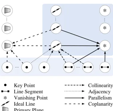
of five layers of feature nodes: key points,line segments, ideal lines, primary planesand vanishing points; edges between nodes of different layers represent geometric relation-ships includingadjacency,collinearity,coplanarity, andparallelism.

The resulting MFG sequence,{Mk, k ≥1}, is considered as the input to the problem. Denote{Ck}the camera coordinate system (CCS) associated withIk. MFGs assist us in identifying high level landmarks such as 3D planes and their associated coplanar lines in physical space. However, the planes and lines fromMkare represented w.r.t.{Ck}, which cannot be directly used as global landmarks. Define the world coordinate system (WCS),

(a) collinearity primary planes vanishing points ideal lines line segments key points parallelism coplanarity adjacency p1 pi s1 l1 si+1 sm pi+1 pn li li+1 lq si πp πi π1 vv v1 v2 (b)

Figure 3.2: (a) A illustration of the multilayer feature graph. (b) MFG structure.

Definition 1. Given MFG sequence {Mk : k ≥ 1, k ∈ N}, map high level landmarks

including 3D planes and coplanar lines in{W}, and assess the uncertainty of the mapping process by deriving error covariance matrices for each landmark.

To solve the landmark mapping problem, we employ an EKF-based approach. In this approach, MFGMkcan be considered as a generalized observation at timek. Therefore, we need to understand how errors are distributed in the construction process ofMk, which can serve as the observation error in the EKF. With the observation error derived, the landmark errors can be estimated by combining process errors using the EKF. Therefore, the problem is solved in two steps with the first step being the uncertainty analysis of MFG.

3.3 Observation Error: Uncertainty in MFG

Our previous work [3], has shown how to construct MFG using a feature fusion method. However, the uncertainty of each feature layer is yet to be analyzed. Here we detail the uncertainty for each layer of MFG in a bottom-up manner.

3.3.1 Error Modeling of Raw Features

The MFG construction algorithm takes two images I and I0 as input and outputs a feature graph of five layers, as illustrated in Fig. 3.2(b). In MFGs, key points and line seg-ments are raw features directly detected from images using SIFT [17] and LSD [44], while ideal lines, primary planes and vanishing points represent high level features constructed from raw features. MFGs also include feature correspondences between two views.

Note thatI and I0 actually represent Ik and Ik−1 in the continuous image sequence,

respectively. Here we drop k andk −1from notations for simplicity. Furthermore, we attach a superscript0to variables associated withI0. As a convention, we use a∼on top of a homogeneous vector to denote its inhomogeneous counterpart throughout this section.

For each key pointpi in I, we model its measurement error as an independent and identically distributed (i.i.d.) zero-mean isotropic Gaussian noise with varianceσ2 in each axis

Cov(˜pi) =σ2I2, ∀i (3.1)

whereI2is a2×2identity matrix.

For each line segmentsi inI, denote its two endpoints byei1 andei2. Defineuik and

ui⊥to be two unit vectors parallel and perpendicular to the line segment, respectively (see

Fig. 3.3). We model the error ofei1(the same forei2) as an independent 2D Gaussian with

its covariance matrix to be diagonal in the coordinate system defined by uik and ui⊥ as

below Σik⊥ =    σ2 ik 0 0 σ2 i⊥   , (3.2)

whereσi⊥ andσik are the standard deviations ofei1 in directions ofui⊥ anduik,

respec-tively. σi⊥is usually much smaller thanσik. We have observed thatσi⊥usually is inversely

 i   i u ei2 ei1 ui|| ϕi _u v | | i 

Figure 3.3: Uncertainty of line segment endpoints.

to pixelization error. Thus, we model the endpoint error as follows,

σik =σk, σi⊥=

σik

ksik

+σp, ∀i, (3.3)

whereσkandσpare constant and independent ofi, andksikdenotes the length ofsi. The

parameters for the models can be determined using Monte Carlo simulation. Projecting (3.2) back to the image coordinate system (ICS), we have

Cov(˜ei1) = R(φi)Σik⊥R(φi)T (3.4)

whereφiis the angle betweenuik ( Fig. 3.3) andu-axis, andR(φi) =



 

cosφi −sinφi

sinφi cosφi



 .

Note that the error model in (3.2-3.4) for line segments may differ for different line detec-tors. However, the rest of our analysis still applies.

With error distributions of raw features obtained, we are ready to analyze high level features such as ideal lines and primary planes.

3.3.2 Error Analysis of Ideal Lines

In the MFG construction process, an ideal lineli is obtained by fitting a straight line through endpoints of a set of mi collinear line segments {sj : 1 ≤ j ≤ mi}. The i-th ideal line inIcan be parameterized in terms of angleθiand interceptρiwith the following homogeneous format in ICS,

li = [cosθi,sinθi, ρi]T (3.5)

such thatucosθi+vsinθi+ρi = 0holds for any point(u, v)onli. Since the fitting process employs maximum likelihood estimation (MLE) to obtain optimal solution [θ∗_i, ρ∗_i]T, we have the following lemma.

Lemma 1. Given collinear line segments set{sj}with their endpoint covariance matrices

in (3.4), if MLE is employed to estimate[θ∗_i, ρ∗_i]T_{, the resultingl}

i can be approximated by a Gaussian with a mean vector of[cosθ_i∗,sinθ∗_i, ρ∗_i]T_{and a covariance matrix of,}

Cov(li) =J Cov(θi∗, ρ ∗ i)J T , (3.6) whereJ =    −sinθ_i∗ cosθ∗_i 0 0 0 1    T

and Cov(θ∗_i, ρ∗_i)is given by (3.9).

Proof. Let us formulate this MLE problem first. This MLE problem simultaneously seeks for line parameters [θi, ρi]T and the corrected line segment endpoints, denoted by ejτ, τ = 1,2. To ensureeT_jτli = 0, we use the parametrization

˜

e_jτ(tjτ) =



 

−ρicosθi

−ρisinθi   +tjτ    sinθi −cosθi    (3.7)

wheretjτ ∈Ris the only free parameter for˜ejτ that we need to estimate.

Define a parameter vector that is to be estimated as ΘL = [ΘTL1,ΘTL2]T with ΘL1 =

[θi, ρi]T andΘL2 = [t11, t12,· · · , tmi1, tmi2]

T_{. Define a measurement vector that}

incorpo-rates measurement data asΩL = [˜eT11,˜eT12,· · ·,e˜Tmi1,˜e

T

mi2]

T_{. Define a measurement}

func-tionfL(·)that maps from parameter space to measurement space, which is straightforward to be obtained from (3.7).

The MLE problem now becomes

arg min ΘL (ΩL−fL(ΘL))TΣΩ−1L(ΩL−f(ΘL)), (3.8) where ΣΩL =       Cov(˜e11) 0 . .. 0 Cov(˜emi2)       2mi×2mi .

The above optimization problem can be solved by the Levenberg-Marquardt algorithm (LMA). Denote the optimal estimate by [Θ∗T

L1,Θ ∗T L2]T. The covariance of[θ ∗ i, ρ ∗ i]Tcan be computed following the method in Chapter 5 of [45] as below

Cov(Θ∗_L1) = (U −W V−1WT)†, (3.9) whereU =AT_Σ−1 ΩLA,V =B T_Σ−1 ΩLB,W =A T_Σ−1 ΩLB, A=∂fL/∂Θ∗L1, B =∂fL/∂Θ∗L2,

and()†indicates the pseudo-inverse operation.

Due to the fact that endpoints of line segments are conformal to independent Gaussian distributions, the property of MLE ensures that [θ_i∗, ρ∗_i]T _{is asymptotically normal (Thm.}

3.1 in pp. 2143 of [46]). Hence we can use a 2D Gaussian to approximate its distribution. Furthermore, through error forward propagation approximation, we arrive at (3.6). Lem. 1 is proved.

3.3.3 Error Analysis of Primary Planes

In an MFG based on two views, a primary plane πi is a 3D plane represented by a 4D homogeneous vector in the CCS associated with I. Furthermore, if πi does not pass through the camera center (which is often the case in practice), we can have

πi = [ ˜πTi ,1]

T_,

(3.10)

whereπ˜iis a3×1vector for the inhomogeneous representation ofπi.

Based on the coplanarity relationship in an MFG, each planeπican be associated with pi coplanar point correspondences {pij ↔ p0_ij : j = 1,· · · , pi}, and qi coplanar line correspondences {liκ ↔ l0iκ : κ = 1,· · · , qi}. These feature correspondences satisfy a homography induced byπi p0_ij = Hipij , liκ= HTil 0 iκ, (3.11) where Hi =K(R−tπ˜iT)K −1 , (3.12)

andRandtare the rotation matrix and translation vector between two views, respectively. Eqs. (3.11 and 3.12) suggest a method of computingπ˜i based onRandt. However, if

Randtare simply derived from epipolar geometry without considering the planar struc-ture information, the solution is not optimal, and neither is π˜i. Inspired by the method from [47], we estimate allπ˜i’s, Randtsimultaneously by employing all geometric

fea-tures (i.e., key points and ideal lines) and constraints (i.e., epipolar constraint and homog-raphy) under an MLE framework. Define ΘP1 = [ ˜πT1,· · · ,π˜Ti ,· · ·]T. SupposingΘ

∗

P1 is

the MLE output ofΘP1, we have the following lemma.

Lemma 2. Given that key point errors follow i.i.d. isotropic Gaussian distributions with

covariance matrices in (3.1) and line segment endpoints follow independent Gaussian distributions with covariance matrices in (3.4), if MLE is employed to estimate all π˜i’s for primary planes, then the distribution of each π˜i can be approximated by a Gaussian distribution with the following mean and covariance matrix,

˜

π_i∗ =TiΘ∗P1 (3.13)

Cov( ˜π_i∗) =TiCov(Θ∗P1)T

T

i (3.14)

where Ti = [03,3i−3 : I3 : 03,3(p−i)+6], Cov(Θ∗P1) is derived in a way similar to that in

(3.9),0a,bis ana×bzero matrix, andI3is a3×3identity matrix.

Proof. Similar to the proof of Lem. 1, let us formulate the MLE problem first. This MLE problem estimates planes (π˜i’s), relative pose (Randt) as well as corrected feature corre-spondences simultaneously. Define a measurement vector

ΩP = [· · · ,p˜Tij,p˜

0T

ij,· · · , θiκ, ρiκ, θ0iκ, ρ

0

iκ,· · · ,p˜Tr,p˜

0T

r ,· · ·]T

where[θi, ρi]are the parameters ofli, and{p˜r ↔p˜0r :r ≥1}denote the point correspon-dences that are not associated with any plane,

and a parameter vectorΘP = [ΘTP1,ΘTP2]Twith

ΘP2 = [α, β, γ,tT,· · · ,p˜Tij,· · · , θ 0 iκ, ρ 0 iκ,· · · ,P˜ T r,· · ·] T , 19

whereα, β andγ are the Euler angles ofR,P˜r is the 3D point corresponding topr. Now, we define the measurement function for each type of feature correspondence accordingly as below.

• for point correspondences on planeπi:

˜ pij = ˜pij, p˜0ij = (Hipij)1:2 (Hipij)3 , whereHiis defined in (3.12).

• for line matches on planeπi:First, let us define a function

g(l) = [θ, ρ]T (3.15)

that maps a line vectorl= [cosθ,sinθ, ρ]T_{to its parameters. Now the measurement}

function for line correspondences is

   θ_iκ0 ρ0_iκ   =    θ_iκ0 ρ0_iκ   ,    θiκ ρiκ   =g HT il 0 iκ k(HT i l 0 iκ)1:2k .

• for point correspondences not on any plane:

˜ pr = (PPr)1:2 (PPr)3 , p˜0_r = (P 0_P r)1:2 (P0_P r)3 , whereP =K[ I3|0 ],P0 =K[ R|t].

The MLE problem is formulated the same as (3.8) except thatΣΩP is obtained from

(3.1) and (3.9). Let the optimal estimate beΘ∗_P = [Θ∗_PT₁,Θ_P∗T₂]T. Cov(Θ∗_P1)can be com-puted in the similar way as in (3.9). Since the rest of the proof is similar to that in the proof of Lem. 1, we skip the details here. Hence Lem. 2 is proved.

3.4 EKF based Mapping with MFG

Two-view based MFGs only provide local information of high level features. In order to build a global map in{W}, EKF is employed to estimate the posterior of landmarks as well as a robot trajectory.

3.4.1 System State Representation

In the EKF framework, we maintain and keep updating a system stateyk, which is composed of the robot statexkand 3D landmarks.

The robot state is defined as

xk = [rTk,q T k,ν T k,ω T k] T_, (3.16)

where rk is a 3D location in {W}, qk is an orientation quaternion w.r.t. {W}, νk is a velocity vector in{W}, andωkis an angular velocity vector in{Ck}.

In yk, we use π˜_iW to represent thei-th 3D plane landmark in {W}. To represent a 3D line, general methods like Pl¨ucker coordinates would need as many as 6 parameters. However, a 3D vector is sufficient in this work since our method is only interested in coplanar lines associated with landmark planes. Supposing a landmark line resides on planeπ˜W

i , then there exists an one-to-one mapping between this line and its projection on image planeI0, which is actually a 2D homography induced by π˜Wi . Let us denotelkj the projection of thej-th landmark line onIk. Then, we can usel0j to fully represent thej-th landmark line inyksince we already haveπ˜iW inyk.

As a result, the complete system state can be written as

yk =

xT_k,· · ·,( ˜π_iW)T,· · · ,(l0_j)T,· · ·T. (3.17)

3.4.2 EKF Formulation

In an EKF framework, a process model and an observation model need to be specified for the prediction and update steps, respectively.

3.4.2.1 Process Modeling

We follow the conventional assumptions of “constant velocity, constant angular veloc-ity” in [15] for camera motion to formulate the process model as follows,

xk+1 =          rk+1 qk+1 νk+1 ωk+1          =          rk+νk∆t qk×q(ωk∆t) νk ωk          ,

where q(ωk∆t) denotes the quaternion defined by the angle-axis rotation vector ωk∆t, and ∆t is the time interval between two steps. Note this is just a partial model for the system state in (3.17) while the rest of states ofyk are landmark states. Since landmarks are assumed to be static, their corresponding states remain unchanged in the prediction step.

3.4.2.2 Observation Modeling

An observation function maps the system state to landmark observations. For a plane landmarkπ˜_iW, the observation produced byMkis its representationπ˜ikin{Ck}. Define a matrixW_k T that transforms a 3D point (of homogeneous format) from{Ck}to{W}as

W k T =    R(qk) rk 0 1    4×4 , (3.18)

whereR(qk)represents the rotation matrix defined byqk. For a primary plane landmark

πk

i, we know thatπki =Wk TTπiW. This implies the observation to be

˜ π_ik= W k TTπiW 1:3 W k TTπiW 4 (3.19)

where(V)adenotes thea-th element of vectorV, and(V)a:b denotes the sub vector of V indexed fromatob.

For a line landmarkl0

j, its observation fromMkislkj. Supposingl0j lies on planeπ˜iW, lk

j can be computed froml0j via a homography [45] lk_j = (H k i)−Tl0j (Hk_i)−Tl0_j 1:2 (3.20) whereHk_i =K h R−1(qk) +R−1(qk)rk π˜W_i T i K−1 andk · kisL2norm.

Eqs. (3.19 and 3.20) fully determine the observation function. It is worth noting that the covariance matrices of observation noise have been presented in Lems. 1 and 2. EKF also provides covariance of landmarks in its covariance update and prediction steps. Since this is a standard EKF procedure, we skip details here.

3.4.3 Landmark Initialization and Management

Since two views are needed to establish an MFG, the system should start atk = 1

when M1 is constructed and landmark planes and lines are added to y1. Starting from

y1, the system enters the prediction and update loops. As the robot travels farther, new

landmarks may be discovered and added to the system state. Because the MFG output is the landmark representation in the current CCS, it needs to be transformed to{W}before augmenting the system state. This coordinate transformation is represented byW_k T or the inverse ofHk

i as shown in (3.18-3.20).

3.5 Experiments

We have implemented the proposed method using Matlab on a Desktop PC. The cam-era used in the experiment is a pre-calibrated Nikon D5100 camcam-era equipped with a 18 mm lens, which ensures a horizontal field of view of60◦. Images are down-sampled to a resolution of800×530pixels. We have conducted two experiments: uncertainty test and field mapping test.

3.5.1 Uncertainty Test

The purpose of this experiment is to verify how the estimation uncertainty of landmarks changes as more images entering our system. A sequence of 14 images has been taken while the camera was carried by a person walking towards a building. The starting point is around 40 meters away from the building. Images have been captured every1∼2meters approximately with the first step length known to be 1.5 meters.

The upper image in Fig. 3.4(a) shows a sample of the image sequence and the lower line drawing in Fig. 3.4(a) shows the 3D landmarks constructed from the image sequence. Each plane and its coplanar line segments are coded in the same color. Fig. 3.4(b) demon-strates that the standard deviation of the depth of each landmark plane (using the same color coding as that in the lower line drawing in Fig. 3.4(a) decreases as the frame number increases.

3.5.2 Field Mapping Test

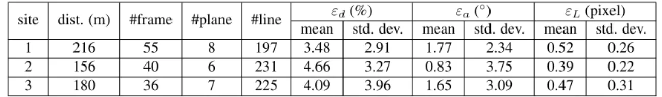
Table 3.1: FIELD MAPPING TEST RESULTS. site dist. (m) #frame #plane #line εd(%) εa(

◦_{) ε}

L(pixel)

mean std. dev. mean std. dev. mean std. dev.

1 216 55 8 197 3.48 2.91 1.77 2.34 0.52 0.26

2 156 40 6 231 4.66 3.27 0.83 3.75 0.39 0.22

X Z Y 1 2 3 4 5 6 7 8 9 10 11 12 13 0.5 1.0 2.0 1.5 Frame P la n e d e p th s ta n d a rd d e v ia ti o n ( m )

(a)

(b)

(a)

(b)

Figure 3.4: (a) A sample view (upper) and constructed 3D landmarks (lower). (b) Standard deviations of plane depth vs #frames.

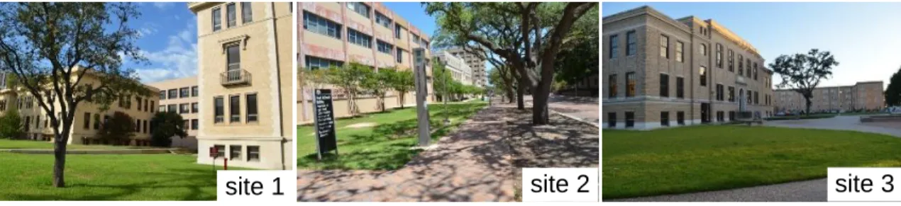
In the second experiment, we have tested our method in the field including three sites on Texas A&M University campus as shown in Fig. 3.5. At each site, the camera follows a pre-defined route. Images are taken every 4 meters approximately while the first step has been known to be exact 4.0 meters as a reference. The distance traveled and the numbers of frames collected at each site are shown in columns 2 and 3 of Tab. 3.1. As shown in the table, our method was able to successfully recognize high level landmarks including

site 1 site 2 site 3

Figure 3.5: Experiment sites.

primary planes (col. 3) and their coplanar line segments (col. 4). Fig. 3.1 actually shows a 3D visualization of the map of high level landmarks constructed from data of site 1, where coplanar lines are color coded according to underlying planes.

We employ three error metrics to assess landmark mapping accuracy. εd and εa are defined for evaluating planes, andεLis defined for assessing lines. Suppose planeπ˜Wi is introduced to the map since theki-th frameIki. Letdi denote the true plane depth ofπ˜

W i in{Cki}obtained using a BOSCH GLR225 laser distance measurer with a range up to 70

m and measurement accuracy of ±1.5 mm. Definediˆ as the estimated value of di from EKF output. Then a relative metric for plane depth error is defined as

εd= 1 N N X i=1 kdi−dˆik di , (3.21)

where N is the number of landmark planes. Similarly, define εa to be the angular error metric for plane normal. It is worth noting that there exists global drifting error between

{Cki}and{W}, which will be addressed in future loop closure stage. Here we focus on

εdandεaafter the plane landmark appears in the camera field of view.

To evaluate a line landmark’s estimation accuracy, we consider a re-projection error in ICS. Supposel0_j is added to the map since thekj-th frame. Letˆlkj be the re-projection ofl0_j inIkj, ande

(j)

h be theh-th observed endpoint of line segment inIkj associated with

ˆ_lk

j. Then the error metric for lines is defined based on the distance between observed line segment endpoints and re-projected line in local frame:

εL = 1 M M X j=1 1 Nj Nj X h=1 d⊥(e(_hj),ˆlkj), (3.22)

whered⊥(·)represents the distance from a point to a line,M is the number of line

Tab. 3.1 shows the mapping results based on the three metrics. It is clear that our method successfully maps the high level landmarks. However, since loop closure has not been performed, the estimated camera trajectory inevitably suffers from drifting error, which will be addressed in the future work.

3.6 Conclusions

We developed a method to allow a mobile robot to perform mapping of building fa-cades by enabling high level landmark mapping. The method incorporated a multiple layer feature graph into an EKF framework. We analyzed how errors are generated and propa-gated in the MFG construction process, which are used as observation error models in the EKF. We derived closed form solutions for error distribution to quantify the observation errors. Based on projective geometry, we derived observation models to complete the EKF framework. We implemented and tested the system at three different sites. Experiment re-sults have shown that high level landmarks are successfully constructed in a modern urban environment with mean relative plane depth error less than 4.66%.

4. VISUAL NAVIGATION USING HETEROGENEOUS LANDMARKS AND UNSUPERVISED GEOMETRIC CONSTRAINTS*

While the MFG-EKF method in Section 3 is able to map the building facades from image sequences, the camera trajectory estimation is subject to obvious drifting as the travel distance increases. One reason is that the linearization step in EKF leads to incon-sistencies due to the high nonlinearity in projective camera models. Recent studies [4] show that bundle adjustment-based SLAM approaches can produce better accuracy than EKF-based methods. Another limitation of the MFG-EKF method is its dependence on two view-based MFG. However, two view-based MFG needs a sufficient baseline, which is not always feasible. This motivates us to design a multiple view based MFG algorithm for visual SLAM using bundle adjustment.

In this section, we continue utilizing heterogeneous visual features and their inner geometric constraints to assist robot navigation, which is managed by a multiple view based MFG. Our method extends the local bundle adjustment-based SLAM framework by explicitly exploiting heterogeneous features and their geometric relationships in an unsu-pervised manner. The proposed heterogeneous landmark-based visual navigation (HLVN) algorithm takes a video stream as input, initializes and iteratively updates MFG based on extracted key frames, and refines robot localization and MFG landmarks. We present the algorithm pseudo code and analyze its complexity. We evaluate our method and compare it with state-of-the-art methods using multiple indoor and outdoor datasets. In particular, on the KITTI dataset our method reduces the translational error by 52.5% under urban sequences where rectilinear structures dominate the scene.

*Reprinted with permission from “Visual navigation using heterogeneous landmarks and unsupervised geometric constraints” by Y. Lu and D. Song, 2015. IEEE Transcations on Robotics, vol. 31, no. 3, pp. 736-749, Copyright c2015 IEEE.

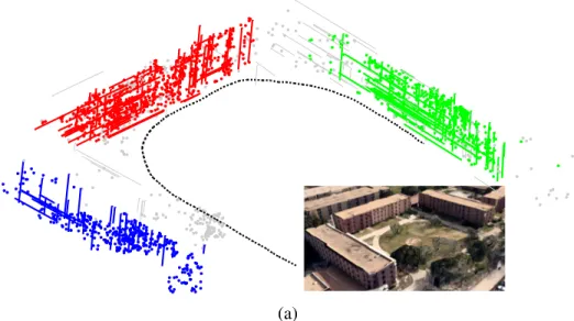
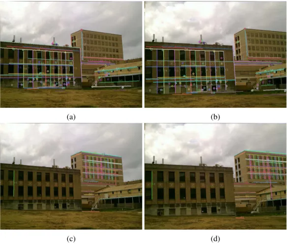
(a)

Figure 4.1: Sample result of our algorithm, and a Google EarthTMview of the same site from a similar perspective. Coplanar landmarks (points and lines) are coded in the same color, while general landmarks are in gray color. The dotted line is the estimated camera trajectory.

4.1 Related Work

Visual navigation using heterogeneous landmarks mainly relates to two research fields: 3D reconstruction and SLAM.

In computer vision and graphics, 3D reconstruction has been a very popular topic for research as well as commercial applications. Besides regular cameras, sensors used for 3D reconstruction also include laser range finder [48] and more often, aerial cameras [49]. Google Earth and Microsoft Virtual Earth are successful showcases for 3D reconstruc-tion of city models [50]. Following the taxonomy of Seitz et al. [51], 3D reconstrucreconstruc-tion algorithms are categorized into the following classes: voxel approaches [52], level-set techniques [53], line segment matching [54], polygon mesh methods [55], and algorithms that compute and merge depth maps [56]. Unlike those methods, our work does not pur-sue a full scale reconstruction. This is because 3D reconstruction usually needs repetitive

scene scanning, which is often not the main task for robots.

In robotics research, the most common external sensors for robot navigation include sonar arrays, laser range finders, GPS, cameras and their combinations. SLAM is the typical framework employed in robot navigation [42, 57]. In SLAM, the physical world is represented as a collection of landmarks. For example, point clouds serve as landmarks when a laser range finder is the primary sensor [58]. In particular, our work belongs to the visual SLAM category, where cameras provide the main sensory input [59–62].

There are two prevalent methodologies in visual SLAM: the bundle adjustment (BA) approaches (e.g., [59]) rooted in the structure from motion area in computer vision, and the filtering methods (e.g. [15]) originated from the traditional SLAM field of robotics research. Strasdat et al. have analyzed the advantages of each method in [63]. For both methods, various camera configurations/modalities have been studied, including a monoc-ular camera [64], a stereo camera [39, 65, 66], an omnidirectional camera [67], a camera with range sensors [68, 69], and an RGB-D camera [32, 70].

Besides methodology and sensor configuration, another critical issue in visual SLAM is scene representation. For example, point clouds and sparse feature points [71] are often employed as landmarks in a map. Recently, many researchers have realized that landmark selection is an important factor in visual odometry and SLAM [72]. Lower level landmarks such as corners [73] and SIFT points [17] are relatively easy to use due to their geometric simplicity. However, point features are merely mathematical singularities in color, texture and/or geometric spaces. They are difficult to interpret and use for scene understand-ing or human-robot interaction. They are also easily influenced by lightunderstand-ing and shadow conditions. To overcome these shortcomings, higher level landmarks have received more and more attention for visual SLAM, such as line segments [19–22], straight lines [23], vanishing points [24], and planes [25–28].

robust-ness and accuracy, but they either treat these landmarks as isolated objects, or partially explore the inner relations between them. This treatment simplifies the SLAM problem formulation but cannot fully utilize the power of heterogeneous landmarks. Very recently, Tretyak et al. present an optimization framework for geometric parsing of image by jointly using edges, line segments, lines, and vanishing points [74]. However, this method has not been applied to navigation yet.

4.2 Problem Formulation 4.2.1 Assumptions and Notations

Consider a mobile robot navigating in a previously unknown environment with a monoc-ular camera. We make two assumptions here:

a.1 The robot operates in a largely static man-made environment with rectilinear struc-tures consisting of parallel lines which are not necessarily in orthogonal directions.

a.2 The camera is pre-calibrated with its radial distortion removed. Let us define the following notations,

V Input camera video,

Ik k-th key frame extracted fromV,Ik ∈ V, k ∈N,

{Ck} 3D camera coordinate system forIk, a right-handed coordinate system with its ori-gin at the camera optical center, itsZ-axis coinciding with the optical axis and point-ing to the forward direction of the camera, and itsX-axis andY-axis parallel to the horizontal and vertical directions of the CCD sensor plane, respectively,

{Ik} 2D image coordinate system forIk, with its origin on the image plane and itsu-axis andv-axis parallel to theX-axis andY-axis of{Ck}, respectively,

{W} 3D world coordinate system,

K Camera calibration matrix,

Rk Camera rotation matrix atIkwith respect to{W},

tk Camera translation vector atIkwith respect to{W},

Pk Camera projection matrix,Pk= K [Rk|tk],

Rk1_k2 Relative rotation matrix betweenIk1 andIk2 defined asRk1_k2 = Rk2R−1_k1

tk1_k2 Relative translation betweenIk1 andIk2 defined astk1k2 = tk2 −Rk1k2tk1, Xi:j Collection defined asXi:j ={Xk|i≤k≤j},

mk A 2D MFG (defined later) constructed forIk,

Mk 3D MFG (defined later) constructed based onI0:k,

En n-dimensional Euclidean space,

Pn n-dimensional projective space, and

X A homogeneous vector,X = [ ˜XT_,1]T_{, where X˜ denotes the inhomogeneous}

counter-part ofX. X∈_Pn _⇒X˜ _∈

En.

We abuse “=” to denote real equality and up-to-scale equality for inhomogeneous and homogeneous vectors, respectively.

4.2.2 Multilayer Feature Graph

As illustrated in Fig. 4.2, we redesign multilayer feature graph for organizing hetero-geneous features and their inner geometric relations. MFG includes the following type of nodes.

… … … … …

*

*

*

*

Figure 4.2: The whole graph represents a 3D MFG, and the shaded regions jointly rep-resent a 2D MFG. Geometric relationships between nodes are reprep-resented by edges of different line types.

1. Key pointsrepresent point features. We refer to point features detected from images

as 2D key points, which only reside in image space. Thus the set of 2D key points detected inIkis denoted by{pi,k ∈P2, i= 1,2,· · · }. We refer to spatial points as 3D key points, and represent them with respect to{W}by{Pj ∈P3, j = 1,2,· · · }. The observation of Pj in Ik, if existing, is denoted by pj(k). Therefore, if pi,k is the observation ofPj inIk, then we havepj(k) = pi,k by definition. Note that the

subscript convention used in naming pi,k and pj(k) also applies to other types of

features in this section.

2. Line segmentsrepresent finite linear objects. We denote a 2D line segment inIkby

si,k = [dTi1,k,dTi2,k]T, wheredi1,k anddi2,k are the endpoints. We represent a 3D line segment in{W}bySi = [DiT1,DTi2]T.

3. Ideal lines (defined later in Definition 3) represent infinite lines. A 2D ideal line inIk is represented byli,k ∈ P2. We represent a 3D ideal line byLi = [QTi,JTi]T, whereQi ∈P3 is a finite 3D point located onLi, andJi ∈P3is an infinite 3D point defining the direction ofLi. The observation ofLi inIkis denoted byli(k).

4. Vanishing points represent particular directions of parallel 3D lines. We denote a

2D vanishing point inIkbyvi,k, and a 3D vanishing point in{W}byVi. Vi ∈ P3 is an infinite 3D point, and its observation inIkis denoted byvi(k).

5. Primary planesrepresent dominant planar surfaces (e.g. building facades) and only

exist in 3D space. We denote a primary plane byΠi = [nTi, di]T, whereni ∈E3 and di ∈R, such thatXTΠi = 0for any pointXon the plane.

MFG exists in both{Ik}and{W}. In{Ik}, we name it as a 2D MFG, which consists of 2D key points, 2D line segments, 2D ideal lines, and 2D vanishing points as its nodes. The geometric relationships between 2D features, including adjacency, collinearity, and parallelism, are represented by the edges of 2D MFG. A 2D MFG effectively summarizes the feature information of a frame. Thus we construct a 2D MFG for each key frameIk and denote it by mk. In Fig. 4.2, the shaded regions jointly represent the structure of a 2D MFG. The top shaded region consists of raw features that are directly extracted from images, while the lower shaded region includes features that need to be abstracted from raw features.

In {W}, we define a 3D MFG, which contains 3D key points, 3D line segments, 3D ideal lines, 3D vanishing points, and primary planes as its nodes. The edges of 3D MFG represent geometric relationships including collinearity, parallelism, and copla-narity. There is only one 3D MFG in {W}and we use Mk to denote the 3D MFG con-structed/updated based uponI0:k.

4.2.3 Problem Definition

Our ultimate goal is to construct a 3D MFG from an input video. To achieve this goal, we utilize an iterative method to solve the following problem.

Definition 2. Given video V, MFG Mk−1, and historical camera poses {R0:k−1,t0:k−1}

for k ≥ 1, select key frame Ik, estimate camera pose {Rk,tk}, refine {R0:k,t0:k}, and update the nodes and edges ofMk−1to obtainMk.

4.3 System Design and Multilayer Feature Graph

Fig. 4.3 shows our system architecture, where the main blocks are shaded by different colors. The system takes a video as input and proceeds iteratively. During each iteration, the system selects a key frameIk, extracts a 2D MFGmk, and finds 2D feature correspon-dences betweenmkandmk−1, which are used to estimate camera pose and establish 3D

features for Mk. The last step of each iteration performs LBA to jointly refine camera poses and 3D MFG features.

To start, we select the first video frame as key frameI0. We let M0 = ∅ and {W}

coincide with{C0}.

4.3.1 Key Frame Selection

Given a video, it is necessary to select a set of key frames for motion estimation and 3D reconstruction. The basic principle is to find a good balance between two needs: 1) wide baseline to avoid ill-posed epipolar geometry problems and 2) sufficient overlap of scene between key frames. Based on existing methods (e.g. [64]), we use the following criteria for key frame selection when k ≥ 1. Given Ik−1 and Mk−1, a video frame I is

chosen as key frameIkif it satisfies:

1. the number of 2D point matches betweenIk−1 andI is not less than a thresholdN2,

2 .7 ) Id ea l li n e m at ch in g w it h Ik-1 2 .1 ) K ey p o in t d et ec ti o n 2 .2 ) L in e se g m en t d et ec ti o n 7 ) L B A & P ru n in g 2 .4 ) Id ea l li n e d et ec ti o n 2 .3 ) V an is h in g p o in t d et ec ti o n 2 .6 ) V an is h in g p o in t m at ch in g 2 .5 ) K ey p o in t m at ch in g w it h I k-1 Ik 1 ) K ey f ra m e se le ct io n v id eo 2 D M F G C o n s tr u c ti o n a n d M a tc h in g R0 : k-1 , t0: k-1 R0 : k , t0:k M k-1 M k 5 .2 ) E st ab li sh 3 D v an is h in g p o in t V a n is h in g P o in t U p d a te Y es N o 3 .2 ) C u rr en t ca m er a p o se R k , tk 3 .1 ) R el at iv e m o ti o n , C a m e ra P o s e E s ti m a ti o n 6 .3 ) A d d p la n e( s) to M F G P ri m a ry P la n e U p d a te 6 .1 ) O n M F G p la n e? 6 .2 ) F in d n ew p la n e? 4 .7 ) 3 D tr ia n g u la ti o n Y es 4 .5 ) A d d t o t h e 2 D t ra ck Y es 4 .3 ) In 2 D tr ac k ? N o 4 .4 ) S ta rt a n ew 2 D t ra ck K e y P o in t & I d e a l L in e U p d a te N o 4 .1 ) E x is t in M F G ? 4 .6 ) P ar al la x la rg e? 5 .1 ) E x is t in M F G ? 1 R  k k 1 t  k k 3 D M F G U p d a te P C L M F G L M Y es N o Y es 4 .2 ) S et 2 D -3 D co rr es p o n d en ce Y es Figure 4.3: System diagram.

2. fork ≥2, the number of 3D key points (fromMk−1) observable inIis not less than

a thresholdN3,

3. fork ≥ 2, the rotation angle between Ik−1 andI is not larger than a thresholdτR,

and

4. there are as many video frames as possible betweenIk−1 andI.

4.3.2 2D MFG Construction and Matching

FromIkwe construct a 2D MFGmk, and matchmkwithmk−1fork ≥1to establish

2D-2D matching for heterogeneous features. We discuss the extraction and matching for each type of features separately.

4.3.2.1 Key Points

We detect 2D key points fromIk using the corner detector proposed in [73], though alternatives such as SIFT are also applicable. We track 2D feature points across frames using the iterative Lucas-Kanade method with pyramids [75]. Thus, putative key point correspondences betweenIk andIk−1 (fork ≥ 1) are readily obtained from the tracking

result (see Box 2.5 in Fig. 4.3). To remove false matching, the putative matches are fed into a five-point algorithm-based RANSAC [76] to estimate the essential matrix E. We also compute the relative camera rotationRk_k−1 by decomposingE. Note that although the relative motion estimation (in Box 3.1) belongs to the “camera pose estimation” block in Fig. 4.3, it is indeed conducted as soon as putative key point correspondences are available.

4.3.2.2 Line Segments

We detect 2D line segments fromIk using LSD [44] (see Box 2.2 in Fig. 4.3). Line segments provide more information in addition to key points, but line segment matching is hard due to the lack of distinctive descriptors and the instability of endpoint detection. However, we use line segments to find vanishing points.

4.3.2.3 Vanishing Points

We detect vanishing points from 2D line segments using RANSAC (see Box 2.3 in Fig. 4.3). In a 2D MFG, each vanishing point has a set of child line segments, which are actually parallel to each other in 3D space.

To find correspondences between two vanishing point sets, {vi,k−1|i = 1,· · · } and

{vj,k|j = 1,· · · }, we compute

θij = cos−1(|(K−1vi,k−1)TR_kk−1K−1vj,k|),∀i, j, (4.1)

which represents the angle between the two vanishing point directions in 3D.

Letθ_·∗_j = minι(θιj), andθi∗· = minι(θiι). We claimvi,k−1 ↔vj,k as a correspondence

if it holds that

θij =θ∗·j =θ

∗

i·≤τθ, (4.2)

where τθ is a user-specified upper bound. Fig. 4.4 shows an example of vanishing point matching result.

I

,

Figure 4.4: An example of vanishing point matching. The line segments and ideal lines associated with the same vanishing points are drawn in the same color.