Genetic Programming for Classification with Unbalanced Data

(1)

Genetic Programming for

Classification with

Unbalanced Data

by

Urvesh Bhowan

A thesis

submitted to the Victoria University of Wellington in fulfilment of the

requirements for the degree of Doctor of Philosophy

in Computer Science. Victoria University of Wellington

(2)

(3)

Abstract

In classification, machine learning algorithms can suffer a performance bias when data sets are unbalanced. Binary data sets are unbalanced when one class is represented by only a small number of training examples (called the minority

class), while the other class makes up the rest (majority class). In this scenario, the induced classifiers typically have high accuracy on the majority class but poor accuracy on the minority class. As the minority class typically represents the main class-of-interest in many real-world problems, accurately classifying examples from this class can be at least as important as, and in some cases more important than, accurately classifying examples from the majority class.

Genetic Programming (GP) is a promising machine learning technique based on the principles of Darwinian evolution to automatically evolve computer programs to solve problems. While GP has shown much success in evolving reliable and accurate classifiers for typical classification tasks with balanced data, GP, like many other learning algorithms, can evolve biased classifiers when data is unbalanced. This is because traditional training criteria such as the overall success rate in the fitness function in GP, can be influenced by the larger number of examples from the majority class.

This thesis proposes a GP approach to classification with unbalanced data. The goal is to develop new internal cost-adjustment techniques in GP to improve classification performances on both the minority class and the majority class. By focusing on internal cost-adjustment within GP rather than the traditional data-balancing techniques, the unbalanced data can be used directly or “as is” in the learning process. This removes any dependence on a sampling algorithm to first artificially re-balance the input data prior to the learning process.

This thesis shows that by developing a number of new methods in GP, genetic program classifiers with good classification ability on the minority and the majority classes can be evolved. This thesis evaluates these methods on a range of binary benchmark classification tasks with unbalanced data.

This thesis demonstrates that unlike tasks with multiple balanced classes where some dynamic (non-static) classification strategies perform significantly better than the simple static classification strategy, either a static or dynamic

(4)

classifiers on these binary tasks. For this reason, the rest of the thesis uses this static classification strategy.

This thesis proposes several new fitness functions in GP to perform cost adjustment between the minority and the majority classes, allowing the unbal-anced data sets to be used directly in the learning process without sampling. Using the Area under the Receiver Operating Characteristics (ROC) curve (also known as the AUC) to measure how well a classifier performs on the minority and majority classes, these new fitness functions find genetic program classifiers with high AUC on the tasks on both classes, and with fast GP training times. These GP methods outperform two popular learning algorithms, namely, Naive Bayes and Support Vector Machines on the tasks, particularly when the level of class imbalance is large, where both algorithms show biased classification performances.

This thesis also proposes a multi-objective GP (MOGP) approach which treats the accuracies of the minority and majority classes separately in the learning process. The MOGP approach evolves a good set of trade-off solutions (aPareto

front) in a single run that perform as well as, and in some cases better than, multiple runs of canonical single-objective GP (SGP). In SGP, individual genetic program solutions capture the performance trade-off between the two objectives (minority and majority class accuracy) using an ROC curve; whereas in MOGP, this requirement is delegated to multiple genetic program solutions along the Pareto front.

This thesis also shows how multiple Pareto front classifiers can be combined into an ensemble where individual members vote on the class label. Two ensemble diversity measures are developed in the fitness functions which treat the diversity on both the minority and the majority classes as equally important; otherwise, these measures risk being biased toward the majority class. The evolved ensembles outperform their individual members on the tasks due to good cooperation between members.

This thesis further improves the ensemble performances by developing a GP approach to ensemble selection, to quickly find small groups of individuals that cooperate very well together in the ensemble. The pruned ensembles use much fewer individuals to achieve performances that are as good as larger (unpruned) ensembles, particularly on tasks with high levels of class imbalance, thereby reducing the total time to evaluate the ensemble.

(5)

Publications Produced

The following fully-referred papers were published during this Ph.D.

1. Urvesh Bhowan, Mark Johnston, Mengjie Zhang, Xin Yao. “Evolving Diverse Ensembles using Genetic Programming for Classification with Unbalanced Data”. IEEE Transactions on Evolutionary Computation(Accepted April 2012).

2. Urvesh Bhowan, Mark Johnston, Mengjie Zhang. “Developing New Fitness Functions in Genetic Programming for Classification with Unbalanced Data”. IEEE Transactions on Systems, Man, and Cybernetics (Part B), volume 42, issue 2. 2011. pp 406–421.

3. Urvesh Bhowan, Mengjie Zhang and Mark Johnston. “Ensemble Learning and Pruning in Multi-Objective Genetic Programming for Classification with Unbalanced Data”. Proceedings of the 24th Australasian Joint Conference on Artificial Intelligence (AI 2011). Lecture Notes in Artificial Intelligence. Vol. 7106. Springer. Perth, Australia, December, 2011. pp. 192–202.

4. Urvesh Bhowan, Mengjie Zhang, Mark Johnston. “Evolving Ensembles in Multi-objective Genetic Programming for Classification with Unbalanced Data”. Proceeding of the Genetic and Evolutionary Computation Conference (GECCO 2011). ACM Press. Dublin, Ireland. 2011. pp. 1331–1338.

5. Urvesh Bhowan, Mengjie Zhang, Mark Johnston. “A Comparison of Classification Strategies in Genetic Programming with Unbalanced Data”.

Proceedings of the 23rd Australasian Joint Conference on Artificial Intelligence. AI 2010: Advances in Artificial Intelligence. Lecture Notes in Artificial Intelligence. Vol. 6464. Springer. Adelaide, Australia, 2010. pp. 243–252. (Nominated for the Best Student Paper award)

6. Urvesh Bhowan, Mengjie Zhang, Mark Johnston. “AUC Analysis of the Pareto-Front using Multi-objective GP for Classification with Unbalanced

(6)

Data”. Proceedings of the 2010 Genetic and Evolutionary Computation Confer-ence (GECCO 2010). ACM Press. Portland, USA. 2010. pp.845–852.

7. Urvesh Bhowan, Mengjie Zhang, Mark Johnston. “Genetic Programming for Classification with Unbalanced Data”. Proceedings of the 13th European Conference on Genetic Programming (EuroGP 2010). Lecture Notes in Com-puter Science, Vol. 6021. Springer. Istanbul, Turkey. 2010. pp. 1–13.

8. Urvesh Bhowan, Mengjie Zhang, Mark Johnston. “Multi-Objective Genetic Programming for Classification with Unbalanced Data”. Proceedings of the 22nd Australasian Joint Conference on Artificial Intelligence (AI 2009). Lecture Notes in Artificial Intelligence. Vol. 5866, Springer. Melbourne, Australia. 2009. pp. 370–380.

9. Urvesh Bhowan, Mengjie Zhang, Mark Johnston. “Genetic Programming for Image Classification with Unbalanced Data”. Proceeding of the 24th International Conference on Image and Vision Computing New Zealand. IEEE Press. Wellington, NZ. 2009. pp. 316–321.

10. Urvesh Bhowan, Mark Johnston, and Mengjie Zhang. “Differentiating Between Individual Class Performance in Genetic Programming Fitness for Classification with Unbalanced Data”. Proceedings of the 2009 IEEE Congress on Evolutionary Computation (CEC 2009). IEEE Press. Trondheim, Norway. 2009. pp. 2802–2809.

(7)

Acknowledgments

I would like to thank my supervisors, Dr Mengjie Zhang and Dr Mark Johnston, for their guidance and constant encouragement over the past three years, and constructive feedback in writing this thesis and the articles that came before it.

Thank you to Dr Mengjie Zhang, the Marsden Fund of New Zealand (under contract number VUW0806), and the BuildIT PhD Scholarship, for the financial assistance over the past 3 years.

Thank you to the rest of the Evolutionary Computation Research Group, in particular Dr Kourosh Neshatian, for the many lively and interesting discussions.

Thank you to my Dad for his encouragement. And most of all, thank you to Niamh (and Murdoch) for the support you’ve given me these three long years. At times it has been difficult but you have always brought me through it with your encouragement, love and support.

(8)

(9)

List of Tables

1.1 Unbalanced classification tasks used in the experiments in the thesis. 9 2.1 Outcomes of a two-class classification problem. . . 16 3.1 Outcomes of a two-class classification problem. . . 62 3.2 Average AUC (_±standard deviation) of evolved classifiers using a

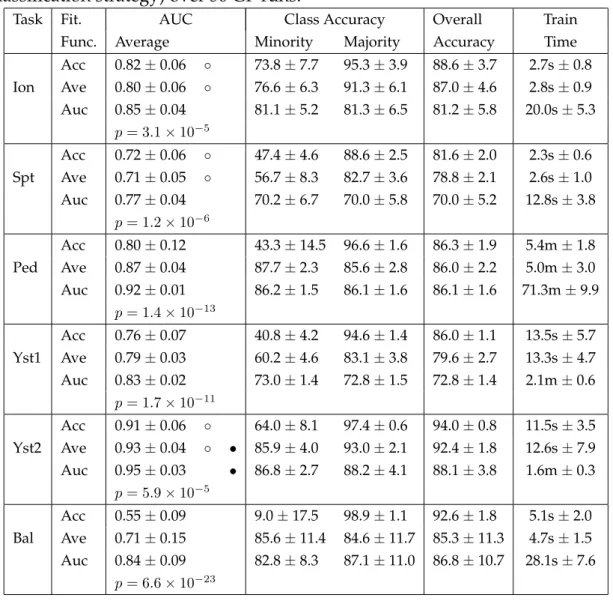
fixed zero-threshold (ZT) and non-static threshold (NST) classifica-tion strategies (statistically significantly better AUC highlighted in bold) over 50 GP runs. . . 68 3.3 Full classification results using the fitness functions (for the ZT

classification strategy) over 50 GP runs. . . 70 4.1 Outcomes of a two-class classification problem. . . 78 4.2 Minority and majority class accuracies of three solutions, and the

correspondingAveM fitness values. . . 79 4.3 Minority and majority class accuracies, and corresponding fitness

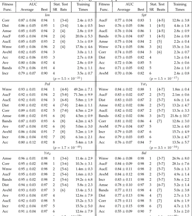
values forAve,AveM andBandsfor four solutions. . . 86 4.4 Full classification results of the GP fitness functions for the tasks.

TheSR denotes the significance rank (s-rank) of a fitness function andbeatsdenotes other s-rank(s) with a (statistically) significantly poorer AUC. . . 94 4.5 Total number and percentage of first, second and third place AUC

positions on a run-by-run basis over 50 GP runs and six tasks (300 total runs). . . 98 4.6 AUC and training time for a single run using Naive Bayes (NB)

and Support Vector Machines (SVM) on the tasks. . . 101 4.7 Average (±standard deviation) AUC for weighted-average fitness

functionAve(Eq. 4.2) on the tasks. TheSRdenotes the significance rank (s-rank) for a weight value andbeats denotes other s-rank(s) with a (statistically) significantly poorer AUC. . . 104

(16)

5.1 Average (± standard deviation) hyperarea of evolved Pareto-approximated fronts, Pareto optimal (PO) front, and training times (seconds ’s’ or minutes ’m’) for the MOGP approaches over 50 runs. The (statistically) significantly better average hyperarea is highlighted in bold, and the higher PO front hyperarea is underlined.122 5.2 The average number of Pareto front solutions that produce distinct

points in objective-space (test set), and the number of Pareto front solutions with different internal models (different AUC) over 50 runs for the MOGP approaches. . . 131 5.3 Average AUC (±standard deviation) of the Pareto front solutions

in four regions of objective-space (from Figure 5.8), and the percent-age of solutions in a given region (over all Pareto front of solutions from 50 runs) for NSGAII and SPEA2 on the tasks. Significantly better AUC between NSGAII and SPEA2 is highlighted in bold. . . 134 6.1 Average (± standard deviation) hyperarea of evolved

Pareto-approximated fronts, and hyperarea of the Pareto-optimal (PO) front for the three MOGP approaches (Baseline, NCL and PFC) over 50 runs. The pairs of hyperarea results in bold or italics denote that these two approaches achieve a statistically significantly better hyperarea than the remaining approach (but not each other). The highest PO front hyperarea from all three approaches is underlined. 155 6.2 Average training times for the three MOGP approaches in seconds

(s) or minutes (m) over 50 runs. . . 156 6.3 Average accuracy (± standard deviation) on the test set and

ensembles size for the Pareto Front ensemble using the majority vote (PF-vote) and fitness-weighted vote (PF-Wvote) over 50 runs. 158 6.4 Average accuracies (± standard deviation) on the test set and

en-sembles sizes using RPF-vote and off-EEL [76] ensemble selection strategies (50 runs). . . 161 6.5 ”Win” pairs between two MOGP approaches (on a run-by-run

basis) over 50 runs for two ensemble combination strategies (PF-Wvote and off-EEL). Total wins (and draws) is the sum of wins (and draws) over all runs and tasks (50 runs×6 tasks). Bold results indicate a statistically significantly better ensemble performance (95% significance level). . . 168

(17)

LIST OF TABLES xv 6.6 ”Win” pairs between the two ensemble combination strategies

(PF-Wvote and off-EEL) for the MOGP approaches (on a run-by-run basis) over 50 runs. Bold results indicate a statistically significantly better ensemble performance (95% significance level) over 50 runs. 170 6.7 Average accuracies (±standard deviation) using canonical

single-objective GP (SGP) on the test set with three fitness functions (Acc,

Aveand Auc) over 50 SGP runs, and a single run of NB and SVM on the tasks. . . 173 6.8 Average accuracies (±standard deviation) on the test set using

PF-Wvote (fitness-weighted majority vote) and off-EEL [76] ensemble selection strategy for the three MOGP approaches (50 runs). These are repeated from Tables 6.3 and 6.4. . . 173 7.1 Ensemble accuracy (± standard deviation) on the test set, and

average ensembles size (minimum ensemble size in parenthesis), for the CSVote and CSLogic approaches to ensemble selection (over 50 runs) when the maximum composite solution tree depth is 2 and 3.196 7.2 Ensemble accuracy (± standard deviation) on the test set and

average ensembles size using off-EEL [76], CSVote and CSLogic (maximum tree depth of 2) for ensemble selection (over 50 runs). . 198 7.3 ”Win” pairs between two MOGP approaches (on a run-by-run

basis) over 50 runs for three ensemble selection strategies (CSVote, CSLogic and off-EEL [76]). A “win” is when one approach dominates the other on a given run. Total wins (and draws) is the sum of wins (and draws) over all runs and tasks (50 runs ×

6 tasks). Bold results indicate a statistically significantly better ensemble performance (95% significance level). . . 199 7.4 Ensemble performances on the training set (TRAIN50) for the

ensem-ble selection approaches (CSVote, CSLogic and off-EEL [76]) over 50 runs. 201 7.5 Average performances of the CSVote approach trained using

VALI-DATION20, and evaluated on TRAIN40 and TEST40 (over 50 runs). . . . 202 7.6 Off-EEL performances using TRAIN40 to train the base classifiers

and VALIDATION20 to select the best ensemble members, and final performance on the unseen test sets TEST40 (over 50 runs). . . 203 B.1 Average AUC (± standard deviation) for fitness functions Corr

and Dist using Ave-based approach for class ordering (W = 2) over 50 GP runs . . . 245

(18)

B.2 Ensemble accuracy (± standard deviation) on the test set using

Y values of 0.25, 0.75 and 1 in the fitness function for the PFC approach (withOff-EEL) over 50 runs. . . 246 B.3 ”Win” pairs when the current PFC approach (PFC0.5) is compared

to otherY values in the fitness function (PFCY) withOff-EEL (on a run-by-run basis) over 50 runs. Bold results indicate a statistically significantly better ensemble performance (95% significance level) over 50 runs. . . 247

(19)

List of Figures

2.1 An ROC curve where operating points A, B and C represent the classifier’s performance at three different decision thresholds. . . . 17 2.2 Example of an encoded 8 bit binary chromosome (individual) in GA. 18 2.3 Evolutionary search in GP. . . 22 2.4 Crossover operator in GP. . . 24 2.5 Mutation operator in GP. . . 25 2.6 (a) Different sets of non-dominated solutions returned from four

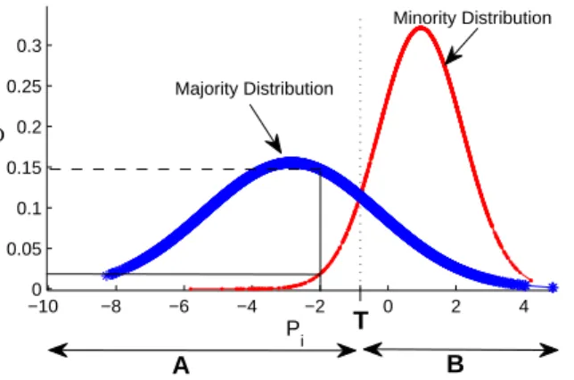
EMO runs; and (b) the median attainment surface with respect to 50 EMO runs. . . 32 2.7 Classification strategy in GP. . . 33 3.1 Distributions of minority and majority class outputs for two GP

solutions (output values along the horizontal axis) and target class regions. . . 57 3.2 Distributions of class outputs for a GP solution andφvalues of the

outputsPc,i for the two classes. . . 60 3.3 (a) Shaded area is the trapezoid fitted under two points on an ROC

curve wherewis the width, andhandh′are heights of the trapezoid. 63 3.4 (a) Numeric outputs of a GP solution when it is evaluated on the

input instances, where+and - denote the positive (minority) class and negative (majority) class outputs, respectively, andTi and Tj are two different class thresholds; (b) an ROC curve with two points. . . 64

(20)

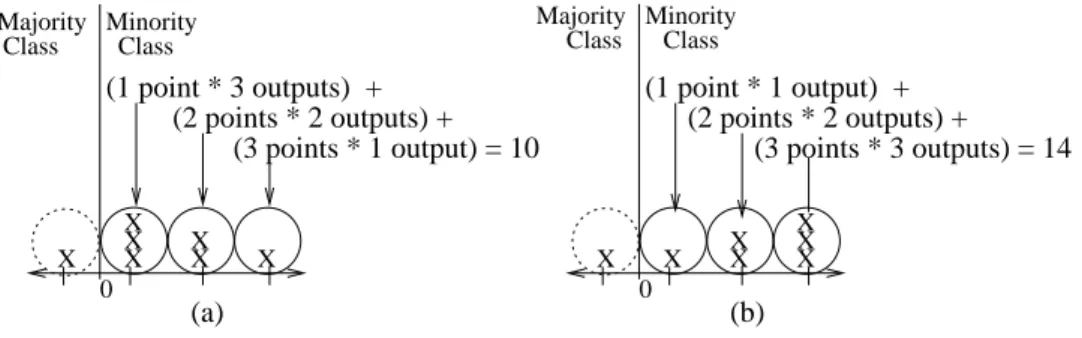
4.1 Genetic program outputs for two classifiers; X denotes the solu-tion outputs for seven (minority class) instances where equivalent

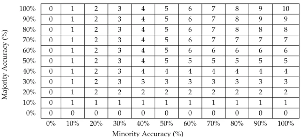
Xvalues are stacked above each other. Solid circle shows correctly predicted clusters of outputs and dotted circle shows incorrect clusters. Solution(b)is better as it earns 14 rewards while(a)only earns 10, as (b) has more outputs that lie further away from the class boundary (0). . . 84 4.2 Regions of fitness bands (for fitness function Bands) where the

objective-space is divided into a 10×10 grid and each grid square represent the fitness value for the minority and majority class accuracy of a solution). . . 85 4.3 Confidence intervals of the AUC for the different fitness

func-tions for the Ion task. In (a), the interval for Acc is statistically significantly poorer than Dist and Corr. In (b), the confidence intervals are labelled with their s-ranks where the legend shows significantly better s-ranks. . . 91 4.4 Typical ROC Curves (test set) for the GP fitness functions on four

tasks. The true positive (TP) rate is the minority class accuracy, and false positive (FP) rate is 1−the majority class accuracy. The axis scopes are different in each figure. . . 100 4.5 Minority and majority class accuracies (on the test sets) for

weight-ing coefficientW in fitness functionW ave(axis scopes are different in each figure). . . 106 4.6 Evolved GP classifier with a high AUC (0.98) on Bal. . . 107 4.7 Evolved GP classifier with an above average AUC (0.92) on Bal. . . 108 4.8 Evolved GP classifier with a typical AUC of 0.85 on Bal. . . 109 4.9 Smallest evolved GP classifier with an AUC of 0.84 on Bal. . . 110 5.1 Pareto-based fitness values for NSGAII and SPEA2 where filled

points are dominated solutions and filled points are non-dominated solutions. . . 118 5.2 The “crowding” distance used in MOGP. . . 118

(21)

LIST OF FIGURES xix 5.3 Classification performance of evolved solutions using two MOGP

approaches (NSGAII and SPEA2), and canonical SGP using fitness functions W ave. In Ion, Ped and Yst2 ( top row), the average

hyperarea for SPEA2 is statistically better than NSGAII. There is no significant difference in hyperarea for the remaining tasks (bottom row). . . 125 5.4 Accuracy of all Pareto front solutions evolved over 50 runs for the

MOGP approaches on three tasks (Ion, Ped and Yst2). Circle size is

proportional to frequency. . . 127 5.5 Accuracy of all Pareto front solutions evolved over 50 runs (Ped

task) where circle size is proportional to frequency. . . 128 5.6 Output values denoted by+and − for the positive and negative

class, respectively, for two solutions (p1 and p2). In (a), p1 and p2

have the same accuracy on the two classes relative to zero as the class threshold; while in (b),p1andp2have different accuracy rates

on the two classes relative to class thresholdi. . . 130 5.7 AUC of all Pareto front solutions evolved over 50 MOGP runs for

NSGAII (top) and SPEA2 (bottom) on two tasks (Ped and Yst1).

Each vertical bar represents a Pareto front solution (on the two objectives) and the heights of the vertical bars represent the AUC. . 132 5.8 The regions of objective-space. . . 133 6.1 (a) The (processed) outputs for three solutions and the ensemble

output (E) on the five inputs (incorrect predictions are underlined assuming that the target class label is 1). (b) The three steps to calculate the NCL for solution a3 where final NCL value fora3 is

0.15P_Mstep 3_×_N c = 2.25 3×5 . . . 148 6.2 Pairwise PFC comparisons between three solutions (a1, a2 anda3)

on five inputs (in the same class). . . 151 6.3 MOGP ensemble performances on the minority and majority class

(test set) using PF-vote over generations for Baseline and PFC. . . . 159 6.4 MOGP ensemble accuracies (on a run-by-run basis) and median

attainment surface (“average” front performance) for Baseline and PFC approaches with off-EEL for 50 runs. . . 165 6.5 Evolved MOGP classifier with 100% accuracy on training and test

set for Bal. . . 175 6.6 An evolved MOGP ensemble program for Bal. . . 177

(22)

6.7 (a) Overall structure of two GP trees (for Bal) whererepresents a sub-tree (omitted) and the dashed rectangles (around a given sub-tree) show where in the overall structure the seven differences occur; and (b) sub-trees in the second GP tree that are different from Figure 6.6. . . 177 6.8 A smaller evolved GP tree (for the Bal task). . . 178 7.1 Overview of the process for ensemble selection using composite

so-lutions and off-EEL [76] for a given set of base classifiers (evolved Pareto front from a MOGP run). . . 186 7.2 Combining a subset of Pareto front solutions (from a given MOGP

run) into a single composite solution. . . 187 7.3 Raw (real-valued) output values and predicted class labels for five

Pareto front solutionspi (when evaluated on a given input). Raw outputs are mapped to class labels using zero as the class threshold. 188 7.4 Composite voting solution (CSVote) and evaluation of this CSVote

tree using terminal node values from Figure 7.3 (tree output is the class label 1 denoting the minority class). . . 190 7.5 Composite logic solution (CSLogic) and evaluation of this CSLogic

tree using terminal node values from Figure 7.3 (tree output is the class label 1 denoting the minority class). . . 191 7.6 Fully formed composite trees of depth 2 and 3. . . 193 A.1 (a) Example pedestrian (left two) and non-pedestrian image (right

two), and (b) local image regions for extracting pixel statistical features. . . 242

(23)

Chapter 1 Introduction

Classification is the act of placing an object into a set of classes or categories based on the object’s properties or features [68]. Given the abundance of real-world information now being captured and stored digitally, systems that can automatically search for and identify valid and useful patterns in data for classification, with as little human intervention as possible, are fast becoming highly desirable.

However, creating intelligent learning systems that perform classification reliably and with a sufficient level of accuracy, is difficult. Genetic Programming (GP) is a machine learning and search technique which has been successful in building reliable classifiers to solve classification problems [104][62][176]. GP is an evolutionary learning algorithm which uses the principles of Darwinian evolution and natural selection to evolve computer programs to solve a particular problem. In GP, programs representing different solutions to a problem are combined with other programs to create new, hopefully better, programs over a number of generations, until an good solution is evolved [104].

In many real-world applications, such as fraud detection [157][67][159], med-ical diagnosis [80][88], bioinformatics [132], or fault diagnostics [142], it is not uncommon to have a disproportionate number of training examples in one class compared to the other class(es). This is known asclass imbalanceand occurs when at least one class is represented by only a small number of examples (called the

minority class) while the other class(es) make up the rest (called themajority class) [38].

(24)

1.1 Motivation

Recent work in the machine learning community has highlighted that the class imbalance problem represents a major obstacle in classifier learning [38][172][93]. This is due to the performancebias that can occur when an uneven distribution of class examples is used in the learning process. Here learnt classifiers can exhibit high accuracy on the majority class(es) but poor accuracy on the important minority class(es) [141][57][173]. As the minority class usually represents the main class-of-interest in most real-world classification problems, accurately clas-sifying examples from this class isat leastas important as, and in some scenarios more important than, accurately classifying examples from the majority class [67][159][142].

Addressing this learning bias to correctly classify examples from both the minority and the majority classes equally well has become an important area of research [38]. Work in this area tends to focus on three main aspects. The first involves sampling [157][12][11], or transforming [173][85], the original un-balanced data set to create artificially un-balanced classes for the training process (so-called “external” approaches). The second aspect involves various forms of cost adjustment within the learning algorithm to utilise the original unbalanced data “as is” in the training process; these are known as “internal” approaches as the learning algorithm itself is adapted to account for the uneven distribution of class examples [27][60][34]. The third aspect uses ensemble learning where multiple trained classifiers are aggregated together to determine the final prediction [159][164][123]. Ensemble learning uses aspects from both external and internal approaches to train the individual base classifiers. In bagging and boosting techniques, the training data is partitioned into smaller, balanced subsets of class examples using sampling techniques [123][118][170][37]; while in other ensemble learning approaches, a diversity measure is used in the fitness function to encourage cooperation between the base classifiers [119][36][3].

While external approaches can be effective, they have major disadvantages. Sampling can add a computationally expensive overhead to the training process as, in most cases, this must be applied repeatedly for good coverage. These techniques can also requirea prioriexpert knowledge about the data [157]. More importantly, sampling techniques can suffer frompoor generalisationas potentially useful learning examples can be excluded from the learning process, and the learnt models do not capture the underlying rarities that occur in unbalanced data sets (as the training set is first artificially re-balanced).

(25)

1.1. MOTIVATION 3 Due to these limitations, machine learning practitioners have recently focused on internal approaches using cost adjustment in the learning algorithm. Common approaches include using fixed misclassification costs for minority and majority class examples [88][142], or developing improved training criteria that are sensi-tive to the unbalanced class distributions (unlike the traditional overall accuracy measure). Improved training criteria for class imbalance includes the average classification accuracy of the minority and majority class [107][139][5][116], and the Area under the Receiver Operating Characteristics (ROC) curve (also known as the AUC) [27][84][149][90]. ROC curves are a useful technique to capture the performance trade-off between the minority and majority class accuracies in the learnt models across varying classification thresholds. In GP specifically, much work has focused on adapting the fitness function to reward solutions that are accurate on both the minority and the majority classes [141][57].

While these internal cost-adjustment based approaches can substantially improve minority class accuracy, there are three main limitations. Firstly, misclassification costs for incorrect class predictions must usually be determined

a priori, where these costs can be problem-specific and require a lengthy trial-and-error process to configure [157][88][142]. Secondly, improved performance metrics in the fitness function (such as the AUC) can substantially increase training times due to the computational overhead required to calculate these measures, particularly on large data sets [34][179]. Finally, new fitness functions can be hand-crafted to suit a particular classification problem, requiringa priori

expert knowledge about the problem domain [157][60]. In this area there is a need to develop new performance measures in the fitness function which can evolve solutions with good classification ability on both classes, without incurring a substantial increase in training times, and which are problem-independent.

Evolutionary multi-objective optimisation (EMO) is a fast-growing area of research which offers a promising solution to learning with multiple objectives that are in conflict. Unlike single-predictor classifier induction techniques where the fittest individual is returned from the training process, in EMO a set (or

Pareto front) of solutions is evolved to capture the performance trade-off between the different objectives. EMO accomplishes this by treating the objectives independently in the learning process using the notion of Pareto Dominance in fitness. Pareto Dominance establishes a ranking of the individuals in the population according to how well they perform on all the objective with respect to each other [42][78].

(26)

model regularization, ROC optimisation and ensemble learning. The first two of these problem domains typically involves classification tasks where the class distributions are assumed to be balanced. In model regularization, the (overall) accuracy is traded-off against the complexity or size of the learnt models [70][92][50]; while in ROC optimisation, the true positive and false positive rates are traded-off each against other [162][108][65].

However, in EMO-based ensemble learning for classification with unbalanced data, most approaches use neural networks, decision trees or Naive Bayes as the base classifiers [123][118][170][37], and rely on sampling techniques to re-balance the training data during fitness evaluation [159][123][170][168]. This means that most of these works assume that the classes are balanced before the diversity between the solutions are calculated. A GP-based multi-objective GP approach where the accuracy of the minority and majority classes are traded-off against each other in the learning process for cost-adjustment, thereby allowing the original unbalanced training data to be used “as is” in the learning process (without sampling), has not previously been explored. In addition, very few works in this area investigate how to adapt the diversity measures in the fitness function to account for skewed class distributions [168].

1.2 Research goals

To address these limitations, the overall goal of this thesis is to develop new internal cost-adjustment techniques in GP for binary classification problems with unbalanced data. To achieve this goal, two GP approaches are proposed, each with a specific set of research objectives:

1. Develop new improved fitness functions in canonical single-objective (“single-predictor”) GP using the ROC curves of the evolved classifiers to represent the performance trade-off between the minority and the majority class accuracies.

a) Develop a suitable GP approach and classification strategy for binary classification tasks with unbalanced data.

b) Develop new, improved performance measures in the fitness function which account for both the minority and the majority class accuracies in the evolved classifiers.

(27)

1.3. MAJOR CONTRIBUTIONS 5 2. Develop a new GP-based multi-objective approach to representing the

per-formance trade-off between the minority and the majority class accuracies. a) Develop a multi-objective GP approach to evolving a Pareto front of

genetic program classifiers along the minority and majority class trade-off frontier using Pareto dominance in the fitness function.

b) Develop an ensemble learning approach to combining Pareto front classifiers using fitness functions that promote diversity between in-dividuals equally on both classes.

c) Develop new cooperative classification strategies in the ensemble using small highly-cooperative groups of individuals.

Focusing on internal cost adjustment using the fitness function allows the unbalanced data to be used “as is” in the learning process, requiring no external data-balancing techniques to artificially re-balance the input data prior to the learning process. This thesis focuses on internal methods due to three important considerations.

• All learning data is assumed to be useful and shouldnotbe excluded from the learning process (external data-balancing techniques can exclude useful learning instances in training).

• The GP approaches should be problem-independent and not require anya priori data-specific or expert knowledge about the input data. This means that the new methods should work well when the unbalanced data sets are used directly (or “as is”) in the GP learning process, requiring no prior pre-processing or transformations for data-balancing.

• Using the unbalanced learning data directly in the training process allows us to concentrate on the properties established by the new cost adjustment techniques in the GP algorithm. Thus, any improvements can be attributed to these properties and not a given sampling policy.

1.3 Major Contributions

This thesis makes the following major contributions.

1. The thesis shows how to address binary classification problems with unbal-anced data using GP, with particular focus on cost-adjustment within GP

(28)

rather than the traditional data-balancing techniques. In the GP approach, this thesis finds that there is no major differences in performance using the traditional (static) classification strategy and a dynamic (non-static) classification strategy on these binary class imbalance tasks. This shows that GP can sufficiently tweak the mathematical expressions representing the classifiers to “shift” its outputs relative to the fixed class boundary. This is not the case for multiple-class tasks according the the current literature which shows that the dynamic strategy outperforms the traditional (static) classification strategy. Rather, this thesis shows that the configuration of the fitness function in GP is more important for evolving well-performing classifiers. These results have been published in [16].

2. This thesis proposes several new measures in the fitness function in GP to perform cost adjustment between the minority and the majority class accuracies, allowing the unbalanced data sets to be used directly in the learning process without first re-balancing the data (via sampling). By treating these two objectives as equally important in the learning process, these new measures in GP find classifiers with good classification ability on both classes (high AUC), which outperform Naive Bayes (NB) and Support Vector Machines (SVM) on tasks with very high levels of class imbalance. On these tasks, both NB and SVM methods show very biased classification results. These results have been published in [13][14][17].

3. This thesis proposes a multi-objective GP (MOGP) approach where the accuracies of the minority and the majority classes are traded-off against each other in the learning process. The novelty of this approach is that a Pareto-based fitness function is used to the treat the unbalanced classes independently (i.e. as separate objectives) for cost adjustment when the unbalanced data is used directly in the learning process. This allows multiple trade-off solutions to be evolved in a single optimisation run, leaving the final choice for the decision-maker; whereas canonical (single-objective) GP requires a much longer time to get a reasonable front as the objective preference is specified a priori. MOGP using the SPEA2 [188] Pareto dominance algorithm is found to perform as well as, and in some cases better than, multiple runs of canonical single-objective GP; while MOGP using the NSGAII [53] algorithm cannot achieve this to a sufficient level of accuracy. These results have been published in [15][20][21].

(29)

1.4. ORGANISATION OF THESIS 7 diversity between individuals and combine Pareto front classifiers into an ensemble where members vote on the class label. Unlike traditional ensem-ble learning approaches (where the unbalanced data is first re-balanced via sampling), the measures are adapted to calculate diversityseparatelyfor the two classes (to account for the unequal classes); otherwise, the diversity measures risk being biased toward the majority class. When diverse Pareto front solutions work together to classify the data instances, the evolved ensembles, in particular MOGP with the pairwise failure crediting diversity measure, perform better than their individual members, due to good cooperation between members on the tasks. These results have been published in [22][19].

5. This thesis shows how GP can be used for ensemble selection (and pruning) to quickly find diverse subsets of Pareto front individuals that cooperate well together in the ensemble. To avoid “fine tuning” a large weight vector (as used in traditional ensemble selection), the new approach evolves composite GP solutions to represent the (final) ensemble, by combining multiple Pareto front individuals into a single composite solution. The main novelties of the new approach include using selection pressure in the evolution to find small groups of diverse members for the ensemble (by imposing a size constraint on the GP solutions), and different function sets to manipulate the outputs of the individual members (to control the final ensemble classification decision). The GP composite solutions use fewer individuals in the ensemble to produce ensemble results that are as good as, and in some cases better than, an existing approach to ensemble selection (Off-EEL [76]), particularly on tasks with very high levels of class imbalance. These results have been partially published in [18].

1.4 Organisation of Thesis

The remainder of this thesis is organised as follows. Chapter 2 carries out a literature review; the five main contribution chapters, Chapters 3–7, address each of the five sub-goals in this thesis; and Chapter 8 concludes this thesis.

The literature review in Chapter 2 is split into two parts: background and related work. The background covers the fundamental concepts in evolution-ary computation focusing on GP, ensemble learning, and evolutionevolution-ary multi-objective optimisation. The related work discusses the recent advances in GP for

(30)

classification, class imbalance learning with particular focus on GP and ensemble-based approaches, and EMO for classification. The related work also discusses the limitations of the current approaches and the challenges that the thesis attempts to address.

Chapter 3 proposes the GP framework for classification, with particular emphasis on the classification strategy used in the evolution, and evaluates three major current approaches in the fitness function to highlight the advantages and limitations of each approach and why they need to be improved. This evaluation contrasts the AUC, the overall accuracy, and individual class accuracies of the evolved GP classifiers to justify why the AUC is a better performance measure in these class imbalance scenarios, rather than the traditional overall accuracy.

Chapter 4 develops several new performance measures in the fitness function to address the limitations highlighted in Chapter 3. Focusing on the AUC of the evolved classifiers, the new methods are compared to several current approaches in the the fitness function from the literature (including those from Chapter 3), and two other popular machine learning algorithms (Naive Bayes and Support Vector Machines). These fitness functions are ranked using a new measure designed to capture the statistical significance relationships between the new fitness functions on the unbalanced data sets. Several evolved GP classifiers are analysed to gain a better understanding of how GP learns to solve a given problem.

Chapter 5 develops the multi-objective GP (MOGP) approach using the accuracies of the minority and the majority classes as the two competing learning objectives. Particular emphasis is placed on how to represent Pareto dominance in the fitness function, where two popular dominance-based ranking algorithms from the literature (SPEA2 [188] and NSGAII [53]) are compared in fitness. The performance of the evolved Pareto-approximated fronts and the AUC of the Pareto front solutions, are compared to the single-objective GP (SGP) methods (from Chapter 4) to highlight the major differences between these methods.

Chapter 6 develops an ensemble learning approach to combining the evolved set of Pareto front classifiers (from the MOGP approach in the previous chapter) into an ensemble where members vote on the class label. Two ensemble-diversity measures are developed and incorporated in the fitness function in MOGP to promote cooperation between solutions, and the diversity-based ensembles are compared to an MOGP approach using no explicit ensemble-diversity measure in fitness. The ensembles are evaluated using two combination strategies to combine the outputs of the individual members, and two selection strategies to

(31)

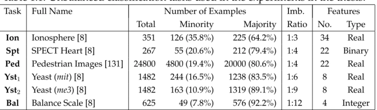
1.5. BENCHMARK TASKS WITH UNBALANCED DATA 9 Table 1.1: Unbalanced classification tasks used in the experiments in the thesis.

Task Full Name Number of Examples Imb. Features Total Minority Majority Ratio No. Type

Ion Ionosphere [8] 351 126 (35.8%) 225 (64.2%) 1:3 34 Real

Spt SPECT Heart [8] 267 55 (20.6%) 212 (79.4%) 1:4 22 Binary

Ped Pedestrian Images [131] 24800 4800 (19.4%) 20000 (80.6%) 1:4 22 Real

Yst1 Yeast (mit) [8] 1482 244 (16.5%) 1238 (83.5%) 1:6 8 Real Yst2 Yeast (me3) [8] 1482 163 (10.9%) 1319 (89.1%) 1:9 8 Real Bal Balance Scale [8] 625 49 (7.8%) 576 (92.2%) 1:12 4 Integer

only select accurate and diverse individuals for the ensemble. Several evolved MOGP classifiers are also analysed and compared to canonical SGP classifiers.

Chapter 7 develops a new GP approach to ensemble selection to quickly find groups of diverse Pareto front individuals that cooperate well together in the ensemble, improving ensemble performances from the previous chapter. Composite solutions are developed to represent the (pruned) ensembles; these amalgamate multiple Pareto front individuals into a single genetic program. Two types of composite solutions are developed, composite voting solutions and composite logical solutions, and these are compared to the ensemble selection strategies from the previous chapter.

Chapter 8 concludes this thesis by summarising the main conclusions and research objectives achieved in the individual chapters, and provides further discussions on more general topics covered in the whole thesis, and areas of future work.

1.5 Benchmark Tasks with Unbalanced Data

Throughout this thesis, the proposed GP methods are evaluated on six real-world benchmark classification tasks with unbalanced data from theUCI Repository of Machine Learning Databases[8], and the Intelligent Systems Lab at the University of Amsterdam [131]. These tasks are summarised in Table 1.1; for a detailed description of each task, please refer to Appendix A.

In each task, half of the examples in each class are randomly chosen for the

trainingand the testsets. This ensures that both training and test sets preserve the same class imbalance ratio as the original data set. While it is possible that the class distributions in the training set and test set can be different, this thesis only considers tasks with similar distributions in both sets for comparison and generalisation purposes.

(32)

These benchmark data sets are carefully selected to encompass a varied collection of problem domains to ensure that the evaluation of the different GP approaches is not problem-specific. These problems have varying levels of class imbalance (minority class ranges between 7% and 35% of total examples), and complexity where some tasks are more easily-separable than others. The training and test sets also range from being well-represented (e.g. Ped has approximately 12000 instances), to sparsely-represented (e.g. Spt only has 27 instances from the minority class). These tasks also range between high and low dimensionality (e.g. Ion has 34 features while Bal only has 4), and use different features types (binary, integer and real features). Therefore, these data sets are expected to represent class imbalance problems of varying difficulty, dimensionality, size and (feature) types reasonably well. None of these data sets contains missing attributes — this is an interesting topic but beyond the scope of this thesis.

(33)

Chapter 2 Literature Review

This chapter provides the background and related work for this thesis. The first four sections of this chapter discuss the background material, including the following four topics: machine learning and classification, evolutionary compu-tation, genetic programming (GP), and evolutionary multi-objective optimisation (EMO). The last two sections of this chapter discuss the related work which is split into two main categories. The first outlines the related work in GP and EMO for classification with balanced data, while the second outlines the related work in the wider machine learning community (including GP) for classification with unbalanced data.

2.1 Machine Learning

Machine learning is a broad and rapidly developing area of research [114][33][59]. Different artificial intelligence experts in this field vary in their definitions of what exactly constitutes machine learning but most agree that the central idea involves computer programs which learn to solve problems without explicitly being programmed or told how to do so [97][7][24][150].

Traditionally, learning methods have been split into three main strategies: su-pervised, unsupervised and reinforcement learning [24][150]. Supervisedlearning is learning with labeled class examples or instances. In supervised learning, the actions or desired outputs for a problem are known in advance, and the learning system tries to find rules or a function to map its outputs to the desired (or target) outputs. Unsupervised learning is learning without labeled class examples. In unsupervised learning, there are no correct answers for the learner to explicitly learn from. Instead, the learner must explore underlying structures or similarities in the data to find useful patterns such as clusters. In reinforcement learning,

(34)

the learner receives feedback based on its actions (outputs) in terms of rewards or punishments but unlike supervised learning, the desired outputs are not explicitly provided.

2.1.1 Classification

Classification is a supervised machine learning task where the system learns from a set of labeled input examples or instances. Given a set of attributes or features and their corresponding class labels, classification involves learning a model to correctly predict the class membership of each attribute [129][32].

Common to supervised learning problems are the concepts oftrainingandtest

sets. A training set is a collection of input patterns from which classification rules are induced. A test set is a similar collection of input patterns, except that these are not used during the learning process and remain unseen while learning the rules. The purpose of the test set is to evaluate the performance of the learnt rules on unseen instances of the problem. This is important as it verifies that the learnt rules are notover-fitted to the training set. In supervised learning, the procedure for learning is two-fold: discover/learn the rules or a function for the input-output mappings using the training set, and apply these rules or functions to the test set to determine how well the learnt concepts perform (orgeneralise) on unseen problem instances.

This thesis focuses on supervised learning. In this area, there are many different learning paradigms, some include the following (the four paradigms discussed below are used in the experimental results throughout the thesis).

Bayesian Classifiers

Bayesian classifiers use a probabilistic approach to classification based on Bayesian probability principles. Naive Bayes (NB) is a simple but popular Bayesian classifier which uses Bayes’ theorem to compute unknown probability estimates (i.e. the class of an unseen instance) from known ones (i.e. features of known instances) [129]. NB is remarkably effective in practice and can show competitive results compared to other more-complex learning paradigms [129][178]. However, NB makes strong (naive) assumptions about the conditional independence of the features where the presence (or absence) of a feature is as-sumed to be completely unrelated to the presence (or absence) of another feature. Bayesian belief networks [94] address this issue of conditional independence by representing dependencies between features as a directed graph.

(35)

2.1. MACHINE LEARNING 13

Statistical Paradigms

Support Vector Machines (SVMs) [167] is a statistical supervised learning algo-rithm. SVMs construct a number ofhyperplanesin the (high-dimensional) feature-space that aim to separate the input instances from the two classes, and then try to maximise the distance between the decision hyperplanes and the input instances from both classes (this distance is called the margin). The original SVM algorithm was a linear classifier where the input instances are assigned a class label depending on which side of a decision hyperplane they lie on [167]. However, the current version useskernel functionsto construct non-linear decision surfaces [44].

Genetic Paradigms

Genetic paradigms comprise of a wide range of nature-inspired computational methodologies that incorporate the modern principles of Darwinian evolution and natural selection into machine learning. Popular genetic paradigms include genetic algorithms [86] and genetic programming [104] which is also the focus of this thesis. These paradigms and other evolutionary computational methodolo-gies are discussed in more detail in the next section.

Ensemble Paradigms

Ensemble methods combine together multiple learnt models to obtain better predictive performance than could be obtained from any of the single constituent models [31][129]. In an ensemble of classifiers, amajority voteis typically used to combine the outputs of the individual members: for a given input, each member votes on the output (e.g. predicted class label), and the class label with most votes is chosen as the ensemble output. Ensemble methods can be used with base learners from different learning paradigms, provided that the base classifiers are accurate and diverse with respect to their outputs [54][31]. Diverse ensemble members should not make the same errors on the same inputs, otherwise the ensemble will risk misclassifying the same inputs together each time.

Other Paradigms

In addition to the above-mentioned learning paradigms, there are also many other learning paradigms. Three important categories include the following (the

(36)

three paradigms discussed below are not used in this thesis but are included to give the reader a better idea of this field).

Connectionist Paradigms. These include artificial neural networks (ANNs) [23] which are computational models inspired by biological neural networks. An ANN consists of an interconnected group of artificial neurons (called nodes), where information (usually numeric) travels through nodes in different layers of the network. In classification, ANNs can model complex relationships between inputs (e.g. features) and outputs (class membership) to find patterns in data. However, ANNs are typically “black-box” learners as end-users cannot easily interpret the learned concept to understand how an ANN has learned to solve a problem.

Case-Based Reasoning. These include the nearest neighbour algorithm [45] which classifies an unseen instance as the same class of the closest training instance in feature-space. These learning paradigms arelazy in that they do not attempt to learn or generalise a classification model using the training data.

Induction Based Reasoning. These include decision tree algorithms which seek to split features that best separate the input instances from the training set [129]. Decision trees classify instances by traversing a tree in top-down manner, starting at the root node and ending at a leaf node which represents the class label. Decision trees are easy to interpret as they represent if-then classification rules; popular algorithms to build decision tree includeID3[147] andC4.5[148].

2.1.2 Class Imbalance Learning

In many real-world applications, it is not uncommon to have disproportionate numbers of learning instances for one class compared to the other class(es). In classification with unbalanced data (also known as the class imbalance problem), at least one class is represented by only a small number of examples (called theminority class) while the other class(es) make up the rest (called the majority class). Research in the machine learning community has highlighted that using unbalanced data in the learning process can leave the learnt classifier with a performance bias, that is, classifiers exhibit high accuracy on the majority class(es) but poor accuracy on the minority class(es) [38][93][172][130][69]. Addressing this learning bias to find classifiers with good accuracy on both the minority and majority class is an important area of research and the focus of this thesis.

(37)

2.1. MACHINE LEARNING 15 The following is list of real-world problems affected by class imbalance.

• In fraud detectiontasks such as network intrusion detection [157], telephone fraud [67], and credit card fraud [159], fraudulent transactions are relatively small compared to the vast majority of normal transactions.

• In medical diagnosis of rare medical conditions, the majority of patients are healthy and only a small minority will be diseased [80][88][41].

• Inbio-informaticstasks such as protein classification, the target protein class is small compared to non-target (normal) proteins [132].

• In financial risk modeling such as loan approval or insurance risk modeling, high-risk applicants are rare in comparison to normal loan or insurance applicants [143].

• In some data miningtasks such as direct marketing, negative responses are typically small compared to positive responses [117]; or inchurnprediction [179], relatively few customers switch subscriptions compared to those who do not.

• Inimage recognitionor object detection tasks such as target [89], face [161] or pedestrian [162] detection, the important objects-of-interest are typically in the minority class compared to non-objects (background).

• In fault diagnostics such as industrial defect detection [85] or network trou-bleshooting [142], faulty instances are typically rare compared to normal instances.

2.1.3 Evaluating Classifier Performance

The traditional measure to evaluate the goodness or success of a learnt classifier uses the overall classification accuracy (or overall error rate) on the learning instances [129]. The overall accuracy is the number of inputs correctly labeled by the classifier as a proportion of the total number of inputs seen by the classifier. Using the four different outcomes for binary classification shown in Table 2.1, the overall accuracy can be expressed by the equation below. In Table 2.1, assume that the minority class is thepositiveclass.

accuracy= T P+T N

(38)

Table 2.1: Outcomes of a two-class classification problem.

PredictedPositive Class PredictedNegative Class

ActualPositive Class True Positive (TP) False Negative (FN)

ActualNegative Class False Positive (FP) True Negative (TN)

However, the overall accuracy is known to be unsuitable for classification with unbalanced data [93][130][172][69]. This is because this measure considers all learning instances as equally important and does not take into account that the number of learning instances in the minority class can be much smaller than in the majority class. Abiased classifier which has very poor accuracy on the minority class but high majority class accuracy, can also have a high overall accuracy due to the influence of majority class learning instances.

Measuring the individual classification accuracy of the minority and majority class separately such as the true positive (TP) rate and true negative (TN) rate, respectively, as shown below, can avoid this learning bias when evaluating classifier performance in class imbalance scenarios.

TP rate= T P

T P+F N and TN rate= T N

T N+F P (2.2)

The TP and TN rates are similar to the sensitivity and specificity, or precision and recall, as used in the context of other tasks (such as information retrieval) [178]. These measures all accomplish the same goal in classification, that is, categorising the type of error made by a classifier. Precision and recall are defined as:

Precision= T P

T P+F P and Recall= T P T P+F N Sensitivity and specificity are defined as:

Sensitivity=Recall and Specificity= T N T N+F P

The TP and TN rates are usually in conflict with each other where an improvement in one class (e.g. TP rate) produces a trade-off in the other (e.g. TN rate).

ROC Curves

Receiver Operating Characteristic (ROC) curves were originally used in signal detection theory to characterize the trade-off between hit rate and false alarm rate over a noisy channel [84]. This is now widely used in machine learn-ing to evaluate a classifier’s performance across varylearn-ing decision thresholds

(39)

2.1. MACHINE LEARNING 17

C

1 TP

0 _FP

1 B

A

Figure 2.1: An ROC curve where operating points A, B and C represent the classifier’s performance at three different decision thresholds.

[111][149][130][172]. On a ROC curve, the TP rate is plotted against the false positive (FP) rate, as seen in Figure 2.1, where each operating point (e.g. A, B and C in Figure 2.1) represents the TP and FP rates at a given decision threshold. In the context of binary classification, assuming the minority class is the positive class, the TP rate is the minority class accuracy, and FP rate is 1-minority class accuracy (or 1-TN rate).

The lower-left corner on an ROC curve (when TP and FP rates are 0) represents the decision threshold where all inputs are classified as belonging to thenegative

class. The upper-right corner (when TP and FP rates are 1) is the decision threshold where all inputs are classified as belonging to thepositiveclass. Perfect classification accuracy (all inputs correctly classified) is achieved when the TP rate is 1 and FP rate is 0 (top-left corner). The linex=yrepresents the strategy of randomly guessing the class label for a given input.

The area under an ROC curve (AUC) summarises theclassification ability of a classifier across different decision thresholds, and represents theprobability that an input from the positive class is correctly predicted by a given classifier [27][84]. AUC values range between 0 and 1 where the higher the value, the better the performance. Unlike the overall classification accuracy, the AUC is known to be invariant to unbalanced data and is not influenced by the larger majority class in class imbalance scenarios [173][93][130][172].

The AUC is typically approximated using the trapezoidal technique [84] where the AUC is calculated as the sum of the areas of individual trapezoids fitted under each pair of points of the ROC curve.

(40)

2.2 Evolutionary Computation

Evolutionary computation (EC) is a sub-field of artificial intelligence that com-prises of nature-inspired computational methodologies. The two main categories in the area include evolutionary algorithms and swarm intelligence [97][99].

2.2.1 Evolutionary Algorithms

Evolutionary Algorithms (EAs) are a class of algorithms that incorporate the modern principles of biological evolution and Darwinian theories of natural selection of species into machine learning. These theories assert that only the fittest organisms will survive to reproduce while the less fit die off. As the offspring of fit parents will have similar or the same genetic code as their parents, the new generation of organisms is expected to be fitter, or at least as fit, as the current generation. An advantage of EA’s is the ability to navigate through “worse” areas of the search-space in order to avoid becoming stuck in a local

optima.

In EAs, an individual (or member of the population) represents a potential solution to a given problem, and these individuals are evolved (or improved) over generations using genetic operators. Genetic operators are mechanisms inspired by biological evolution such as crossover, mutation or reproduction, to create and improve individuals in the population. A fitness function determines the “goodness” of an individual, that is, how well an individual solves a given problem. Members of the population are selected for recombination (using the genetic operators) depending on their fitness. The goal in EAs, similar to natural selection, is to have some useful part of an individual’s genetic code propagated down generations until an individual with good fitness is evolved.

The main EA techniques include the following.

Genetic Algorithms

Genetic Algorithms (GAs) are one of the earliest representations of an artificial evolutionary learning system [86][79]. In GA, individuals or chromosomes are typically encoded as fixed-length bit strings where each element in this string is called agene, as shown in Figure 2.2.

1 1 0 0 1 0 0 1