On the online classification of data streams using weak estimators

(1)

On the Online Classification of Data Streams

Using Weak Estimators

Hanane Tavasoli1

, B. John Oommen1⋆_{, and Anis Yazidi}2 1

Department of Computer Science, Oslo and Akershus University College of Applied Sciences, Norway

2

School of Computer Science, Carleton University, Ottawa, Canada

Abstract. In this paper, we propose a novelonline classifier for com-plex data streams which are generated from non-stationary stochastic properties. Instead of using a single training model and counters to keep important data statistics, the introduced online classifier scheme provides a real-time self-adjusting learning model. The learning model utilizes the multiplication-based update algorithm of the Stochastic Learning Weak Estimator (SLWE) at each time instant as a new labeled instance arrives. In this way, the data statistics are updated every time a new element is inserted, without requiring that we have to rebuild its model when changes occur in the data distributions. Finally, and most importantly, the model operates with the understanding that the correct classes of previously-classified patterns become available at a later juncture subse-quent to some time instances, thus requiring us to update the training set and the training model.

The results obtained from rigorous empirical analysis on multinomial distributions, is remarkable. Indeed, it demonstrates the applicability of our method on synthetic datasets, and proves the advantages of the introduced scheme.

Keywords :Weak Estimators, Learning Automata, Non-Stationary Environ-ments, Classification in Data Streams

1 Introduction

In the past few years, due to the advances in computer hardware technology, large amounts of data have been generated and collected and are stored perma-nently from different sources. Some the applications that generate data streams are financial tickers, log records or click-streams in web tracking and personal-ization, data feeds from sensor applications and call detail records in telecom-munications. Analyzing these huge amounts of data has been one of the most important challenges in the field of Machine Learning (ML) and Pattern Recog-nition (PR). Traditionally, ML methods are assumed to deal with static data

⋆

Chancellor’s Professor; Fellow: IEEE and Fellow: IAPR. This author is also an

(2)

stored in memory, which can be read several times. On the contrary, streaming data grows at an unlimited rate and arrives continuously in a single-pass manner that can be read only once. Further, there are space and time restrictions in ana-lyzing streaming data. Consequently, one needs methods that are “automatically adapted” to update the training models based on the information gathered over the past observations whenever a change in the data is detected.

Mining streaming data is constrained by limited resources of time and mem-ory. Since the source of data generates a potentially unlimited amount of infor-mation, loading all the generated items into the memory and achieving off-line mining is no longer possible. Besides, in non-stationary environments, the source of data may change over time, which leads to variations in the underlying data distributions. Thus, with respect to this dynamic nature of the data, the pre-vious data model discovered from the past data items may become irrelevant or even have a negative impact on the modeling of the new data streams that become available to the system.

A vast body of research has been performed on the mining of data streams to develop techniques for computing fundamental functions with limited time and memory, and it has usually involved the sliding-window approaches or incremen-tal methods. In most cases, these approaches require somea priori assumption about the data distribution or need to invoke hypothesis testing strategies to detect the changes in the properties of data.

In this article we will study classification problems in non-stationary envi-ronments (NSE), where sequential patterns are arriving and being processed in the form of a data stream that was potentially generated from different sources with different statistical distributions. The classification of the data streams is closely related to the estimation of the parameters of the time varying distribu-tion, and the associated algorithms must be able to detect the source changes and to estimate the new parameters whenever a switch occurs in the incoming data stream.

Apart from the “traditional” classification problem involvingunique and dis-tinct training and testing phases, this paper pioneers the concept when these phases are not so clearly well-defined. Rather, we consider the fascinating phe-nomenon in which the testing patterns can subsequently be considered as train-ing patterns, once their true class identities are known. Thus, the model operates with the understanding that the correct classes of previously-classified patterns become available at subsequent time instances (after some time has lapsed), thus requiring us to update the training set and the training model. This renders the whole PR problem intriguing.

Finally, to render the problem more complex, we consider the case where the classes’ stochastic properties potentially vary with time as more instances become available. In this perspective, with regard to the training, we will argue that using “strong” estimators that converge with probability of 1 is inefficient for tracking the statistics of the data distributions in non-stationary environments. However, “weak” estimator approaches are able to rapidly unlearn what they have learned and adapt the learning model to new observations.

(3)

This feature of “weak” estimators makes these approaches the most effective methods for estimation in non-stationary environments. In this work, we will employ a particular family of weak estimators, referred to as Stochastic Learn-ing Weak Estimation (SLWE) methods [5], for classification in non-stationary environments. The SLWE has been successfully used to solve two-class classi-fication problems by Oommen and Rueda [5] by applying it on non-stationary

one-dimensional datasets. In this article we will study the performance of the SLWE with more complex classification schemes.

1.1 Contributions of the paper

The main contributions of the paper are the following:

• We have pioneered anonlineclassification scheme that is composed of three phases. In the first phase, the model learns from the available labeled sam-ples. In the second phase, the learned model predicts the class label of the unlabeled instances currently observed. In the third phase, after knowing the true class label of these recently-classified instances, the classification model is adjusted in anonline manner.

• Most of the data stream mining approaches have involved building an initial model from a sliding window of recently-observed instances and thereafter, refining the learning model periodically or whenever its performance de-grades based on the current window of observed data. We present a novel framework to deal with concept and distribution drift over data streams in non-stationary environments, which is more efficient and provides more ac-curate results. We emphasize that this non-stationarity could even beabrupt.

• Our classifier scheme provides a real-time self-adjusting learning model, uti-lizing the multiplication-based update algorithm of the SLWE at each time instance, as new labeled instances arrive. Instead of using a single training model and maintaining counters to keep important data statistics, we have used a technique to replace these frequency counters by data estimators. In this way, the data statistics are updated every time a new element is observed, without needing to rebuild its model when a change in the distri-butions is detected.

• Extensive experimental results that we have obtained, for multi-dimensional distributions, demonstrate the efficiency of the proposed classification schemes in achieving a good performance for data streams involving non-stationary distributions under different scenarios of concept drift, and the new model of computation in which the training and testing samples are not completely dichotomized.

1.2 Organization of the paper

In Section 2, we proceed with discussing the issues and challenges encountered when one learns from data streams and provide a brief explanation about the theoretical properties of the SLWE. In Section 3, we present the details of the

(4)

design and implementation of the online classifier where the samples that were testing samples at any given time instant can, at a subsequent juncture, be considered as training data. We then explain how this solution can be used to perform online classification, and present the new experimental framework for concept drift in Section 4. This section also contains the experimental results we have obtained from rigorous testing. Section 5 concludes the paper.

2 Literature Review

Estimation theory is a fundamental subject that is central to the fields of Pattern Recognition (PR) and data mining. The majority of problems in PR require the estimation of the unknown parameters that characterize the underlying data distributions.

2.1 Learning Methods for Data Streams in NSE

In general, most algorithms in the data stream mining literature have one or more of the following modules: a Memory module, an Estimator module, and a Change Detector module [1]. The Memory module is a component that stores summaries of all the sample data and attempts to characterize the current data distribu-tion. Data in non-stationary environments can be handled by three different approaches, namely, by using partial memory, by window-based approaches and by instance-based methods. The term “partial memory” refers to the case when only a part of the information pertaining to the training samples are stored and used regularly in the training. In window-based approaches, data is presented as “chunks”, and finally, in instance-based methods, the data is processed upon its arrival. In fact, the Memory module determines the forgetting strategy used by the mining algorithm operating in the dynamic environments.

The Estimator module uses the information contained in the Memory or only the observed information to estimate the desired statistics of the time varying streamed data. The Change Detector module involves the techniques or mecha-nisms utilized for detecting explicit drifts and changes, and provides an “alarm” signal whenever a change is detected based on the estimator’s outputs.

Apart from the above schemes, many other incremental approaches have been proposed that infer change points during estimation, and use the new data to adapt the learning model trained from historical streaming data. The learning model in incremental approaches is adapted to the most recently received in-stances of the streaming data. Let X ={x1, x2, . . . , xn} be the set of training examples available at time t= 1. . . n. An incremental approach produces a se-quence of hypothesis{. . . , Hi−1, Hi, . . .}from the training sequence, where each hypothesis,Hi, is derived from the previous hypothesis,Hi−1, and the example xi. In general, in order to detect concept changes in these types of approaches, some characteristics of the data stream (e.g., performance measures, data distri-bution, properties of data, or an appropriate statistical function) are monitored

(5)

over time. When the parameters switch during the monitoring process, the al-gorithm should be able to adapt the model to these changes.

We now briefly review someotherschemes used for learning in non-stationary environments. The review here will not be exhaustive because the methods ex-plained can be considered to be the basis for other modified approaches. FLORA Widmer and Kubat [6], presented the FLORA family of algorithms as one of the first supervised incremental learning systems for a data stream. The initial FLORA algorithm used a fixed-size sliding window scheme. At each time step, the elements in the training window were used to incrementally up-date the learning model. The updating of the model involved two processes: an incrementallearning process that updated the concept description based on the new data, and an incrementalforgetting process that discarded the out-of-date (or stale) data.

The initial FLORA system did not perform well on large and complex data domains. Thus, FLORA2 was developed to solve the problem of working with a fixed window size, by using a heuristic approach to adjust the window size dynamically. Further improvements of the FLORA were presented to deal with recurring concepts (FLORA3) and noisy data (FLORA4).

Statistical Process Control (SPC) The SPC was presented by Gamaet al.

[4] for change detection in the context of data streams. The principle motivating the detection of concept drift using the SPC is to trace the probability of the error rate for the streamed observations. While monitoring the errors, the SPC provides three possible states, namely, “in control”, “out of control” and “warn-ing” to define a state when a warning has to be given, and when levels of changes appear in the stream. When the error rate is lower than the first (lower) defined threshold, the system is said to be in an “in control” state, and the current model is updated considering the arriving data. When the error exceeds that threshold, the system enters the “warning” state. In the “warning” state, the system stores the corresponding time as the warning time,tw, and buffers the in-coming data that appears subsequent totw. In the “warning” mode, if the error rate drops below the lower threshold, the “warning” mode is canceled and the warning time is reset. However, in case of an increasing error rate that reaches the second threshold, a concept change is declared and the learning model is retrained from the buffered data that appeared aftertw.

ADWIN Bifet and Gavalda [2,3] proposed an adaptive sliding window scheme named ADWIN for change detection and for estimating statistics from the data stream. It was shown that the ADWIN algorithm outperforms the SPC approach and that it has the ability to provide rigorous guarantees on false positive and false negative rates. The initial version of ADWIN keeps a variable-length sliding window,W, of the most recent instances by considering the hypothesis that there is no change in the average value inside the window. To achieve this, the distri-butions of the sub-windows of theW window are compared using the Hoeffding

(6)

bound, and whenever there is a significant difference, the algorithm removes all instances of the older sub-windows and only keeps the new concepts for the next step. Thus, a change is reliably detected whenever the window shrinks, and the average over the existing window can be considered as an estimate of the current average in the data stream.

2.2 Stochastic Learning Weak Estimator (SLWE)

Using the principles of stochastic learning, Oommen and Reuda [5] proposed a strategy to solve the problem of estimating the parameters of a binomial or multinomial distribution efficiently in non-stationary environments. This method is referred to as the SLWE, where the convergence of the estimate is “weak”, i.e., with respect to the first and second moments. Unlike the traditional MLE and the Bayesian estimators, which demonstrate strong convergence, the SLWE converges fairly quickly to the true value, and it is able to just as quickly “un-learn” the learning model trained from the historical data in order to adapt to the new data.

The SLWE is an estimator method that estimates the parameters of a bino-mial/multinomial distribution when the underlying distribution is non-stationary. In non-stationary environments, the SLWE updates the estimate of the distri-bution’s probabilities at each time-instant based on the new observations. The updating, however, is achieved by a multiplicative rule. To formally introduce the SLWE, let X be a random variable of a multinomial3

distribution, which can take the values from the set {‘1’, . . . ,‘r’} with the probability ofS, where S = [s1, . . . , sr]T andP

r

i=1si = 1. In the other words:X = ‘i’ with probability si.

Considerx(n) as a concrete realization ofX at time ‘n’. In order to estimate the vectorS, the SLWE maintains a running estimateP(n) = [p1(n), p2(n), . . . , pr(n)]T of vectorS, wherepi(n) is the estimation ofsi at time ‘n’, fori= 1, . . . , r. The value ofpi(n) is updated with respect to the coming data at each time instance, where Eqs. (1) and (2) show the updating rules:

pi(n+ 1)←pi+ (1−λ)X j6=i

pj whenx(n) =i (1)

←λpi whenx(n)6=i. (2)

Similar to the binomial case, the authors of [5] explicitly derived the de-pendence of E [P(n+ 1)] on E [P(n)], demonstrating the ergodic nature of the Markov matrix. The paper4

also derived two explicit results concerning the con-vergence of the expected vectorP(.) toS, and the rate of convergence based on the learning parameter,λ.

Theorem 1. Consider P(n), the estimate of the multinomial distribution S at time ‘n’, which is obtained by Eqs. (1) and (2). Then, E[P(∞)] =S. ⊓⊔

3

The case of estimating binomial distributions is a particular case of multinomial distributions wherer= 2.

4

(7)

Theorem 2. Consider P(n), the estimate of the multinomial distribution S at time ‘n’, which is obtained by Eqs. (1) and (2). The expected value of P at time ‘n+ 1’ is related to the expectation ofP(n)as E[P(n+ 1)] =MT_E_[P_(n)]_,

whereM is a Markov matrix. Further, every off-diagonal term of the stochastic matrix, M, has the samemultiplicative factor,(1−λ), and the final solution of this vector difference equationis independent of λ. ⊓⊔

Theorem 3. Consider P(n), the estimate of the multinomial distribution S at time ‘n’, which is obtained by Eqs. (1) and (2). Then, all the non-unity eigen-values of M are exactly λ, and therefore the convergence rate of P is fully

de-termined byλ. ⊓⊔

Theoretically, since the derived results are asymptotic, they are valid only as n → ∞. However, in practice, by choosing λ from the interval [0.9,0.99], the convergence happens after a relatively small value of ‘n’. Indeed, if λis as “small” as 0.9, the variation from the asymptotic value will be in the order of 10−50

after 50 iterations. In other words, the SLWE will provide good results even if the distribution parameters change after 50 steps. The experimental results in [5] demonstrated a good performance achieved by using the SLWE in dynamic environments.

3 Online Classification Using SLWE

In traditional ML learning and particularly supervised learning, the training phase is performed in anoffline manner, i.e., the training set is used to learn the stochastic properties of each class. Subsequently, the learned model is deployed and used to classify unlabeled data instances that appeared in the form of data streams.

In many real life applications, it is not possible to analyze the stochastic model of the classes in an offline manner because of their dynamic natures. In fact,offline classifiers assume that the entire set of training samples can be accessed. However, in many real life applications, the entire training set is not available either because it arrives gradually or because it is not feasible to store it so as to infer the model of each class. Consequently, one is forced to constantly make the classifier update the learning model using the newly-arriving training samples.

We present a novelonlineclassifier scheme, that is able to update the learned model using a single instance at a time. Our goal is to predict the source of the arriving instances as accurately as possible, with the added complexity that the testing patterns can subsequently be considered as training patterns. To achieve this, we first define the general structure of theOnlineclassifier, and then provide some experimental results on synthetic multinomial datasets in the next section.

Online classifiers deal with data streams, in which the labeled and unla-beled samples are mixed. Therefore, the training, testing and deploying phases of theonlineclassifiers are interleaved as they are applied to these types of data

(8)

streams. This fascinating avenue is our domain, and we have investigated the performance of SLWE-based classifiers to this new scheme.

Devising a classifier that deals with the data streams generated from non-stationary sources poses new challenges, since the probability distribution of each class might change even as new instances arrive. An important characteristic of our model foronline learning is that the actual source of the data is discovered shortly after the prediction is made, which can then be used to update the learned model. In other words, ouronline algorithm includes three steps, which are described in Algorithm 1. First, the algorithm receives a data element. Using it and the currently-learned model, the classifier predicts the source of that element. Finally, the algorithm receives the true class of the data, which is then used to update and refine the classification model.

In order to perform theonline classification of the instances, we need to ob-tain thea posteriori probability of each class. Analogous to the previous classifi-cation models, we assign a label to the new unlabeled data element by comparing the obtained a posteriori probabilities and the estimated probability from the unlabeled test stream. Finally, after receiving the true label of the instance, the

a posteriori probabilities are updated using the algorithm explained in Eqs. (1) and (2).

In this classification model the training phase and the testing phase were performed simultaneously, and so the problem can be described as follows. We are given the stream of unlabeled samples generated from different sources arriving in the form of a (Periodically Switching Environment) PSE, in which, after everyT time instances, the data distribution and the source of the data might change. In this case, in addition to the switching of the source of the data elements, the probability distribution of each source also possibly changes at random time instances. The aim of the classification is to predict the source of the elements arriving at each time step by using the information in the detected data distribution, and also the information of current model of each class. In theonline classification model, shortly after the prediction is made, the actual class label of the instance is discovered, which can be utilized to update the classification model to be used by the SLWE updating algorithm.

The process is formalized in Algorithm 1.

4 Experimental Results

In this section, we present the results of this classifier on synthetic data. To assess the efficiency of the SLWE-basedonlineclassifier, we applied it for multinomial randomly generated data streams. Our results demonstrate the applicability of our method on synthetic datasets, and proves the advantages of the introduced scheme. We also classified and compared the data streams’ elements by following the traditional MLE with a sliding window, whose size is also selected randomly.

(9)

Algorithm 1Online Classification Algorithm 1: X←data stream for classification

2: ˆS←initializeposterior probabilities for each class 3: while there exists an instancex∈X do

Step 1. Receiving data:

4: The model receives the unlabeled sample 5: forall dimensionsdofxdo

6: pi(n)←Estimate the probabilitypi using the SLWE 7: end for

Step 2. Prediction:

8: P(n)← {p1(n), p2(n), . . . , pd(n)} 9: ωˆ←argiminKL( ˆSi||P(n))

Step 3. Updating the model:

10: After some delay,td, the true category of the instancexis received 11: ω←true class ofx

12: Updateposterior probabilities ˆS usingωand the SLWE 13: end while

4.1 Multinomial Data Stream

In this section, we report the results for simulations performed formultinomial

data streams withtwodifferent non-stationary categories. Here, the classification problem was defined as follows. We are given a stream of unlabeled multinomially distributed randomd-dimensional vectors, which take on the values from the set

{1, . . . , r}, and which are generated from two different periodically switching sources (classes), say, S1 andS2. Each class was characterized with probability values, Si1, Si2, which demonstrate the probability of the value ‘i’, where i ∈

{1, . . . , r}.

The multinomial data stream classification started with the estimation of the a priori probability of each possible value of ‘i’, in all the ‘d’ dimensions, for each class ‘j’ from the available labeled instances, which we refer to as ˆSij. To assign a label to the newly arriving unlabeled element, the SLWE estimated the probabilities of each possible value ‘i’, in all the ‘d’ dimensions, from the unlabeled instances, which we refer to as Pi(n). Thereafter, these probabilities were used to predict the class label that a new instance belonged to class ‘j’, with the probability vector of the ˆSj={Sˆ1j,Sˆ2j, . . . ,Srˆ }, that had the minimum distance to the estimated probability of P = {P1(n), P2(n), . . . , Pr(n)}, was chosen as the label of the observed element. The distances between the learned SLWE probabilities,Pi(n), and the SLWE estimation during training, ˆSij were again computed using the KL divergence measure, using Eq. (3).

KL(U||V) =X i

uilog2 ui

vi. (3)

Thereafter, after some delay,td, at timen+tdthe algorithm received the true class of thenth_{instance and used it to refine and update the true class} probabil-ities. The true value of the category for thenth _{instance was read and added to}

(10)

the previously trained model by updating the probability of the corresponding class based on the updating algorithm in Eqs. (1) and (2).

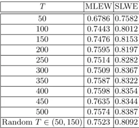
The classification procedure explained above was performed on multinomial data streams generated from two different classes where the probability of the distributions of each class switched four times. For the results which we report, each element of the data stream could take any of the four different values, namely 1, 2, 3 or 4. The specific values of Si1 and Si2, were changed and set to random values four times at random time instances, which were assumed to be unknown to the classifiers. The results are shown in Table 1, and again, the uniform superiority of the SLWE over the MLEW is noticeable. For example, when T=100, the MLEW-based classifier yielded an accuracy of only 0.7443, but the corresponding accuracy of the SLWE-based classifier was 0.8012. We also notice that the results of the classification in periodic environments with a varyingT chosen randomly from [50,150] were also similar to the fixedT = 100 case, as the classifier achieved the accuracy of 0.8092 and 0.8012 in the first and second environments, respectively. The results also show that the SLWE-based algorithm handles the concept drift and provides satisfactory performance.

T MLEW SLWE 50 0.6786 0.7582 100 0.7443 0.8012 150 0.7476 0.8153 200 0.7595 0.8197 250 0.7514 0.8282 300 0.7509 0.8367 350 0.7587 0.8322 400 0.7598 0.8354 450 0.7635 0.8344 500 0.7574 0.8387 RandomT ∈(50,150) 0.7523 0.8092

Table 1.The ensemble results for 100 simulations obtained from testing multinomial classifiers which used the SLWE (with λ = 0.9) and the MLEW for classifying one-dimensional data streams generated by two non-stationary different sources.

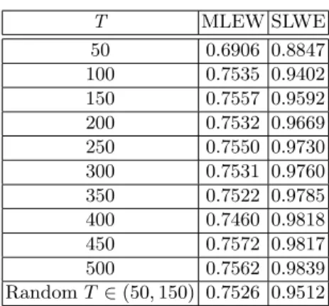
The experiment explained above was repeated on different 2-class multino-mial datasets with different dimensionalities. These sets were generated ran-domly based on random vectors with different random distribution probabilities involving 2, 3 and 4 dimensions and each element could take on four different values. The results obtained are shown in Tables 3-2, from which we see that classification using the SLWE was uniformly superior to classification using the MLEW. For example, for the 2-dimensional data, whenT= 250, the MLE-based classifier resulted in the accuracy of 0.7544 and the SLWE achieved significantly better results with the accuracy of 0.9706. Here the accuracy of the classifier,

(11)

Table 2.The ensemble results for 100 simulations obtained from testing multinomial classifiers which used the SLWE (with λ = 0.9) and the MLEW for classifying 4-dimensional data streams generated by two non-stationary different sources.

increased with the dimensionality of the datasets as the classifiers could process the data more efficiently. For example, in the case ofT = 150 the SLWE-based

online classifier resulted in the average accuracy of 0.9181 over several different two-dimensional datasets, while with more useful information in 4-dimensional datasets, it yielded better results with the accuracy of 0.9569.

Table 3.The ensemble results for 100 simulations obtained from testing multinomial classifiers which used the SLWE (with λ = 0.9) and the MLEW for classifying 2-dimensional data streams generated by two non-stationary different sources.

(12)

5 Conclusion

In this paper we have considered the problem of classification when these phases of training and testing are not so clearly well-defined, i.e., where the testing patterns can subsequently be considered as training patterns. This paradigm of classification is further complicated because we have assumed that the class-conditional distributions of the classes are time-varying or non-stationary. Here, we consider the scenario when the patterns arrive sequentially in the form of a data stream with potentially time-varying probabilities that change over time for each class. The proposedonlineclassification algorithm was used to perform the training and the testing simultaneously in three phases. In the first phase, the algorithm received a new unlabeled instance. After this, the scheme assigned a label to it based on the distributions’ estimated probabilities using the SLWE. Finally, after a few time instances, the algorithm received the actual class of the instance and used it to update the training model by invoking the SLWE updating algorithm. In this way the training and testing phases are almost in-tertwined. Thereafter, the classification model was adjusted to the new available instances in anonline manner.

References

1. A. Bifet. Adaptive Learning and Mining for Data Streams and Frequent Patterns. PhD thesis, Departament de Llenguatges i Sistemes Informatics, Universitat Politc-nica de Catalunya, Barcelona Area, Spain, 2009.

2. A. Bifet and R. Gavalda. Kalman Filters and Adaptive Windows for Learning in Data Streams. In L. Todorovski and N. Lavrac, editors, Proceedings of the 9th Discovery Science, volume 4265, pages 29–40, 2006.

3. A. Bifet and R. Gavalda. Learning From Time-changing Data With Adaptive Win-dowing. InProceedings SIAM International Conference on Data Mining, volume 8, pages 443–448, 2007.

4. J. Gama, P. Medas, G. Castillo, and P. Rodrigues. Learning with Drift Detection. In A. Bazzan and S. Labidi, editors,Advances in Artificial Intelligence SBIA 2004, volume 3171 ofLecture Notes in Computer Science, pages 286–295. Springer Berlin Heidelberg, 2004.

5. B. J. Oommen and L. Rueda. Stochastic Learning-based Weak Estimation of Multi-nomial Random Variables and Its Applications to Pattern Recognition in Non-stationary Environments. Pattern Recognition, 39(3):328–341, 2006.

6. G. Widmer and M. Kubat. Learning in the Presence of Concept Drift and Hidden Contexts. InMachine Learning, volume 23, pages 69–101, 1996.