University of Nebraska - Lincoln
DigitalCommons@University of Nebraska - Lincoln
Nebraska Department of Transportation ResearchReports Nebraska LTAP
12-2004
Safety Evaluation of Left Turn Lane Line Width at
Intersections with Opposing Left Turn Lanes
Aemal Khattak
University of Nebraska-Lincoln, [email protected]
Bhaven Naik
University of Nebraska-Lincoln, [email protected]
Vijay Kannan
Mid-America Transportation Center
Follow this and additional works at:https://digitalcommons.unl.edu/ndor
Part of theTransportation Engineering Commons
This Article is brought to you for free and open access by the Nebraska LTAP at DigitalCommons@University of Nebraska - Lincoln. It has been accepted for inclusion in Nebraska Department of Transportation Research Reports by an authorized administrator of DigitalCommons@University of Nebraska - Lincoln.
Khattak, Aemal; Naik, Bhaven; and Kannan, Vijay, "Safety Evaluation of Left Turn Lane Line Width at Intersections with Opposing Left Turn Lanes" (2004).Nebraska Department of Transportation Research Reports. 11.
NDOR Research Project Number SPR-P1(03) P554
Transportation Research Studies
F
I
N
A
L
R
E
P
O
R
T
SAFETY EVALUATION OF LEFT-TURN LANE
LINE WIDTH AT INTERSECTIONS WITH
OPPOSING LEFT TURN LANES
Prepared for
Nebraska Department of Roads
1500 Nebraska Highway 2
Lincoln, NE 68509-4759
By
Aemal J. Khattak, Bhaven Naik and Vijay Kannan
Mid-America Transportation Center
University of Nebraska-Lincoln
W333.2 Nebraska Hall
Lincoln, Nebraska 68588-0530
Telephone: (402) 472-1974
Fax: (402) 472-0859
Website: http://www.matc.unl.edu
December 2004
DISCLAIMER
The contents of this report reflect the views of the authors and do not necessarily reflect the official views or policies of the Nebraska Department of Roads, the Federal Highway Administration, or the University of Nebraska-Lincoln. This report does not constitute a standard, specification, or regulation. Trade or manufacturers’ names that appear in this report are cited only because they were essential to the objectives of this research. The appearances of trade or manufacturers’ names do not constitute endorsements.
EXECUTIVE SUMMARY
The objective of this research project was to evaluate the effectiveness of offset opposing left-turn lanes at signalized intersections in reducing the frequency and severity of left-turn related accidents. The Cities of Lincoln and Omaha offset opposing turns by widening left-turn lane lines in June 1999 at six intersections. The research team investigated traffic accident patterns between January 1994 and December 2002 at those six intersections by making
comparisons with two control intersections (i.e. intersections at which left-turns were not offset by lane line widening) using a four-step research methodology. First, existing literature was reviewed to determine the extent and availability of materials relevant to this project. Second, accident data were collected for the six study and two control intersections. The third step
involved the analysis of the collected data. Four analysis techniques were employed to assess the effectiveness of off-setting opposing left- turn lanes by using wider left-turn lanes lines.
Results from the trend analysis of accident frequencies and accident rates presented a mixed picture of the ‘before’ (pre-June 1999) and ‘after’ (post-June 1999) data. In the absence of a clear-cut increasing or decreasing trend in the accident frequencies and rates, the research team conducted an in-depth analysis of the collected data. Accident/crash rates were analyzed by using linear regression while accident frequencies were re-analyzed by the Before-After (B-A) analysis and by using Poisson regression modeling. Crash rate modeling showed mixed results since rates were increasing and decreasing at various intersections with time and either increased or
decreased in the ‘after’ time period. Only the 72nd and Cass intersection in Omaha appeared to
have experienced statistically significant crash rate reduction.
The B-A analysis of accident frequency was conducted using the simple and the
comparison group (C-G) methods. Overall, the simple method indicated that accident frequency decreased in the ‘after’ period. However, in the simple B-A analysis, the change in safety reflects upon all sundry factors such as traffic, weather, driver behavior etc. that might have changed between the ‘before’ and ‘after’ periods. The C-G method indicated that there was a decrease in the frequency of accidents in the ‘after’ period that can be attributed to offsetting opposing left-turns. The Poisson regression modeling of accident frequency took into consideration the effects of traffic at the intersections and indicated a limited reduction in the accident frequency in the ‘after’ period. The last part of the analysis was focused on injury severity – Ordered logit models
were estimated in this case. The models indicated that maximum injury severity decreased in the ‘after’ period after taking into account the traffic effects in the ‘before’ and ‘after’ periods.
The fourth step consisted of developing conclusions and recommendations for future research based on the results of this study. The research team concludes and recommends the following:
• Offsetting of opposing left-turn lanes by widening left-turn lane lines is effective in reducing accidents,
• The reduction in the expected accident frequency was about 0.285% however, the
reduction appears to be city-specific,
• Offsetting of opposing left-turn lanes by widening left-turn lane lines reduces accident injury severity.
The research team recommends continuation of the practice of off-setting opposing left-turn lanes, where feasible. For future research, the team recommends that additional factors (e.g., number of days with adverse weather in the ‘before’ and ‘after’ periods, construction activities at or near study locations, etc.) besides traffic must also be accounted for in the analysis.
TABLE OF CONTENTS
Page DISCLAIMER... i EXECUTIVE SUMMARY ... ii TABLE OF CONTENTS ... iv LIST OF FIGURES ... ivLIST OF TABLES... ivi
CHAPTER 1 - INTRODUCTION... 1
1.1. Background... 1
1.2. Objective... 1
1.3. Research Methodology ... 2
1.4. Report Organization... 2
CHAPTER 2 - LITERATURE REVIEW... 4
2.1. Information from Reviewed Literature... 4
2.2. Literature Summary ... 7
CHAPTER 3 – DATA COLLECTION AND ANALYSIS... 8
3.1. Treated Sites... 8
3.2. Control Sites... 8
3.3. Lane Offset Implementation ... 10
3.4. Data Collection ... 17
3.4.1. Accident Data... 17
3.4.2. Traffic Data... 19
3.5. Data Analysis... 21
3.5.1. Time Trend Analysis... 21
3.5.2. Accident/Crash Rate Analysis ... 29
3.5.3. Accident Frequency Analysis ... 31
3.5.3.1. Before-After Analysis... 31
3.5.3.2. Poisson Regression Modeling... 36
3.5.4. Injury Severity Analysis ... 39
CHAPTER 4 – CONCLUSIONS AND RECOMMENDATIONS ... 43
4.1. Research Summary ... 43
4.2. Conclusions and Recommendations ... 44
ACKNOWLDGMENTS... 46
LIST OF FIGURES
Page
1.1. Research methodology...3
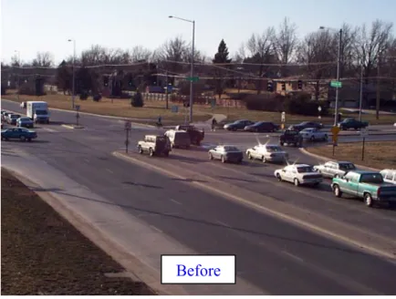
3.1. Before and after left-turn lane lines at 27th and Highway 2...11
3.2. Before and after left-turn lane lines at 70th and Van Dorn St. ...12
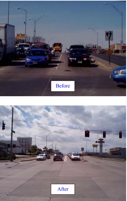
3.3. Before and after left-turn lane lines at 48th and ‘O’ St...13
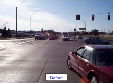
3.4. Before and after left-turn lane lines at 70th and ‘O’ St...14
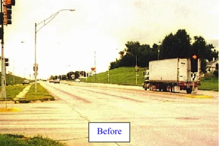
3.5. Before and after left-turn lane lines at 60th and ‘L’ St. ...15
3.6. Before and after left-turn lane lines at 72nd and Cass St. ...16
3.7. a. Accident frequency trends for individual intersections ...22
b. Accident frequency trends for individual intersections ...23
3.8. Accident frequency trends for Lincoln, Omaha, and Control Intersections ...24
3.9. Accident frequency trends for Treated and Control Intersections ...24
3.10. a. Crash rate trends for individual intersections...26
b. Crash rate trends for individual intersections ...27
3.11. Crash rate trends for Lincoln, Omaha and Control Intersections ...28
LIST OF TABLES
Page
2.1. Minimum and desirable left-turn offsets...5
3.1. Characteristics of the Treated intersections ...9
3.2. Characteristics of the Control intersections ...9
3.3. Left-turn lane-line widths effected at Treated intersections ...10
3.4. Accident frequency by severity ...18
3.5. Yearly availability of ADT data ...20
3.6. Fitted models used to estimate yearly ADT...20
3.7. Estimated yearly ADT ...21
3.8. Statistical Data for Comparison of Mean accident frequencies...25
3.9. Accident rate regression models for individual intersections ...30
3.10. Pooled Lincoln and Omaha accident rate models...30
3.11. Pooled Treated and Control accident rate models ...30
3.12. Formulae for Simple Before-After analysis...32
3.13. Citywide results of Simple Before-After analysis ...32
3.14. Control results of Simple Before-After analysis ...33
3.15. Combined Treated results of Simple Before-After analysis ...33
3.16. Formulae for C-G Before-After analysis ...34
3.17. Citywide results of C-G Before-After analysis ...35
3.18. Combined results of C-G Before-After analysis ...35
3.19. Poisson accident frequency models for Lincoln, Omaha, & combined data ...38
Chapter 1 INTRODUCTION
1.1. Background
Vehicles in opposing left-turn lanes obstruct each other’s view of the oncoming traffic streams through which they must turn i.e. restrict each other’s sight distance. Previous research conducted by McCoy et al., (1992) for the Nebraska Department of Roads (NDOR) developed guidelines for offsetting opposing left-turn lanes to provide adequate sight distances. However, any implementation of these guidelines at existing intersections typically meant reconstruction of the left-turn lanes. Subsequent research by McCoy et al., (1999) found that widening the lane lines between the left-turn lanes and the adjacent through lanes could also improve the sight distance and this strategy was more economical than the reconstruction of existing intersections. Utilizing the relationship found between lane line width and available sight distance, guidelines for designing the width of left-turn lane lines to provide the required sight distance for opposing left-turn vehicles without reconstruction were developed.
In June 1999, the Cities of Lincoln and Omaha in cooperation with NDOR widened the left-turn lane lines at several intersections on arterial streets and urban sections of the State highway system. Although increasing the available sight distance for left-turn vehicles would intuitively seem to reduce left-turn related accidents, the safety effects of wider left-turn lane lines have not been documented. Without this knowledge of the effects of wider left-turn lane lines on the frequency and severity of left-turn related accidents, it is not possible to assess the safety benefits and cost effectiveness of widening these lane lines. If they have no effect on safety, then their additional cost is not justified.
1.2. Research Objective
The objective of the research described in this report was to evaluate the safety
effectiveness of widening left-turn lane lines in reducing the frequency and severity of left-turn related accidents at signalized intersections with opposing left-turn lanes. The research emphases were based on an analysis in which control intersections (i.e. where left-turn lane lines were not widened) are used to evaluate the effects of widening left-turn lane lines.
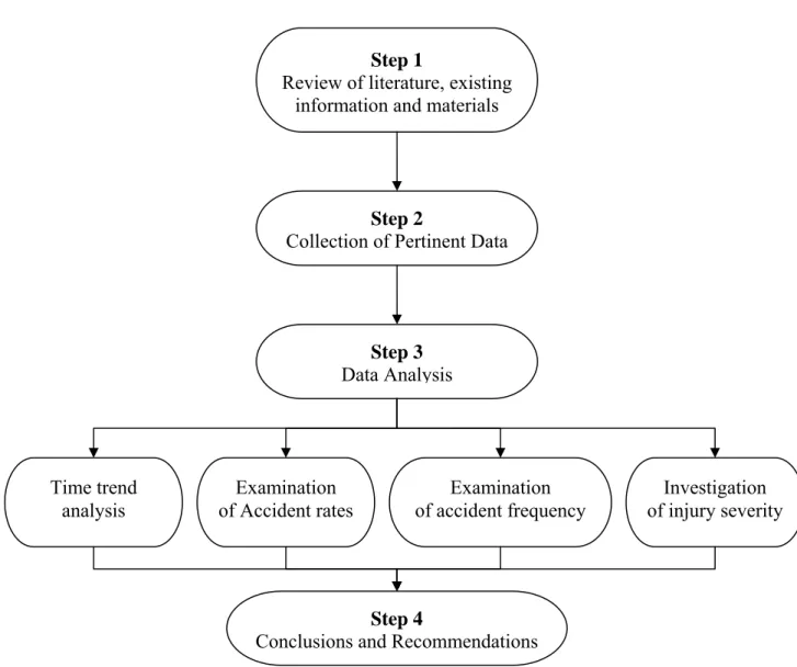
1.3. Research Methodology
The research methodology consisted of four steps as illustrated in Figure 1.1. Step 1 involved a review of existing literature to determine the extent and the availability of materials relevant to this project. This review was focused on literature related to offset left-turn lanes, sight distance, safety benefits due to offsetting left-turn lanes, and B-A road safety studies. Step 2 involved the collection of nine years (1994 - 2002) of accident data. The data collected were for six study intersections (four in Lincoln and two in Omaha) at which the left-turn lane line was widened. Additional accident data were also collected for two control intersections at which the left-turn lane line was not widened. The collected data were analyzed in the third step by using four different analysis techniques. These include the time trend analysis, examination of accident rates, examination of accident frequency, and investigation of injury severity. Conclusions on the research and recommendations for future research were made in the final step.
1.4. Report Organization
This report consists of a total of four chapters. This introductory chapter is followed by a chapter that provides details of the literature review and the information exposed on the subject matter. Chapter Three presents details of the collected data and its analysis. Chapter Four presents the research conclusions and recommendations for future research.
Step 1
Review of literature, existing information and materials
Step 2
Collection of Pertinent Data
Step 3 Data Analysis
Figure 1.1. Research Methodology Time trend analysis Examination of Accident rates Examination of accident frequency Investigation of injury severity Step 4
Chapter 2
LITERATURE REVIEW
As part of the literature review, several documents were examined to identify pertinent information on the safety effects of left-turn offsets at intersections with opposing left turn lanes as well as information on conducting B-A studies. This information is presented next while a summary of the literature review is provided at the end of the chapter.
2.1. Information from Reviewed Literature
Mitchell (1972) conducted a one-year B-A study (i.e., a B-A study with one year duration at both ends) of intersections where a variety of improvements were implemented. The results showed a 67 percent reduction (from 39 to 13) in accidents where obstructions that inhibited sight distance were removed; this was the most effective of the implemented improvements.
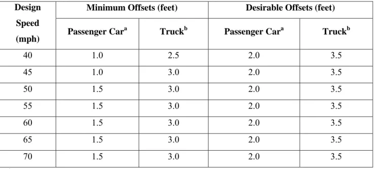
McCoy et al., (1992) developed guidelines for offsetting opposing left-turn lanes to provide adequate sight distance for permitted left-turn movements from opposing left-turn lanes. These guidelines focused on the minimum offsets needed to provide adequate sight distances to left-turning vehicles positioned at the stop line and opposed by left-turn vehicles positioned within the intersection. All offsets specified in the guidelines were positive indicating that the negative offsets that typically exist between opposing left-turn lanes at these locations do not provide adequate sight distances for opposing left-turn vehicles. For 90-degree intersections on level, tangent sections of four-lane divided roadways with 12-ft left-turn lanes in 16-ft medians with 4-ft median separators, the following conclusions were stated by McCoy et al.,: (1) a 2-ft positive offset provides unrestricted sight distance when the opposite left-turn vehicle is a passenger car, and (2) a 3.5-ft positive offset provides unrestricted sight distance when the opposite left-turn vehicle is a truck, for design speeds up to 70 mph. The minimum offsets needed between opposite left-turn lanes to provide adequate sight distance were determined by equating the available sight distance equations to the required sight distance equation and solving for the offset. Table 2.1 shows the minimum and desirable offsets determined by McCoy et al. (1992).
Table 2.1. Minimum and Desirable Left-Turn Offsets
Minimum Offsets (feet) Desirable Offsets (feet)
Design Speed
(mph) Passenger Car
a
Truckb Passenger Cara Truckb
40 1.0 2.5 2.0 3.5 45 1.0 3.0 2.0 3.5 50 1.5 3.0 2.0 3.5 55 1.5 3.0 2.0 3.5 60 1.5 3.0 2.0 3.5 65 1.5 3.0 2.0 3.5 70 1.5 3.0 2.0 3.5
a Opposing left-turn vehicle is a passenger car Source:(McCoy et al., 1992)
b Opposing left-turn vehicle is a truck
The offset can be achieved by simply widening the left-turn lane line as indicated from research conducted by McCoy et al., (1999) on the effectiveness of wider left-turn lane lines in improving sight distance from opposing turn lanes. The research showed that vehicles in opposing left-turn lanes positioned themselves significantly closer to the median when the wider lane lines were in place and as such had adequate sight distances. In addition, guidelines to calculate minimum left-turn lane line widening were developed.
Joshua and Saka (1992) reported that sight distance problems at intersections which result from queued vehicles in opposite left-turn lanes pose safety and capacity deficiencies, particularly for unprotected (permitted) left-turn movements. These researchers found a strong correlation between the offset for opposite turn lanes and the available sight distance for left-turning traffic. However, the authors did not perform any accident investigation to show the effectiveness. A study conducted by Bonneson et al., (1993) reported that although about one-third of the state highway departments have successfully used the offset design at selected locations, there is no substantial research conducted on quantifying the safety benefits.
Harwood et al., (1995) stated that wider medians generally have positive effects on traffic operations and safety; however, wider medians can result in sight restrictions for left-turning
vehicles resulting from the presence of opposite left-turn vehicles. The most common solution suggested by the author was to offset the left-turn lanes, using either parallel offset or tapered offset left-turn lanes. The authors found no major traffic operational or safety problems at three signalized intersections with offset left-turn lanes.
Staplin, et al., (1996) performed a laboratory study, field study, and sight distance analysis to measure driver age differences in performance under varying traffic and operating conditions, as a function of varying degrees of offset of opposite left-turn lanes at suburban arterial intersections. In the field study, where left-turn vehicles needed to cross the paths of two or three lanes of conflicting traffic (excluding parking lanes) at 90-degree, 4-legged intersections, four levels of offset of opposite left-turn lane geometry were examined as follows: (a) 6-ft "partial positive" offset, (b) aligned (no offset) left-turn lanes, (c) 3-ft "partial negative" offset, and (d) 14-ft "full negative" offset. All intersections were located within a growing urban area where the posted speed limit was 35 mph. Additionally, all intersections were controlled by traffic-responsive semi-actuated signals, and all left-turn maneuvers were completed during the permissive left-turn phase at all study sites. In the analysis of the field study lateral positioning data, it was found that the partial positive offset and aligned locations had the same effect on the lateral positioning behavior of drivers. At the same time, drivers moved approximately 5 ft to the left when there was a large negative offset (-14 ft), clearly indicating that sight distance was limited. There was also significant difference between the partial negative offset geometry (-3 ft) versus the partial positive offset and aligned geometries, suggesting a need for longer sight distance when opposite left-turn lanes are even partially negatively offset. The fact that older drivers (and females) were less likely to position themselves (i.e., pull into the intersection) in the field studies highlighted the importance of providing adequate sight distance for unpositioned drivers.
Further studies by Tarawneh and McCoy (1996, 1997) developed guidelines for other vehicle types and positioning scenarios. But implementation of these guidelines at existing intersections typically involved reconstruction of the left-turn lanes. The relatively high cost of such reconstruction often prohibits, or at least delays, the elimination of sight distance problems at existing intersections.
A review of the AASHTO’s “A Policy on Geometric Design of Highways and Streets” (commonly known as the “Green Book”, 2001) indicated that the provision of adequate sight distance at opposing left-turn lanes is desirable and suggests the use of parallel or tapered offsets as a means of improving sight distance. However, it does not specify the amount of offset required.
2.2. Literature Summary
In summary, the literature review indicated that offsetting opposing left-turn lanes increased sight distance for permitted left-turn movements from opposing left-turn lanes. Implementation of this strategy at an existing intersection by widening the lane line between left turning lane and the adjacent through lane is more economical than reconstruction. Most of the research in this area has been focused on the development of guidelines for offsetting opposing left-turn lanes for different scenarios. Even though about one-third of the state highway departments have successfully used the offset design at selected locations, the safety benefits of offsetting the left turn lane have not yet been quantified.
Chapter 3
DATA COLLECTION AND ANALYSIS
Evaluation of the safety effectiveness of projects implemented at treatment sites requires a method for estimating the changes in safety that would have occurred at the treatment sites had the improvements not been made. This is normally accomplished with data from sites that are not treated during the study period. For this purpose the evaluation intersections were classified into two groups as follows;
• Treated or Improved – which were intersections at which the left-turn lanes were offset.
• Control or Comparison – which were intersections with similar characteristics as the
treated intersections but, were not treated.
This chapter provides information on the characteristics of the eight evaluation intersections i.e. six treated intersections and two control intersections and the nine-year accident and traffic data collected for these intersections. Analysis of the collected data is also a part of this chapter. 3.1. Treated Sites
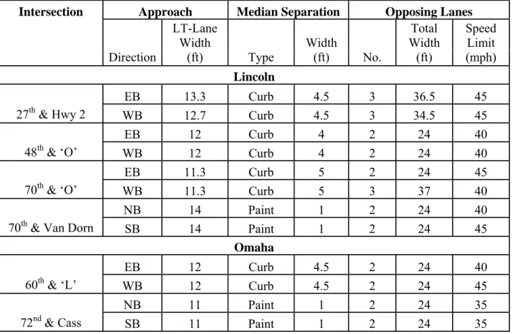
The six treated sites were intersections with left-turn lanes on opposing approaches on arterial streets in the Cities of Lincoln and Omaha, Nebraska. Four of the intersections were located in Lincoln and two were located in Omaha. All the six intersections selected were right-angled, signalized intersections with protected/permitted left-turn phases. However, they varied with respect to lane widths, median type, median width, and left-turn lane offset. The characteristics of these treated intersections are summarized in Table 3.1.
3.2. Control Sites
These were selected by the technical advisory committee on the basis of similarities in characteristics with the four study intersections in Lincoln. The two control intersections with left-turn lanes on opposing approaches on arterial streets were located in Lincoln. The
Table 3.1. Characteristics of the Treated Intersections
Intersection Approach Median Separation Opposing Lanes
Direction LT-Lane Width (ft) Type Width (ft) No. Total Width (ft) Speed Limit (mph) Lincoln EB 13.3 Curb 4.5 3 36.5 45
27th & Hwy 2 WB 12.7 Curb 4.5 3 34.5 45
EB 12 Curb 4 2 24 40
48th & ‘O’ WB 12 Curb 4 2 24 40
EB 11.3 Curb 5 2 24 45
70th & ‘O’ WB 11.3 Curb 5 3 37 40
NB 14 Paint 1 2 24 40
70th & Van Dorn SB 14 Paint 1 2 24 45
Omaha
EB 12 Curb 4.5 2 24 40
60th & ‘L’ WB 12 Curb 4.5 2 24 45
NB 11 Paint 1 2 24 35
72nd & Cass SB 11 Paint 1 2 24 35
intersections were right-angled, signalized with protected/permitted left-turn phases but without offset left-turns. The characteristics of these control intersections are summarized in Table 3.2.
Table 3.2. Characteristics of the Control Intersections
Intersection Approach Median Separation Opposing Lanes
Direction
LT-Lane Width
(ft) Type Width (ft) No.
Total Width (ft) Speed Limit (mph) NB 12 Curb 4 2 24 40
27th and ‘O’ SB 12 Curb 4 2 24 40
NB 12 Curb 4 2 24 40
3.3. Lane Offset Implementation
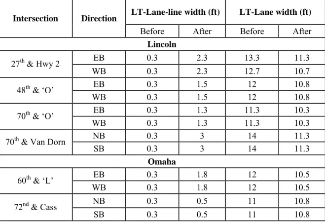
The left-turn lane line widths shown in Table 3.3 were implemented at the six treated intersections by painting pavement markings over the existing 4-inch left-turn lane lines. The particular pavement marking pattern used depended on the width of the new lane lines. At the intersections of 27th and Highway 2 and 70th and Van Dorn, the new left-turn lane line widths were sufficient to enable tapered channelization islands to be painted over the existing lane lines as shown in Figures 3.1 and 3.2. For the narrower left-turn lane-line widths at the other study sites, one of two patterns was used. In Lincoln, the increase in lane-line width was achieved by using double solid lines in place of the existing lines. This was implemented at the intersections of 48th and ‘O’ Street and 70th and ‘O’ Street as shown in Figures 3.3 and 3.4. In Omaha, a single solid line was used to increase the lane line widths at 60th and ‘L’ Street and 72nd and Cass Street. These single solid lines are shown in Figures 3.5 and 3.6.
Table 3.3. Left-Turn Lane-Line Widths Effected at Treated Intersections
LT-Lane-line width (ft) LT-Lane width (ft)
Intersection Direction
Before After Before After Lincoln EB 0.3 2.3 13.3 11.3 27th & Hwy 2 WB 0.3 2.3 12.7 10.7 EB 0.3 1.5 12 10.8 48th & ‘O’ WB 0.3 1.5 12 10.8 EB 0.3 1.3 11.3 10.3 70th & ‘O’ WB 0.3 1.3 11.3 10.3 NB 0.3 3 14 11.3 70th & Van Dorn
SB 0.3 3 14 11.3 Omaha EB 0.3 1.8 12 10.5 60th & ‘L’ WB 0.3 1.8 12 10.5 NB 0.3 0.5 11 10.8 72nd & Cass SB 0.3 0.5 11 10.8
Before
After
Before
After
Before
After
Before
After
Before
After
Before
After
3.4. Data Collection
The treated sites consisted of six intersections – four in Lincoln and two in Omaha. The four intersections in Lincoln were 27th and Highway 2, 48th and ‘O’, 70th and ‘O’, and 70th and Van Dorn. The two intersections in Omaha were at 60th and ‘L’, and 72nd and Cass. The two control intersections were based in Lincoln at 27th and ‘O’ and 70th and South St.
The study period was from January 1994 to December 2002. The ‘before’ study period was from January 1994 to June 1999 and the ‘after’ study period was from July 1999 to December 2002, because changes were made to the intersections around June 1999.
3.4.1. Accident Data
Police crash reports were obtained from the Cities of Lincoln and Omaha for the 9-year study period (1994 – 2002). Data obtained from the City of Omaha included accident reports related to left-turn accidents at the two study intersections while data obtained from the City of Lincoln included all accidents reported at the four treated and two control intersections in Lincoln.
To reduce the Lincoln data to only left-turn related accidents, the code containing information on whether the accident was left-turn related was used. To reduce the possibility of missing any left-turn related accidents by relying on the left-turn code, the research team checked a sample of 50 accidents reported in through lanes to evaluate if any of those were related to left- turns in any way. The research team did not find evidence that any of the inspected accidents were related to left-turns. Therefore, it was assumed that none of the 6,000 accidents reported in the through lanes were related to the left-turn and all accidents reported in through lanes in Lincoln were excluded from the analysis. The number, fifty, was selected based on considerations of convenience and availability of resources rather than any sample size calculations. Sample size calculations were not possible because the formula required knowledge of sample standard deviation, which was unknown. Also, accidents reported on the minor approaches of the study intersections were excluded from the analysis since the left-turns were not offset on these approaches. Overall there were 298 accidents that qualified for data analysis. Attributes obtained from the accident reports included fields such as date of accident, case ID, location, weekday, time of accident and injury severity.
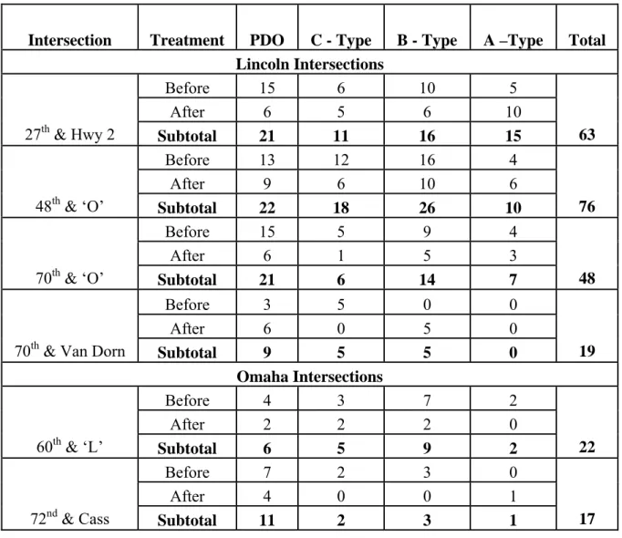
The 298 accidents were pooled into 3-month, 6-month and 1-year time periods for each intersection. Since there were no significant differences in the patterns over these three time periods, the 6-month time period was considered for further analysis. Table 3.4 shows the total number of accidents by maximum injury severity (injury measured on the KABCO scale – Killed, A-type injury, B-type injury, C-Type injury, and Property-Damage-Only) for each intersection. Fatalities were not recorded at any of the intersections during the study period.
Table 3.4. Accident Frequency by Severity
Intersection Treatment PDO C - Type B - Type A –Type Total
Lincoln Intersections
Before 15 6 10 5
After 6 5 6 10
27th & Hwy 2 Subtotal 21 11 16 15 63
Before 13 12 16 4
After 9 6 10 6
48th & ‘O’ Subtotal 22 18 26 10 76
Before 15 5 9 4
After 6 1 5 3
70th & ‘O’ Subtotal 21 6 14 7 48
Before 3 5 0 0
After 6 0 5 0
70th & Van Dorn Subtotal 9 5 5 0 19
Omaha Intersections Before 4 3 7 2 After 2 2 2 0 60th & ‘L’ Subtotal 6 5 9 2 22 Before 7 2 3 0 After 4 0 0 1
Table 3.4. (continued) Accident Frequency by Severity
Intersection Treatment PDO C - Type B - Type A –Type Total
Control Intersections Before 14 5 0 0 After 17 0 0 1 27th &'O' Subtotal 31 5 0 1 37 Before 5 4 0 0 After 2 2 3 0
70th & South Subtotal 7 6 3 0 16
Overall Total 128 58 76 36 298
3.4.2. Traffic Data
The actual measured average daily traffic (ADT) information for the intersections in the two Cities was only available for the years shown in Table 3.5. Traffic on the minor approaches (where the left lane was not offset) was excluded from traffic counts at all eight intersections. The right turning traffic volume on the North and South bound approaches at the 72nd and Cass intersection and the right turning traffic on the Southbound approach at the 27th and Hwy 2 intersection were excluded as these approaches have ramp-like right turning lanes. The adjusted traffic data were used to interpolate the yearly ADT on the major approaches for each year of the 9-year study period. Table 3.6 presents the regression models used to interpolate the ADT. All the intersections except 48th and ‘O’ and the control at 70th and South St. had linear models with
reasonable R2 (the coefficient of determination in linear regression) values. Due to the
availability of three years of ADT data for the intersections at 48th and ‘O’ and 70th and South St., the researchers opted to estimating quadratic regression models. Therefore quadratic regression models were estimated to predict the ADT for these two intersections. Table 3.7 shows the estimated yearly ADT data during the study period.
Table 3.5. Yearly Availability of ADT Data
Lincoln Omaha Control
27th & Hwy 2 48th & ‘O’ 70th & ‘O’ 70th & Van Dorn 60th & ‘L’ 72nd & Cass 27th & ‘O’ 70th & South 1991 1991 1991 1991 1990 1988 1998 1993 1992 1995 1992 1992 2001 1991 2001 2000 1993 1997 1993 1994 1996 2002 1994 1994 1995 1998 1996 1995 1996 1997 1997 1997 1998 2000
Table 3.6. Fitted Models used to Estimate Yearly ADT
Intersection Estimated ADT Model R2
Lincoln
27th and Hwy2 y = 787.56x + 27596 0.62
48th and 'O' y = 170.83x2 - 1525x + 41354 1.00
70th and 'O' y = 405.71x + 25196 0.92
70th and Van Dorn y = 145.99x + 6290.3 0.94
Omaha 60th and 'L' y = 276.73x + 26952 1.00 72nd and Cass y= 223.46x + 28292 0.60 Controls 27th and 'O' y = 2.1679x + 4340.4 1.00 70th and South y = -10.56x2 + 336.64x + 7454.9 1.00
Note: i. x represents the period (i.e., 1994 = 1, 1995 = 2, ………, and 2002 = 9);
ii. R2 values of 1.00 are obtained because there are only three data points for intersections at 48th and ‘O’ and 70th and South and only two data points in the case of 60th and ‘L’.
Table 3.7. Estimated Yearly ADT Year 1994 1995 1996 1997 1998 1999 2000 2001 2002 Intersection Lincoln 27thand Hwy 2 30746 31534 32321 33109 33896 34684 35472 36259 37047 48th and 'O' 37987 38000 38354 39050 40087 41466 43187 45249 47654 70thand ‘O’ 26819 27225 27630 28036 28442 28847 29253 29659 30065
70thand Van Dorn 6874 7020 7166 7312 7458 7604 7750 7896 8042
Omaha 60thand ‘L’ 28336 28612 28889 29166 29443 29719 29996 30273 30549 72ndand Cass 29856 30080 30303 30527 30750 30974 31197 31420 31644 Controls 27thand ‘O’ 8663 8665 8668 8670 8672 8674 8676 8678 8681 70thand South 8086 8370 8632 8874 9094 9294 9472 9629 9765 3.5. Data Analysis
The safety benefits of left-turn offsets were evaluated by employing the following; i. B-A investigation of trends over time,
ii. Regression analysis of accident rates,
iii. Examination of accident frequency using B-A analysis and Poisson accident frequency modeling; and
iv. Ordered logit injury severity modeling.
Analysis by each of these four techniques is described next.
3.5.1. Time trend analysis
The accident frequency (accidents per 6-month period) and crash rates, for each intersection, were plotted against time to study their respective trends. Figure 3.7 (a and b) present the 6-month accident frequency trends at individual intersections. The x-axis represents time in 6-month intervals while the y-axis represents the frequency of accidents in a 6-month period. June 1999 represents the period in time when theintersections were treated (i.e. left-turns were offset). No distinct trends were visible for either treated or control intersections in the ‘before’ (i.e., pre June 1999) and ‘after’ (i.e., post June 1999) time periods except at the 60th and ‘L’ intersection, where there appears to be a decreasing trend in accident frequency over time.
27th St. and Hwy 2 0 1 2 3 4 5 6 7 8 9 199 4-1 199 4-2 199 5-1 199 5-2 199 6-1 199 6-2 199 7-1 199 7-2 199 8-1 199 8-2 199 9-1 199 9-2 200 0-1 200 0-2 200 1-1 200 1-2 200 2-1 200 2-2 Year 6 -m o nt h Ac c id e nt Fr e q 48th St. and 'O' St. 0 1 2 3 4 5 6 7 8 9 199 4-1 199 4-2 199 5-1 199 5-2 199 6-1 199 6-2 199 7-1 199 7-2 199 8-1 199 8-2 199 9-1 199 9-2 200 0-1 200 0-2 200 1-1 200 1-2 200 2-1 200 2-2 Year 6 -m o n th A c c ide nt Fr e q . 70th St. and 'O' St. 0 1 2 3 4 5 6 19 94 -1 19 94 -2 19 95 -1 19 95 -2 19 96 -1 19 96 -2 19 97 -1 19 97 -2 19 98 -1 19 98 -2 19 99 -1 19 99 -2 20 00 -1 20 00 -2 20 01 -1 20 01 -2 20 02 -1 20 02 -2 Year 6 -m o n th A c c ide nt F re q .
70th St. and Van Dorn
0 0.5 1 1.5 2 2.5 3 3.5 19 94-1 19 95-1 19 96-1 19 97-1 19 98-1 19 99-1 20 00-1 20 01-1 20 02-1 Year 6 -m o n th Ac c ide nt F re q . 60th St. and 'L' St. 0 0.5 1 1.5 2 2.5 1994-1 1995-1 1996-1 1997-1 1998-1 1999-1 2000-1 2001-1 2002-1 Year 6 -m ont h A c c id e n t Fr e q . 72nd St. and Cass 0 0.5 1 1.5 2 2.5 3 3.5 199 4-1 199 5-1 199 6-1 199 7-1 199 8-1 199 9-1 200 0-1 200 1-1 200 2-1 Year 6 -m ont h Ac c ide nt Fr e q .
70th St. and South - Control 0 0.5 1 1.5 2 2.5 1994-1 1995-1 1996-1 1997-1 1998-1 1999-1 2000-1 2001-1 2002-1 Year 6 -m o n th A c c ide nt Fr e q .
27th St. and 'O' St. - Control
0 1 2 3 4 5 6 1994-1 1994-2 1995-1 1995-2 1996-1 1996-2 1997-1 1997-2 1998-1 1998-2 1999-1 1999-2 2000-1 2000-2 2001-1 2001-2 2002-1 2002-2 Year 6 -m o n th Ac c ide n t Fr e q .
Figure 3.7.b. Accident Frequency Trends for Individual Intersections
Pooled data for the control intersections and treated intersections in each city (i.e., separate for Lincoln and Omaha) were plotted to study Citywide trends in relation to controls. Combined city and control intersection data were also plotted. Figures 3.8 and 3.9 present Citywide trends as well as trends for the combined and control data respectively. Although the trends are mixed, there appears to be a slight increasing trend in Lincoln in the ‘after’ period whereas there is an evident decrease in the Omaha trend. From Figure 3.9, it can be seen that there is a slight decreasing trend in the treated intersections in comparison to the control intersection trend. Note however, that these trends do not take into account other factors (e.g., traffic) that might have changed during the ‘before’ and ‘after’ time periods.
Pooled Citywide Vs Control data
0 2 4 6 8 10 12 14 16 18 20 1994-1 1995-1 1996-1 1997-1 1998-1 1999-1 2000-1 2001-1 2002-1Year
6-m
o
nt
h A
cc
ide
nt
F
re
q
Lincoln Omaha ControlsFigure 3.8. Accident Frequency Trends for Lincoln, Omaha and Control Intersections
Treated Vs Control data
0 2 4 6 8 10 12 14 16 18 20 1994-1 1995-1 1996-1 1997-1 1998-1 1999-1 2000-1 2001-1 2002-1
Year
6
-m
o
nt
h A
cc
ide
nt
F
re
q
Treated
Control
A statistical comparison of mean accident frequencies in the before-after period was also conducted and the results shown in Table 3.8. Although the results were not statistically significant at the 95% confidence level (i.e., p-value > 0.05), Table 3.8 shows that in respect to the individual intersections, there was an increase in the mean accident frequency in the ‘after’ period except at 70th and ‘O’, 60th and ‘L’ and, 72nd and Cass. The pooled data shows that there was a decrease in mean accident frequency at intersections in the City of Omaha. In relation to the combined treated and control intersection data, an increase in mean accident frequency can be noticed at the control as opposed to the treated intersections where there was no noticeable change in mean accident frequency.
Table 3.8. Statistical Data for Comparison between Means
Intersection Before After Mean Difference t-statistic p-value
Lincoln
27th and Hwy 2 3.27 3.86 -0.59 -0.62 0.54
48th and ‘O’ 4.09 4.43 -0.34 -0.38 0.71
70th and ‘O’ 3.00 2.14 0.86 1.14 0.27
70th and Van Dorn 0.73 1.57 -0.84 -1.65 0.12
Omaha 60th and ‘L’ 1.36 0.86 0.50 1.37 0.19 72nd and Cass 1.09 0.71 0.38 1.24 0.23 Controls 27th and ‘O’ 1.73 2.57 -0.84 -1.43 0.17 70th and South 0.82 1.00 -0.18 -0.44 0.66 Pooled Lincoln 11.09 12.00 -0.91 -0.55 0.59 Omaha 2.45 1.57 0.88 1.80 0.09 Controls 2.54 3.57 -1.03 -1.87 0.07 Treated 13.54 13.57 -0.03 -0.02 0.99
Note: i. the negative t-statistic indicates that there was an increase in the accidents in the ‘after’
period. This is similar to the negative sign for the mean difference.
ii. assumed there are unequal variances due to different sample sizes.
Similar investigative observations as for the accident frequency were conducted, but this time around the research team used Crash rate trends. The intersection crash rate for each 6-month period was calculated using:
106 ) ( × × =
∑
∑
A D T CR (3.1) Where:CR = crash rate (accidents per million entering vehicles), T = number of accidents in a 6-month period,
D = 180 days (average number of days in a 6-month period),
A = average daily traffic (vehicles per day) on the major approach where the left lane was offset minus right turning traffic on intersections with ramp-like right turn lane. Figures 3.10 (a and b), 3.11, and 3.12 present the crash rate trends for individual intersections, Citywide (Lincoln and Omaha), and combined treated and control intersections respectively. Individual intersections show significant variability in the trends and it is difficult to discern a clear trend in the accident rates except at the 60th and ‘L’ intersection, where the trend in crash rate appears to decrease with time. The citywide Lincoln and Omaha accident rates indicate that rates somewhat decreased in the ‘after’ period when compared to the controls. Figure 3.12 shows that there was a decrease in crash rates at the treated intersections in comparison with the control intersections. 27th St. and Hwy 2 0.00 0.20 0.40 0.60 0.80 1.00 1.20 1.40 1994-1 1994-2 1995-1 1995-2 1996-1 1996-2 1997-1 1997-2 1998-1 1998-2 1999-1 1999-2 2000-1 2000-2 2001-1 2001-2 2002-1 2002-2 Year 6 -m ont h C ra s h Ra te 48th St. and 'O' St. 0.00 0.20 0.40 0.60 0.80 1.00 1.20 1994-1 1994-2 1995-1 1995-2 1996-1 1996-2 1997-1 1997-2 1998-1 1998-2 1999-1 1999-2 2000-1 2000-2 2001-1 2001-2 2002-1 2002-2 Year 6 -m ont h Cr a s h Ra te
70th St. and 'O' St. 0.00 0.20 0.40 0.60 0.80 1.00 1.20 1994 -1 1994 -2 1995 -1 1995 -2 1996 -1 1996 -2 1997 -1 1997 -2 1998 -1 1998 -2 1999 -1 1999 -2 2000 -1 2000 -2 2001 -1 2001 -2 2002 -1 2002 -2 Year 6 -m ont h Cr a s h R a te
70th St. and Van Dorn
0.00 0.50 1.00 1.50 2.00 2.50 199 4-1 199 4-2 199 5-1 199 5-2 199 6-1 199 6-2 199 7-1 199 7-2 199 8-1 199 8-2 199 9-1 199 9-2 200 0-1 200 0-2 200 1-1 200 1-2 200 2-1 200 2-2 Year 6 -m ont h Cr a s h Ra te 60th St. and 'L' St. 0.00 0.10 0.20 0.30 0.40 0.50 19 94 -1 19 94 -2 19 95 -1 19 95 -2 19 96 -1 19 96 -2 19 97 -1 19 97 -2 19 98 -1 19 98 -2 19 99 -1 19 99 -2 20 00 -1 20 00 -2 20 01 -1 20 01 -2 20 02 -1 20 02 -2 Year 6-m o n th C ras h R a te 72nd St. and Cass 0.00 0.10 0.20 0.30 0.40 0.50 0.60 19 94 -1 19 94 -2 19 95 -1 19 95 -2 19 96 -1 19 96 -2 19 97 -1 19 97 -2 19 98 -1 19 98 -2 19 99 -1 19 99 -2 20 00 -1 20 00 -2 20 01 -1 20 01 -2 20 02 -1 20 02 -2 Year 6 -m o nt h Cr a s h Ra te
27th St. and 'O' St.- Control
0.00 0.50 1.00 1.50 2.00 2.50 3.00 3.50 19 94-1 19 94-2 19 95-1 19 95-2 19 96-1 19 96-2 19 97-1 19 97-2 19 98-1 19 98-2 19 99-1 19 99-2 20 00-1 20 00-2 20 01-1 20 01-2 20 02-1 20 02-2 Year 6-m o n th C rash R a te
70th St. and South St.- Control
0.00 0.20 0.40 0.60 0.80 1.00 1.20 1.40 19 94-1 19 94-2 19 95-1 19 95-2 19 96-1 19 96-2 19 97-1 19 97-2 19 98-1 19 98-2 19 99-1 19 99-2 20 00-1 20 00-2 20 01-1 20 01-2 20 02-1 20 02-2 Year 6 -m ont h Cr a s h Ra te
Pooled Citywide Vs Control Data
0.00 0.50 1.00 1.50 2.00 2.50 3.00 3.50 4.00 4.50 1994-1 1994-2 1995-1 1995-2 1996-1 1996-2 1997-1 1997-2 1998-1 1998-2 1999-1 1999-2 2000-1 2000-2 2001-1 2001-2 2002-1 2002-2 Year 6 -m o nt h C ra s h R a te Lincoln Omaha ControlsFigure 3.11. Crash Rate Trends for Lincoln, Omaha and Control Intersections
Treated Vs Control Data
0.00 0.50 1.00 1.50 2.00 2.50 3.00 3.50 4.00 4.50 5.00 19 94 -1 19 94 -2 19 95 -1 19 95 -2 19 96 -1 19 96 -2 19 97 -1 19 97 -2 19 98 -1 19 98 -2 19 99 -1 19 99 -2 20 00 -1 20 00 -2 20 01 -1 20 01 -2 20 02 -1 20 02 -2 Year 6 -m ont h C ra s h R a te Treated Control
In the absence of clear-cut increasing or decreasing trends in the accident frequency and crash rates, the research team conducted in-depth analysis of the accident frequencies and rates. Crash rates were re-analyzed by using linear regression where as the accident frequencies were re-analyzed by the B-A analysis i.e. simple and Comparison group (C-G) methods as well as by using Poisson regression modeling. These analyses are described next.
3.5.2. Accident/ Crash Rate Analysis
Linear regression models of the form given below were estimated with the dependent variable being crash rate and the independent variables being time and a dummy variable for the ‘after’ time period.
o Period After for Dummy Time CR=β1* +β2* +β (3.2) Where:
i. β0= estimated parameter for the model constant,
ii. β1 = estimated parameter for time, and
iii. β2 = estimated parameter for dummy variable for the ‘after’ period. The variable
(coded 0/1) took a value of 1 for the ‘after’ period and 0 for the ‘before’ period. A positive estimated β1 was indicative of increasing accident rate with time, while a
positive β2 estimated parameter was indicative that accident rates increased in the ‘after’ period
compared to the ‘before’ period. The statistical significance of the estimated parameters, denoted by the p-value, was judged at the 95% significance level
Tables 3.9, 3.10 and 3.11, show linear regression models for the individual intersections, citywide (i.e. Lincoln and Omaha intersections), and combined treated and control intersections respectively. The modeling results are somewhat mixed since the accident rates were either increasing or decreasing at various locations with time (judged by the signs of the estimated β1
parameter) and the rates either increased or decreased in the ‘after’ time period (judged by the signs of the estimated β2 parameters). Overall, the values of the β2 estimated parameter are not
significant (i.e. p-value > 0.05) except in the case of 72nd and Cass intersection, where the parameter was significant indicating that the crash rate decreased in the ‘after’ time period.
Table 3.9. Crash Rate Regression Models for Individual Intersections
City Intersection Crash Rate Regression Model (p-value in parentheses)
27th & Hwy 2 – 0.003*Time [.908] + 0.065*AfterDmy [.830] + 0.578 [.009] 48th & O + 0.024*Time [.253] - 0.249*AfterDmy [.257] + 0.441 [.006] 70th & O + 0.014*Time [.596] - 0.325*AfterDmy [.263] + 0.514 [.013]
Lincoln
70th & Van Dorn – 0.055*Time [.424] + 1.067*AfterDmy [.155] + 0.888 [.077]
60th & L – 0.015*Time [.243] + 0.030*AfterDmy [.822] + 0.351 [.001]
Omaha
72nd & Cass + 0.016*Time [.086] - 0.220*AfterDmy [.035] + 0.101 [.126]
Table 3.10. Pooled Lincoln & Omaha Crash Rate Models
City Crash Rate Regression Model (p-value in parentheses)
Lincoln – 0.005*Time [.801] + 0.140*AfterDmy [.522] + 0.605 [.000] Omaha +.001*Time [.923] – 0.095*AfterDmy [.266] + 0.226 [.000]
Table 3.11. Pooled Treated and Control Crash Rate Models
Intersection Crash Rate Regression Model (p-value in parentheses)
Treated – 0.003*Time [.837] + 0.061*AfterDmy [.709] + 0.479 [.000] Control – 0.055*Time [.238] – 0.793*AfterDmy [.114] + 1.150 [.001]
3.5.3. Accident Frequency Analysis
Two techniques were employed for the re-analysis of accident frequencies. The first was a B-A analysis, using the Simple and Comparison Group (C-G) methods, as illustrated by Hauer (1997). The second technique involved modeling of accident frequencies using Poisson modeling (since accidents are count data and therefore Poisson-distributed).
3.5.3.1 B-A Analysis
The essence of the B-A analysis is in the prediction of what would have been the expected number of target accidents at an intersection in the ‘after’ period, had a treatment (e.g., offsetting the left-turn) not been implemented, with an estimate of what the expected number of target accidents of the intersection was with the treatment in place. The analysis was conducted using the simple and the C-G methods. The basic parameters utilized for any analysis of this nature are listed below:
π = expected number of target accidents in the ‘after’ period if no treatment was applied,
λ = expected number of target accidents in the ‘after’ period,
δ = (π – λ) reduction in the expected number of target accidents in the ‘after’ period,
θ = (λ / π) ratio of what safety was with the treatment to what it would have been without the treatment – ‘index of effectiveness’. (θ < 1.0 indicates treatment was effective; θ >1.0 indicates harmful to safety; θ = 1.0 indicates ineffective, and 100*(1-θ) is the percent reduction in the expected accident frequency),
rd = (duration of ‘after’ period / duration of ‘before’ period) ratio of durations,
K(j) = number of accidents at the jth intersection in the ‘before’ period, and
L(j) = number of accidents at the jth intersection in the ‘after’ period. Simple B-A Method
This is the simplest form of the analysis and consists comparing the count of the ‘before’ period accidents for the entity (i.e. intersection) to its count of ‘after’ period accidents. Formulae to calculate the above parameters, as used in this method, are given in Table 3.12, which are obtained from Hauer (1997).
Table 3.12. Formulae for Simple Before-After Analysis
Estimates of parameters Estimates of Standard deviations
λ = ΣL(j) Var{ λ }= ΣL(j)
π = rdΣK(j) Var{ π }= Σ rd2ΣK(j)
δ = π – λ Var{ δ } = Var{ λ }+ Var{ π }
θ = (λ / π) / [1+Var{π}/ π2] Var{θ} = θ2[(Var{λ}/ λ2) + (Var{π}/ π2)] /[ 1 + Var{π} / π2]2
Note: These formulae are applicable when rd for all intersections are the same (i.e., rd(1) = rd(2) = .… = rd(j)
), source: Hauer, 1997.
This analysis was carried out for the total accident frequency as well as by maximum injury severity to adjudge if accidents of a particular severity benefited from the treatment. Results of the simple B-A analysis conducted on Citywide (i.e., Lincoln and Omaha separately) and control intersection data are presented in Table 3.13 and 3.14 respectively. Judging from the theta (θ) values (i.e., θ < 1 indicates improvement) it appears that there was a reduction in accident frequency and benefits to injury severity in the City of Omaha. The Lincoln results indicate an increase in total accident frequency as well as no benefits to injury severity for A-type and B-A-type accidents in the ‘after’ period. Although, these values look alarming at their face values, they do depict a reduction when compared to those of the control intersection.
Table 3.13. Citywide Results of Simple B-A analysis
Lincoln
Est. Parameters PDO C Type B Type A Type Total
Estimated Acc. (λ) 27 12 26 19 84 Predicted Acc. (π) 29.27 17.82 22.27 8.27 77.64 Reduction in Acc. (δ) 2.27 5.82 -3.73 -10.73 -6.36 Index of effectiveness (θ) 0.90 0.65 1.13 2.13 1.07 Est. Variances VAR (π) 18.63 11.34 14.17 5.26 49.40 VAR (θ) 0.05 0.05 0.08 0.51 0.02 100(1-θ) 10% 35% -13% -113% -7%
Est. Parameters Omaha
Estimated Acc. (λ) 6 2 2 1 11 Predicted Acc. (π) 7 3.18 6.36 1.27 17.82 Reduction in Acc. (δ) 1 1.18 4.36 0.27 6.82 Index of effectiveness (θ) 0.79 0.52 0.29 0.52 0.60 Est. Variances VAR (π) 4.45 2.02 4.05 0.81 11.34 VAR (θ) 0.13 0.13 0.04 0.18 0.04 100(1-θ) 21% 48% 71% 48% 40%
Table 3.14. Control Results of Simple Before-After Analysis
Controls
Est. Parameters PDO C-Type B-Type A-Type Total
Estimated Acc. (λ) 19 2 3 1 25
Predicted Acc. (π) 12.09 5.73 0 0 17.82 Reduction in Acc. (δ) -6.91 3.73 -3 -1 -7.18 Index of effectiveness (θ) 1.49 0.31 Undefined Undefined 1.35
Est. Variances
VAR (π) 7.69 3.64 0 0 11.34
VAR (θ) 0.21 0.05 Undefined Undefined 0.13
100(1-θ) -49% 69% Undefined Undefined -35%
In the case of the combined treated intersection data, theta (θ) values in Table 3.15 indicate that there was a reduction in accident frequency for all, but A-type accidents. There was a reduction of 1% in total accidents with a standard deviation of 13%. In relation to severity, there were noticeable reductions in severity of 11% ± 19%, 35% ± 20%, and 4% ± 22% for the PDO, C-Type and B-C-Type accidents respectively. However, the noted change in safety reflects not only the effect of offsetting left-turns but also the effect of sundry factors such as traffic, weather, driver behavior, etc.
Table 3.15. Combined Treated Results of Simple B-A analysis
Est. Parameters PDO C-Type B-Type A-Type Total
Estimated Acc. (λ) 33 14 28 20 95 Predicted Acc. (π) 36.27 21.00 28.64 9.55 95.45 Reduction in Acc. (δ) 3.27 7.00 0.64 -10.45 0.45 Index of effectiveness (θ) 0.89 0.65 0.96 1.96 0.99 Est. Variances VAR (λ) 33 14 28 20 95 VAR (π) 23.08 13.36 18.22 6.07 60.74 VAR (θ) 0.04 0.04 0.05 0.40 0.02 100(1-θ) 11% 35% 4% -96% 1% Note:
π = expected number of target accidents in the ‘before’ period if no treatment was applied
λ = expected number of target accidents in the post-treatment (after) period,
δ = (π – λ) reduction in the ‘after’ period,
θ = index of effectiveness (< 1.0 indicates treatment was effective, > 1.0 indicate harmfulness, values equal to 1.0 indicate ineffectiveness,
Comparison Group Method
The Comparison group (C-G) method was used to improve on the prediction of the simple Before-After analysis. This method was used to account for causal factors that are not recognized to affect safety, those recognized but not measured, and those whose influence on safety is not recognized. In the C-G method, it is assumed that the change in accidents from ‘before’ to ‘after’ periods at the intersections, had they been left untreated, would have been in the same proportion as in the comparison group. Under this assumption, the ‘before’ accident frequency would be multiplied by the ratio of the after-to-before accidents in the comparison group to predict what would have been the expected number of accidents in the ‘after’- period without the improvement. Because the effects of the various other factors have been accounted for by the comparison ratio, then any increase/reduction in accident frequency that is observed at the end of the C-G analysis is attributed to the treatment. The comparison group (i.e., Control group) for this research includes intersections at 27th and ‘O’ and 70th and South.
The parameters used in the C-G method are the same as those of the simple B-A analysis. Formulae to calculate them are given in Table 3.16, which were obtained from Hauer (1997).
Table 3.16. Formulae for C-G analysis
Estimates of parameters Estimates of Standard deviations
λ = ΣL(j) Var{ λ }= ΣL(j)
π = rTΣK(j) Var{ π }= π2 [1/K+ Var {rT}/rT2]
δ = π – λ Var{ δ } = Var{ λ }+ Var{ π }
θ = (λ / π) / [1+Var{π}/ π2] Var{θ} = θ2[(Var{λ}/ λ2) + (Var{π}/ π2)] /[ 1 + Var{π} / π2]2 Note: i. K and M denote ‘before’- period accident counts for the treated and control
intersections respectively whereas L and N denote ‘after’- period accident counts for the treated and control intersections.
ii. Ratio of the treatment group, rT = (N/M) / (1+1/M) ≈ N/M
The C-G analysis was carried out on the total accident frequency as well as the maximum injury severity on Citywide (Lincoln and Omaha separately) and combined intersection data. The results are presented in Table 3.17 and 3.18 for the Citywide and combined data respectively.
Table 3.17. Citywide Results of the C-G Analysis LINCOLN
Parameter PDO C-Type B-Type A-Type Total
Before' acc. 46 28 35 13 122
After' acc. 27 12 26 19 84
Comp. Ratio 0.95 0.2 Unaffected Unaffected 0.86
π 43.7 5.6 Unaffected Unaffected 105.17 λ 27 12 26 19 84 δ 16.7 -6.4 Unaffected Unaffected 21.17 θ 0.60 1.82 Unaffected Unaffected 0.79 100(1-θ) 40% -82% Unaffected Unaffected 21% OMAHA Before' acc. 11 5 10 2 28 After' acc. 6 2 2 1 11
Comp. Ratio 0.95 0.2 Unaffected Unaffected 0.86
π 10.45 1 Unaffected Unaffected 24.14
λ 6 2 2 1 11
δ 4.45 -1 Unaffected Unaffected 13.14
θ 0.52 1 Unaffected Unaffected 0.44
100(1-θ) 48% 0% Unaffected Unaffected 56%
Table 3.18. Combined Results of C-G Analysis
Estimated Parameters Total Acc. PDO C Type B Type A Type
Before' acc. 150 57 33 45 15 After' acc. 95 33 14 28 20 Comp. Ratio 0.86 0.95 0.20 0.00 0.00 π 129.31 54.15 6.60 0.00 0.00 λ 95 33 14 28 20 δ 34.31 21.15 -7.40 -28.00 -20.00 θ 0.73 0.60 1.84 Unaffected Unaffected 100(1- θ) 27% 40% -84% Unaffected Unaffected
The results of the citywide C-G analysis indicate that there was a reduction in total accidents of 21% and 56% for the Cities of Lincoln and Omaha respectively. In terms of the maximum injury severity, overall there were observed improvements except for the A-type and B-type accidents which were unaffected in both cities. There were no benefits observed for the C-type injury severity for the City of Lincoln. The results shown in Table 3.18 for the C-G analysis on the combined data indicate that there was a reduction of 27% and 40% in total
accident frequency and property damage only (PDO) accidents respectively. C-type accidents went up by 84% whereas the A-type and B-type accidents remained unaffected.
Overall, the results of the B-A analysis show that there was a decrease in the accident frequency and the maximum injury severity due to the offset left-turn lanes. In view of these B-A analysis results, the research team modeled accident frequency using the Poisson distribution, which is described next.
3.5.3.2 Poisson Regression Modeling
The Poisson regression model is well explained by Washington et al. (2003). The model approximates rare-event count data such as accident occurrence and number of vehicles waiting in a queue. The Poisson model assigns probabilities to the number occurrences of the event. Therefore, the probability of intersection i, having yi accidents per year is given by;
λ
λ
iλ
i i i i y EXP P(y
)== (− ) (3.3) Where:P(yi) = the probability of intersection i having yi accidents per year,
λi = the mean number of accidents at intersection i.
The model is estimated by specifying λi, the mean number of accidents, as a function of an
explanatory variable (i.e. left-turn offset). The log-linear model (equation 3.4) commonly expresses the relationship between the explanatory variable and the Poisson parameter.
λi = EXP(βXi) or, equivalently LN(λi) = βXi (3.4)
Where:
Xi = the explanatory variable, β = the estimated parameters.
The estimated parameters, β are then used to make inferences about the number of accidents.
However, these estimated parameters (β’s) do not provide the impact of a variable on the
change in the variable on the expected frequency of accidents. For example, a marginal value of -0.214 indicates that a 1% increase in the variable decreases the expected accident frequency by 0.214% (refer to Washington et al., (2003) for calculation of marginal values). There are various Goodness of fit (GOF) measures used to select among the alternative models. For the case of this research, ρ2 was used as the GOF measure. The ρ2 – statistic is between zero and one and the closer it is to one, the more variance the estimated model is explaining. The ρ2 - statistic is given by; )' 0 ( ) ( 1 2 LL LL β
ρ
= − (3.5) Where:LL(β) = Log likelihood at convergence with parameter β,
LL(0)’ = Initial log likelihood (i.e. with all parameters set to zero).
The statistical package, LIMDEP, was used to calculate Poisson models for the study. The modeling took into account the control intersections. The results of the Poisson models for Citywide (i.e., one each for Lincoln and Omaha) and one combined (i.e., both cities) accident frequencies are presented in Table 3.19. Accident frequency was used as the dependent variable in all three models. The independent variables in each model include traffic (amount of exposure), a dummy variable for the ‘after’ period (i.e., 1 = ‘after’, 0 = ‘before’), and an interaction variable for period and control intersection (i.e., 1 = ‘after’ period + control intersection, 0 = Otherwise). An additional dummy variable for location (i.e., 1 = Lincoln and 0 = Omaha) was included in the combined model to ascertain the behavior of accident frequency relating to the two cities. The mean and the variance for each model were almost equal and assumed to be the same thus satisfy the assumptions for Poisson modeling. Model summary statistics such as the chi-squared value, degrees of freedom, ρ2-statistic (an overall model fit measure – values closer to 1.0 indicate better fit), and the number of observations used in model estimation are also given in Table 3.19.
Table 3.19. Poisson Accident Frequency Models for Lincoln, Omaha, and Combined Data
Parameter Poisson model
Lincoln Omaha Combined
Estimated
parameter t-stat Marginal value Estimated parameter t-stat Marginal value Estimated parameter t-stat Marginal value
Traffic (’00000s) .0217 7.065 .052 -0.002 -0.252 -0.002 .022 7.204 .046
Dummy for after period
(after = 1, before = 0) -0.078 -0.540 -0.187 -0.426 -1.168 -0.538 -0.138 -1.032 -0.285
Dummy for interaction (control + after period =1,
otherwise = 0)
.420 1.545 1.01 .751 1.645 .949 .471 1.756 0.971
Dummy for Location
(Lincoln = 1, Omaha = 0 ) - - - - - - .982 5.614 2.025 Constant -0.124 -0.723 -0.298 .285 1.030 .359 -1.102 -4.847 -2.273 Chi-squared 62.573 5.671 89.896 Freedom degrees 3 3 4 ρ2 0.145 0.029 0.166 N 108 72 144
The Poisson model for accident frequency in Lincoln had a reasonable fit. It shows a statistically significant (at 95% confidence level) and positive estimated parameter for traffic (converted to hundred thousand vehicles for the models in Table 3.19), indicating that accident frequency increases with increasing traffic. The marginal value for traffic indicates that a 1% increase in traffic (i.e., an additional 100,000 vehicles since the traffic used in the model was converted to hundred thousand vehicles) increases the expected accident frequency by 0.052%. The dummy variable for the ‘after’ period was negative and statistically not significant (i.e. p-value > 0.05). The negative sign is indicative of decreasing accident frequency in the ‘after’ period and the reduction in expected accident frequency in the ‘after’ period was 0.187%. The interaction variable for ‘after’ period and control intersection was positive and not statistically significant (p-value > 0.05). The positive sign is indicative that the accident frequency in the ‘after’ period at the control intersections increases as opposed to the treated intersections in the City of Lincoln. The increase in the expected accident frequency is equal to 1.01% for the control intersections in the ‘after’ period.
The model for the City of Omaha was on overall a weak model and had a less than desirable fit. It had the estimated parameters for traffic and dummy variable for the ‘after’ period
statistically not significant (p-values > 0.05) and negative. However, according to it accidents decreased with increasing traffic (which is counter-intuitive) and accident frequency decreased in the ‘after’ period. The interaction variable for period and control intersection was positive, but statistically not significant (p-value > 0.05). This indicted that there was an increase in accident frequency in the ‘after’ period at the control intersections as opposed to the treated intersections in the City of Omaha. Based on the weak model, the findings do not stir enough confidence to make any conclusions.
The combined model for the two cities had a reasonable fit and provided additional insight into the data due to the inclusion of the dummy variable for location (i.e., Lincoln = 1, Omaha = 0). According to the model, expected accident frequency increased with increasing traffic and a 1% increase in traffic (i.e., additional 100,000 vehicles since traffic was converted to hundred thousand vehicles) increases the expected accident frequency by 0.046%. Accident frequency decreased in the ‘after’ period and the reduction in the ‘after’ period was 0.285% (the estimate is statistically not significant). The dummy variable for the interaction between period and control intersection was positive and statistically not significant (p-value > 0.05). This indicated that the expected accident frequency increased by 0.972% in the ‘after’ period at the control intersections in comparison to the treated intersections. Finally, the model indicates that accident frequency in Lincoln was greater than in Omaha since the dummy variable for Location was positive and statistically significant (p-value < 0.05).
Overall, the research team had more confidence in the results of the Poisson models as compared to the B-A analysis. The main reason was that the Poisson models took into account the traffic (and location in the case of the combined two-city model), which was not accounted for in the B-A analysis. After modeling of accident frequency, the research team looked at injury severity as it also was a measure of safety. An account of the accident injury severity follows.
3.5.4. Injury Severity Analysis
Injury severity is measured on the KABCO (killed, A-type injury, B-type injury, C-type injury, and property-damage-only) scale, which is ordinal in nature. Modeling of ordinal data calls for ordered logit or ordered probit models. The reader is referred to Washington et al., (2003) or to Greene, (2002) for details of these models. Briefly, these models are used for modeling of
ordinal variables and marginal values are used to estimate the impact of a unit change in a dependent variable on the independent variable. The models, as defined by Washington et al, (2003) are derived by defining an unobserved variable that is typically specified as a linear function and used as a basis for modeling the ordinal ranking of the data. This is given by;
Z = βX + ε (3.6) Where:
Z = the unobserved variable,
X = variables determining the discrete ordering for the observations, β = the estimated parameter,
ε = the random disturbance or error
Using equation 3.6, the observed ordinal data, y, are defined as; y = 1 if Z ≤ µ0 y = 2 if µ0 < Z ≤ µ1 y = 3 if µ1 < Z ≤ µ2 (3.7) y = ….. y = I if Z ≥ µI – 2 Where:
µ = thresholds that define y, which correspond to integer ordering, I = is the highest integer ordered response.
The resulting ordered selection probabilities are then given as; P(y = 1) = Φ(-βX) P(y = 2) = Φ(µ1 – βX) - Φ(βX) P(y = 3) = Φ(µ2 – βX) - Φ(µ1 – βX) (3.8) … … P(y = I) = 1 - Φ(µI-2 – βX) Where: