Learning with Single View Co-training and Marginalized Dropout

(1)

Washington University in St. Louis

Washington University Open Scholarship

All Theses and Dissertations (ETDs)

Spring 3-19-2013

Learning with Single View Co-training and

Marginalized Dropout

Minmin Chen

Washington University in St. Louis

Follow this and additional works at:https://openscholarship.wustl.edu/etd Part of theComputer Sciences Commons

This Dissertation is brought to you for free and open access by Washington University Open Scholarship. It has been accepted for inclusion in All Theses and Dissertations (ETDs) by an authorized administrator of Washington University Open Scholarship. For more information, please contact [email protected].

Recommended Citation

Chen, Minmin, "Learning with Single View Co-training and Marginalized Dropout" (2013).All Theses and Dissertations (ETDs). 1078. https://openscholarship.wustl.edu/etd/1078

(2)

Washington University in St. Louis School of Engineering and Applied Science Department of Computer Science and Engineering

Dissertation Examination Committee: Kilian Q. Weinberger, Chair

John Blitzer John Cunningham

Tao Ju Robert Pless

Bill Smart

Learning with Single View Co-training and Marginalized Dropout by

Minmin Chen

A dissertation presented to the Graduate School of Arts and Sciences of Washington University in partial fulfillment of the

requirements for the degree of Doctor of Philosophy

May 2013 Saint Louis, Missouri

(3)

copyright by

Minmin Chen

(4)

List of Figures

1.1 Sample images from the MNIST handwritten digit dataset. . . 2 1.2 Sample images from the Caltech-256 object recognition benchmark set [73]

and Bing top ranked results [11]. . . 9 1.3 Sample review from the book (left) and kitchen appliance (right) domain of

the Amazon review benchmark set [19]. . . 11 1.4 Examples of applying (a) feature dropout (blank-out noise); (b) Bit-swap

noise; (c) Poisson noise to create examples that look like “real” ones. . . 15 1.5 Sample image with partial tags. . . 16 1.6 Comparison of conjugate gradient descent (red) and steepest descent with line

minimization in terms of convergence rate. . . 21 2.1 Venn diagram on learning with weak supervision. . . 31 2.2 Conditionally-independent assumption of Co-training. . . 33 2.3 Sample images from the paired handwritten digit dataset. Upper row: positive

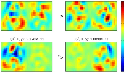
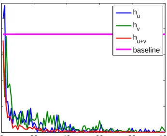
examples; lower row: negative examples. . . 43 2.4 The heatmap of two randomly initialized weight vectorsu,v(upper row) and

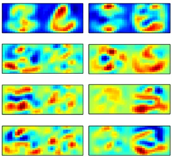
u∗,v∗ learned with PMD (lower row) on the input space. . . 44 2.5 The heatmaps of u,v in 20 PMC iterations (1st iteration on top). . . 45 2.6 The progress made by the two classifiershu, hv in different PMC iterations. 46

2.7 Refining image search ranking with Multi-class PMC. . . 47 2.8 Comparison of PMC and existing works on recognition accuracy obtained with

300 web images and a varying number of Caltech-256 training examples. . . 48 2.9 Venn diagram on domain adaptation. . . 53 2.10 Comparison of self-training, SEDA and CODA on the relative test-error

re-duction over logistic regression, averaged across all 12 domain adaptation tasks. 66 2.11 Comparison of CODA and existing work on the relative test-error reduction

over logistic regression, averaged across all 12 domain adaptation tasks. . . . 67 2.13 The ratio of the average number of used features between source and target

inputs (2.22), tracked throughout the CODA optimization. The three plots show the same statistic at different amounts of target labels. . . 67 2.12 Comparison of CODA and existing work on the absolute test error under

varying amounts of labeled target data on 12 adaptation tasks. . . 70 3.1 Venn diagram on learning from multiple source domains. . . 74

(7)

3.2 Comparison of mSDA and existing works across all twelve domain adaptation task in the small Amazon review dataset. . . 87 3.3 Transfer ratio and training times on the small (left) and full (right) Amazon

Benchmark data. Results are averaged across the twelve and 380 domain adaptation tasks in the respective data sets (5,000 features). . . 87 3.4 Left: Transfer ratio as a function of the input dimensionality (terms are picked

in decreasing order of their frequency). Right: Besides domain adaptation, mSDA also helps in domainrecognition tasks. . . 88 3.5 Venn diagram on learning from corrupted data. . . 94 3.6 Graphical model interpretation of marginalized corrupted features. . . 106 3.7 Classification errors of MCF predictors using blankout corruption – as a

func-tion of the blankout corrupfunc-tion level q – on all data sets for l2-regularized

quadratic, exponential, and quadratic loss functions. The case of MCF with blankout corruption and q= 0 corresponds to a standard l2-regularized

clas-sifier. Figure best viewed in color. . . 110 3.8 The performance of standard and MCF classifiers with blankout and Poisson

corruption models as a function of training set size on the Dmoz and Reuters data sets. Both the standard and MCF predictors employ l2-regularization.

Figure best viewed in color. . . 112 3.9 Comparison between MCF and explicitly adding corrupted examples to the

training set (for quadratic loss) on the Amazon (books) data using blank-out corruption. Training with MCF is equivalent to using infinitely many corrupted copies of the training data. . . 113 3.10 Evaluation on the “Nightmare at test-time” scenario. Classification errors

of standard and MCF predictors with a blankout corruption model – trained using three different losses – and of FDROP [67] on the MNIST data set using the “nightmare at test time” scenario. Classification errors are represented on the y-axis, whereas the amount of features that are deleted out at test time is represented on the x-axis. The images of the digit illustrate the amount of feature deletions applied on the digit images that are used as test data. Figure best viewed in color. . . 115 3.11 Venn diagram on learning with partial supervision. . . 119 3.12 Sample images with associated tags from the Espgame dataset. . . 120 3.13 Schematic illustration of FastTag. During training two linear mappingsBand

W are learned and co-regularized to predict similar results. At testing time, a simple linear mapping x_→Wx predicts tags from image features. . . 124 3.14 Predicted keywords using FastTag for sample images in the Espgame dataset. 129 3.15 Comparison of FastTag and existing work in terms of F1 score vs. training

time on the Corel5K, Espgame and IAPRTC-12 dataset. . . 132 3.16 Comparison of FastTag and existing work at different levels of tag sparsity. . 134

(8)

List of Tables

2.1 Comparison of PMC and existing work on the paired handwritten digit dataset. 43 2.2 Statistics of the Amazon review dataset [19]. . . 64 3.1 Statistics of the large and small set of the Amazon review dataset [19]. . . . 84 3.2 The probability density function (PDF), mean and variance of corrupting

distributions of interest. . . 101 3.3 Moment-generating functions (MGFs) of corrupting distributions of interest. 103 3.4 Comparison of MCF andl2-regularization on classification errors obtained on

the CIFAR-10 data set with simple spatial-pyramid bag-of-visual-word features.114 3.5 Comparison of FastTag and existing work on the Corel5K dataset. . . 131 3.6 Comparison of FastTag and existing work on the Espgame and IAPRTC-12

(9)

Acknowledgments

My utmost gratitude goes to my advisor Kilian Q. Weinberger. Without him, none of the work described in this dissertation would have been possible. Kilian has been an amazing advisor, who introduced me into the field, inspired me with invaluable insights and guided me through the entire course to finish this dissertation. He always makes himself available to discuss ideas and to provide extremely helpful feedbacks. His enthusiasm for research and encouragement have kept me continuing my work.

I would like to thank John Blitzer, Olivier Chapelle, Laurens van der Maaten and Fei Sha for their invaluable input and contributions to these works. John also kindly served as my external committee member and provided me with very useful comments. Every meeting with Olivier and Fei brings me new knowledge about the field. Laurens has led the effort for the work I presented in Section 3.2. I would also like to thank my other committee members John Cunningham, Tao Ju, Robert Pless and Bill Smart for their helpful suggestions. I would like to thank Yixin Chen for his support during the first few years of my PhD study. Further, I would like to thank Jian-Tao Sun, Prabhakar Krishnamurthy and Alice Zheng for providing me with great opportunities to intern at Microsoft Research Asia, Yahoo! Labs and Microsoft Research.

I would like to thank my group members, Eddie Xu, Stephen Tyree, Dor Kedem and Matt Kusner for collaborating on projects, bouncing off ideas, and generously taking time to help with my writings and talks. I will miss the time we spent together working toward the same deadline. I would also like to thank all my friends in St. Louis, who have made the past six years some of the most memorable years in my life.

I would like to thank my parents and grandparents for their unconditional love and support, having faith in me when I have doubts. I am also very thankful to my uncle who first encouraged me to pursue postgraduate study.

(10)

With great love, I thank my husband Zijian Guo for sharing with me all the joys and supporting me through the rough time whole-heartedly.

Minmin Chen

Washington University in Saint Louis

(11)

(12)

ABSTRACT OF THE DISSERTATION

Learning with Single View Co-training and Marginalized Dropout by

Minmin Chen

Doctor of Philosophy in Computer Science Washington University in St. Louis, May 2013

Research Advisor: Kilian Q. Weinberger

The generalization properties of most existing machine learning techniques are predicated on the assumptions that 1) a sufficiently large quantity of training data is available; 2) the training and testing data come from some common distribution. Although these assumptions are often met in practice, there are also many scenarios in which training data from the relevant distribution is insufficient. We focus on making use of additional data, which is readily available or can be obtained easily but comes from a different distribution than the testing data, to aid learning.

We present five learning scenarios, depending on how the distribution we used to sample the additional training data differs from the testing distribution: 1) learning with weak supervision; 2) domain adaptation; 3) learning from multiple domains; 4) learning from corrupted data; 5) learning with partial supervision.

We introduce two strategies and manifest them in five ways to cope with the difference between the training and testing distribution. The first strategy, which gives rise to Pseudo

(13)

Multi-view Co-training (PMC) andCo-training for Domain Adaptation (CODA), is inspired by the co-training [23] algorithm for multi-view data. PMC generalizes co-training to the more common single view data and allows us to learn from weakly labeled data retrieved free from the web. CODA integrates PMC with an another feature selection component to address the feature incompatibility between domains for domain adaptation. PMC and CODA are evaluated on a variety of real datasets, and both yield record performance.

The second strategy marginalized dropout leads tomarginalized Stacked Denoising

Autoen-coders (mSDA), Marginalized Corrupted Features (MCF) and FastTag (FastTag). mSDA

diminishes the difference between distributions associated with different domains by learn-ing a new representation through marginalized corruption and reconstruciton. MCF learns from a known distribution which is created by corrupting a small set of training data, and im-proves robustness of learned classifiers by training on “infinitely” many data sampled from the distribution. FastTag applies marginalized dropout to the output of partially labeled data to recover missing labels for multi-label tasks. These three algorithms not only achieve the state-of-art performance in various tasks, but also deliver orders of magnitude speed up at training and testing comparing to competing algorithms.

(14)

Chapter 1 Introduction

Machine learning is a relatively new branch of artificial intelligence, which aims at getting computers to act based on past experience instead of being explicitly programmed. Tom M. Mitchell provided a widely quoted definition of learning from experience as follows:

A computer program is said to learn from experience E with respect to some class of tasks T and performance measureP, if its performance at tasks inT, as measured byP, improves with experience E. [111]

Experience is commonly embodied in the (large amount of) external data inputted to the computer program. Considering the task of spam filtering, where the goal is to distinguish between spam and non-spam messages. To build such a machine, a large amount of email messages are often provided to learn patterns or regularities that can differentiate spam and non-spam messages. After learning, these patterns or regularities are then used to classify new email messages into spam or non-spam folders.

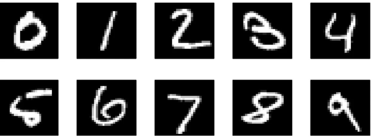
Figure 1.1 illustrates another example of recognizing handwritten digits. The task is non-trivial as handwriting varies greatly. To enable learning, we are provided with a data corpus of handwritten digits. Each input in the corpus is a 28_×28 pixel image, which can be rep-resented as a vector of 784 real numbers. The goal is a build a recognizer so that whenever a new image of handwritten digit comes in, we will be able to produce the identity of the digit 0,_{· · ·} ,9 as the output.

(15)

Figure 1.1: Sample images from the MNIST handwritten digit dataset.

In summary, the goal of machine learning is to automatically extract statistical regularities and patterns presented in a data corpus, and later to act on unseen inputs with the use of these regularities and patterns.

Note that, there is another class of important techniques in machine learning,reinforcement learning, which has a different setup. It deals with the problem of finding suitable actions to take in a given situation in order to maximize a reward, and studies the tradeoff between exploration and exploitation. Instead of being provided with a data corpus beforehand, the learner receives feedback (reward) while acting. However, we are not going to discuss it in this thesis and would like to refer interested readers to [90, 149].

To measure the performance of different learning algorithms, the data corpus is often di-vided into two subsets. One is called the training data, on which the learning takes places. The remaining one is the testing data, on which the prediction and measure of quality are performed.

Note that, a feature extraction stage that preprocess the original raw input into an input vector is often required before any learning or testing can happen. For example, in the case of handwritten digit recognition, typically each image is translated and rescaled so that the digit is centered in a box of fixed size (28_×28 in the example). The gray scale at each pixel of the box is then extracted to form an input vector. The space in which the input vectors lie in is commonly referred to as the feature (or instance) space. Note that the preprocessing of the training and testing inputs has to follow the same protocol. For almost all practical

(16)

applications, the feature extraction stage is equally important as the learning method itself. A good feature extraction stage reduces the noisy variations in the raw input and leads to easier pattern recognition in the learning phrase. However, we will focus on the learning methods in this dissertation.

1.1 Supervised, Unsupervised and Semi-Supervised

Learn-ing

Based upon the types of information that are included in the training data, one can roughly divide different learning methods into three camps: supervised, unsupervised and semi-supervised learning.

1.1.1 Supervised Learning

Let _{X ∈ R}d denote the feature space of dimension d, and _Y the label (or output) space. In supervised learning, the training data is assumed to sampled i.i.d. (independently and identically distributed) from some joint distribution_D on_{X × Y} and comes in in pairs, i.e.,

D = _{(x1, y1),· · · ,(xn, yn)} ⊂ X × Y. Here xi is the input vector and yi is its associated

label (or output). In the example of handwritten digits, the input vector xi corresponds to

the 784 pixel values extracted from the 28_×28 grid, and the label yi corresponds to the

identity of the digit, ranging from 0 to 9. It is assumed that there is an underlying target function f which generates the labels from the inputs, i.e., yi =f(xi). However, the target

function f is usually unknown, and needs to be inferred from the training data. We can further divide the tasks into a classification or aregression one based on the labels. In the the handwritten digit recognition, or the spam filtering task we introduced, the goal is to categorize each input vector into an output from a discrete and finite set. In these cases, we have a classification problem. Examples of classification algorithms includes k-nearest neighbors [47] and support vector machines [156, 135]. When the labels take continuous values, it is a regression task. Examples of regression algorithms include linear regression, kernel regression [64] and gaussian process [125]. Note that there are more complicated tasks

(17)

where structural dependencies exits between the inputs xi’s and the outputs yi’s. In these

cases more specialized algorithms will be required.

Generalization. The output of these learning algorithms can be expressed as a function

h(x) which takes an input vector x and output a prediction ˆy = h(x). In the case of supervised learning, the evaluation of learning quality is well-defined since we can compare the prediction ˆy to the ground truth y. Let us define a binary indicator function

[h(x)₆=y] =

(

0, h(x) =y

1, h(x)₆=y

We can then compute the error of a learner on the training set (the empirical risk) as

D(h) = 1 n n X i=1 [h(xi)6=yi] (1.1)

But we are not really interested in the error on the training set, instead, we want to find a learner which generalizes well to unseen test data. The generalization risk can be expressed as the expected error under the underlying distribution _D,

(h) = E(x,y)∼D[h(x)6=y] (1.2)

However, since the distribution_Dis unknown, we can not explicitly compute it. Fortunately, we can relate the generalization risk of any hypothesis h from a hypothesis class _H to its empirical risk with the help of Vapnik-Chervonenkis theory [156]. For any h _{∈ H}, trained on a set of training data _{(xi, yi)}ni=1 sampled i.i.d. from D, with probability 1−δ,

(h)_≤D(h) + 2 s 2|H|log 2en |H| + log 2 δ n (1.3)

where_|H|denotes the Vapnik-Chervonenkis dimension [156] of the hypothesis class. We can see that the gap between the generalization and empirical error grows inversely with the size of the training data.

In other words, the generalization performance of supervised learning methods are predicated on the condition that a sufficiently large quantity of training data is available for learning.

(18)

1.1.2 Unsupervised Learning

Although extracting the input vectors can often be done very conveniently, acquiring labels turns out to be very expensive for a many tasks. For instance, it takes 2 years to annotate 4,000 sentences in the Penn Chinese Treebank. In annotating phone conversation, 400 hours of annotation time is required for one hour of speech.

Unsupervised learning offers possibilities to circumvent the costly manual annotation. In unsupervised learning, the training data X = _{x1,· · · ,xn} is still assumed to be drawn

i.i.d. from some underlying distribution _D, however, the labels of these inputs are unknown. Common unsupervised learning tasks include: 1) dimensionality reduction; The goal is to project the inputs to a lower-dimensional space where a more meaningful distance interpre-tation or visualization is possible. Examples of dimensionality reduction algorithms include principal component analysis [89], Isomap [151], locally linear embedding [130], Laplacian eigmenmap [8], and maximum variance unfolding [163]. 2) clustering; The goal is to dis-cover similarity between examples and group the inputs into clusters. Examples of clustering algorithms include k-means, and spectral clustering [114]. 3)density estimation; The goal is to infer the underlying distribution that have generated the training data X. Examples of density estimation algorithms include mixture models [107].

Since the inputs given to the learner are unlabeled, generally there is no error or reward signal that can be used to evaluate a potential solution in unsupervised learning. Though for some tasks, such as clustering, it is possible to measure the quality of the solution if some ground truth about the underlying clusters is available.

1.1.3 Semi-Supervised Learning

Semi-supervised learning is halfway between supervised and unsupervised learning. It does not seek to completely eliminate the needs for labels, but resorts to unlabeled data to mini-mize the amount of labeling effort required to achieve good performance.

In semi-supervised learning, the training data contains a relatively small set of input-output pairs drawn from some joint distribution _D, L = _{(x1, y1),· · · ,(xn, yn)} ⊆ X × Y, as well

(19)

as another set of inputs U = _{xn+1,· · · ,xm} drawn i.i.d. from the same distribution. The

labels of the inputs in U are unknown though. The size of the labeled data L is usually much smaller than the unlabeled data U, that is, n m. The goal is to find a hypothesis

h _{∈ H} using both the labeled inputs from L and the unlabeled inputs from U, so that it accurately predicts the labels of test inputs sampled from the same distribution.

Semi-supervised learning algorithms can be roughly divided into four classes based on the different assumptions made in these algorithms: 1) generative models; These models are based on the smoothness assumption of semi-supervised learning. Examples of algorithms in this class include EM algorithms on mixture models [117]. 2) low density separation

models; These models follow the assumption that the decision boundary should lie in a

low-density region. Examples of algorithms in this class include Transductive SVM [88, 38, 143], entropy or information regularization models [150, 71] . 3) manifold-based methods; These models follow the assumption that high-dimensional data lie (roughly) on a low-dimensional manifold. Dimensionality reduction algorithms [89, 151, 130, 8, 163] are performed on all the data, labeled or unlabeled, to find a new representation, and supervised learning is then performed on the new representation using labeled data only. 4)graph-based models; These models are inspired by the cluster assumption: points within the same cluster should be of the same class. Algorithms in this class penalize non-smoothness along the edges of a weighted graph and propagate labels along the edges. Examples of algorithms in this class include graph mincut [24], gaussian random fields and harmonic function method [175], graph kernels [39, 144]. Self-training [168] and co-training [23] are another two prominent semi-supervised learning algorithms. A complete discussion on these work is beyond the scope of this thesis. We refer the readers to [36, 174] for a detailed study on this topic.

1.2 Motivation and Overview

Machine learning has become the tool of choice for many applications. However, successful applications of machine learning often rely on the existence of large quantities of labeled data, which can be difficult to obtain. In recent years, the research community has delved into crowdsourcing as a potential platform for acquiring labels cheaply and at scale [81]. However,

(20)

crowdsourced labels are often very noisy and inconsistent, and obtaining high-quality labels can still be expensive, especially for large-scale datasets.

Unsupervised and semi-supervised learning approaches alleviate the problem. However, most of the algorithms we reviewed in section 1.1.2 and 1.1.3 still assume that 1) the training data, labeled or unlabeled, comes from the same distribution as the testing data 2) the labels are clean and complete. As technology enables data collection at ever increasing scale and speed, nowadays we have access to an enormous amount of data. Unfortunately, not all of these data, in fact, a majority part of these data does not necessarily follow the same distribution as the testing data.

In this dissertation, we focus on making use of additional external data, which comes from a slightly different distribution than the test data, to aid learning. We are concerned with five learning scenarios that differ from classical supervised, unsupervised, or semi-supervised learning, i.e. 1) learning with weak supervision; 2) domain adaptation; 3) learning from multiple domains; 4) learning from dropout distribution; 5) learning with partial supervision. In Chapter 2, we are going to cover the first two scenarios with a common strategy – single view co-training. In Chapter 3, we are going to elaborate our second strategy – marginalized dropout to learn in the remaining three scenarios.

1.2.1 Learning with Weak Supervision

Nowadays, it is possible to obtain large quantities of data for almost any topic or class description with very little human intervention (e.g. through automated image search or wikipedia lookups). For example, we can retrieve hundreds of thousands of images of dif-ferent objects by searching on any of the search engines using the class description of these objects as queries. Typing the keywords “eiffel tower” into Bing returns thousands of images semantically applicable to the concept of eiffel tower. However, not all of the retrieved re-sults are relevant to the query concept. As images are mostly indexed by surrounding texts, the fraction of returned results which are visually relevant to the query concept is usually small. As a result, the distribution of the retrieved images are very different from that of the training/testing data carefully curated by human annotators.

(21)

Figure 1.2 shows sample images from the Caltech256 object recognition benchmark dataset [73] and the top ranked results [11] returned by BingTM _{image search using the class names as}

queries. Each row shows images from one particular object class.

Caltech256 contains over 30,000 images of 256 object categories handpicked and annotated by human annotators. Candidate images are collected from the web following the same protocol we just introduced,i.e., through automated image search. What is different in this case is that a manual cleanup process is implemented afterwards. Annotators are explicitly asked to rule out images that are 1) very cluttered; 2) line drawings; 3) abstract or artistic; 4) not largely occupied by the object. As a result, images within each category are fairly consistent both visually and semantically.

In contrast, the web images appear to be less homogeneous visually due to polysemy, carica-turization, as well as variations in viewpoints. One can observe that: 1) even the top ranked results returned still contain outliers (i.e., images unrelated to the object categoryvisually); For instance, the naked women in the “eiffel tower” category, and the cliff in the “hawksbill” category. They are not completely irrelevant to the query concept itself as a word often has multiple meanings. The image is returned probably because the caption or the text sur-rounding the image describes it as “a women posing like the eiffel tower”. To some extent, it is desirable for a search engine to be able to return a diverse set of results. But the diversity also poses a great challenge for learning. 2) even relevant results in the Bing group are still of noticeable difference to the training images from Caltech256; First, while the Caltech256 benchmark set consists of only real photographs, the Bing retrieved results include cartoon drawings for almost all the seven categories. Second, the hand collected images contain only object of interest, while the Bing counterpart often includes extraneous items, such as people or faces. These image can distract the learning as “people” and “faces” are also valid object categories in the Caltech256 set. 3) Comparing to the human curated images, where the object of interest is in the center, the web images are often taken from very different shooting distances or angles, causing the images to appear less common visually.

In summary, the images returned by Bing search are semantically and visually less coherent than the images from the Caltech256 benchmark set. One can regard the Bing group as a noisy superset of the Caltech256 training data. It contains images which are closely related

(22)

to the object category, but also images which are only remotely connected, or even irrelevant. In this setting, we aims at utilizing the noisy set to assist learning.

Caltech256 Bing

hot air balloon

american flag basketball hoop beer mug boombox eiffel tower hawksbill

Figure 1.2: Sample images from the Caltech-256 object recognition benchmark set [73] and Bing top ranked results [11].

(23)

Notation. We define the setup of learning with weak supervision as follows: let L =

{(x1, y1),· · · ,(xn, yn)} ⊆ X × Y be a small set of input-output pairs drawn from some joint

distribution _D. Let L0 = _{(x1, y1),· · · ,(xm, ym)}, m n be another set of labeled inputs

drawn from a different distribution _D0. The support of _D0 is a superset of the support of the testing distribution _D. The goal is to find a hypothesis h _{∈ H} using both the labeled data from L and L0 to accurately predicts the labels of the testing data drawn from the distribution _D.

Pseudo Multi-view Co-training (PMC) [42]. Section 2.1 describes Pseudo Multi-view Co-training (PMC), an new framework we developed to learn from weak supervision. It is a variant of the co-training [23] algorithm for semi-supervised learning. Similar to Co-training, it cherry-picks the examples which are close to the training data from the noisy labeled set L0 to expand the labeled set L. Different to co-training, which is designed to work with multi-view data, PMC works on the more common single view data. The idea is to automatically divide the features of a single view data set into two mutually exclusive subsets – thereby creating a pseudo-multi-view representation for co-training. Inspired by a theoretical analysis of Balcan et al. [5], the feature division is learned explicitly to satisfy the necessary conditions to enable successful co-training. PMC successfully exploits noisy web search results to improve on the challenging Caltech-256 object recognition task.

1.2.2 Domain Adaptation

The second learning scenario we are interested arises when we have plenty of training data available from some source domain, but are ultimately interested in learning a model that generalizes well to a relatedtarget domain. Re-collecting training data for the target domain is costly, and one often wishes to leverage the data from the source domain, and adapt the learner trained on the source inputs to the new target domain. The challenge is that the data distribution of the target domain often differs from that of the source domain.

The needs to adapt between domains surface everyday as personalization becomes preva-lent, not only in web applications such as personalized news or ads, but also in education, healthcare and television, etc. As an example, spam filters can be trained on some public collection of spam and non-spam emails. However, when applied to an individual user’s

(24)

I read 2-3 books a week, and this is without doubt my

favorite of this year. A beautiful novel by Afghan-American Khaled Hosseini that rans among the best-written and provocative stories of the year so far. This unusually

eloquent story is also about the fragile relationship …

This unit makes the best coffee I've had in a home. It is my

favorite unit. It makes excellent and HOT coffee. The carafe is solidly constructed and fits securely in squared body. The timer is easy to program, as is the clock ...

Figure 1.3: Sample review from the book (left) and kitchen appliance (right) domain of the Amazon review benchmark set [19].

inbox, we may want to “personalize” the spam filter, i.e., adapt it to fit the user’s own distribution of emails in order to achieve better performance. Shift of domain is common in natural language processing as well. In general, labeled data for tasks like part-of-speech tagging, parsing, or information extraction are drawn from a limited set of document types and genres in a given language because of availability, cost, and project goals. However, applications for the trained systems often involve somewhat different document types and genres [52]. For example, most of the labeling were performed on text from news articles (in particular, the Wall Street Journal), which uses a very specialized set of languages. Labeled data from this domain can be a poor match to be used as training examples for other do-mains, such as biomedical texts, mails or meeting transcripts, etc. Another example arises in the vision community. The changes in camera, image resolution, lighting, background, viewpoint, and post-processing cause substantial distribution shift for vision data [132]. For example, there are a large number of readily categorized inventory images online (from Ama-zon, Ebay, etc.), which can be useful for object recognition tasks. However, inventory images are mostly captured in a much more controlled manner, and look very different from the ones taken in real world surroundings. As a result, directly porting a learner trained on thesource

domain (inventory images) to thetarget domain (real life images) often leads to degenerated performance.

(25)

If the data distribution from thesource andtarget domain differs vastly, then it is hopeless to generalize from one to another. Nevertheless, adaptation is possible when the two domains are related,e.g., the two distributions share supports, or the supports of the two distributions overlap. Figure 1.3 shows two sample reviews from the Amazon review benchmark set [19], one from the “books” domain (left), and the other from the “kitchen appliances” domain (right). We highlight the sentiment words that are shared across domains in green, and the ones that are specific to different domains in blue (source) and red (target) respectively. One can see that very different vocabularies are used to express the same kind of opinion (in this case, positive sentiment) about different products. People use “well-written” and “eloquent” when recommending books. On the other hand, “solidly constructed” and “easy to program” are used as strong indicators of positive view about coffee makers. Fortunately, there are also words shared across both products, like “best”, “favorite”. These features are invariant across different domains, and will be used to bridge the two distributions.

Notation. We formalize the setup in domain adaptation as follows: denote as LS = {(x1, y1),· · · ,(xnS, ynS)} ⊆ X × Y the set of labeled data drawn from some source distri-bution _DS, LT = {(x1, y1),· · · ,(xnT, ynT)} ⊆ X × Y a small set of labeled data sampled from the target distribution _DT. Let UT = {xnT+1,· · · ,xmT}, mT nT be another set of unlabeled data drawn i.i.d. from the same target distribution. Note that,LT could be empty

in some cases, i.e., we only have access to unlabeled data from the target domain. The goal is to find a hypothesish_{∈ H} using both the labeled data from LS, the labeled and data LT

and unlabeled data UT from the target domain, so that it accurately predicts the labels of

the testing data drawn from the target distribution_DT.

Co-training for Domain Adaptation (CODA) [41]. Section 2.2 describes Co-training for Domain Adaptation (CODA), an algorithm we developed to adapt from a single source

domain. CODA is a variant of the Pseudo Multi-view Co-training (PMC) algorithm we introduced for learning with weak supervision. It slowly adapts the training set from the source distribution to the target, both data-wise and feature-wise. To shift the distribution of the training data from source to target, CODA gradually add inputs from the target domain to the training set using co-training. Meanwhile, it includes a feature selection component to shift the features used by the model from source-heavy to target-heavy. Combining these two strategies, CODA significantly outperforms existing algorithms on a standard domain adaptation benchmark set [19].

(26)

1.2.3 Learning from Multiple Domains

Most existing work on domain adaptation has been focused on the one source and one target scenario. Here we generalize to the cases when there are multiple source domains, each associated with a different distribution. Glorot et al. [69] demonstrated that learning a shared representation using data from all the available domains leads to better performance than learning on a single source and target domain.

Notation. We formalize the setup in learning with multiple domains as follows: Let K

denote the number of source domains available. Each source domain is associated with a distribution _DSj, j = 1,· · · , K, from which we can sample a set of labeled inputs LSj =

{(x1, y1),· · · ,(xn_Sj, yn_Sj)} and a set of unlabeled inputs USj = {x1,· · · ,xm_Sj}. Note that, it is possible that we only have access to unlabeled data for some source domains. Same as before, denote as LT = {(x1, y1),· · · ,(xnT, ynT)} ⊆ X × Y a small set of labeled data sampled from the target distribution _DT. Let UT ={xnT+1,· · · ,xmT}, mT nT be another set of unlabeled data drawn i.i.d. from the same target distribution. Note that, LT could be

empty in some cases. Again, the goal is to find a hypothesis h_{∈ H} that works well for the target domain.

marginalized Stacked Denoising Autoencoders (mSDA) [43]. Section 3.1 describes marginalized Stacked Denoising Autoencoders (mSDA), an algorithm we developed to learn from multiple source domains. mSDA is inspired by the Stacked Denoising Autoencoders (SDAs) algorithm Glorot et al. [69] adopted for domain adaptation. Similar to SDAs, mSDAs learn a general data representation through corruption and reconstruction using all the unlabeled data from different domains, and then train a classifier using labeled data on the new representation. Different to SDAs, which employ a nonlinear encoders and decoders to learn the representation, mSDAs use single-layer linear denoising autoencoders as the basic building blocks. Our new formulation has some very desirable optimization properties, such as layer-wise closed form solution and noise marginalization. mSDAs match the record accuracy attained by SDAs while reducing the training time by several orders of magnitude.

(27)

1.2.4 Learning from Corrupted Data

Again here we focus on the scenario when the training data from the relevant distribution is insufficient. However, in this case, we do not assume there is data from a different distribution that is readily available or can be easily obtained. Training on the small set of training data often results in degenerated performance on unseen testing data although the learner has low empirical risk, which is commonly referred to as overfitting. The standard approach to deal with overfitting is through regularization or learning with priors. However, these approaches can be unintuitive for practitioners (such as biologists) as prior knowledge on the model parameters is required to select a proper regularizer or prior. Instead, we explore using feature dropout (or data corruption) to create a distribution with known density function and sample from it more training data to improve the robustness of the learned classifiers. Figure 1.4 shows some of the corrupting distributions we used to create the additional train-ing examples. Feature dropout randomly removes some active features (in this case, pixels or image patches of an image) from each example. Bit-swap noise randomly replaces some active features with another ones, which is extremely useful for text document. Imagine peo-ple switch between synonyms, such as replacing “president” with “obama” in the exampeo-ple. Poisson corruption is also useful for count vectors. As shown in the figure, applying these corruption does not change the output, but produces additional training examples that can capture some of the distribution variation which can not be captured in the original small set of training examples.

Marginalized Corrupted Feature (MCF) [155]. Section 3.2 describes Marginalized Corrupted Features (MCF) regularization, an new learning framework we developed to im-prove generalization when no additional external data is available. MCF is inspired by the marginalized corruption employed in mSDA. It extends the training set with infinitely many artificially generated training examples that are obtained by corrupting the original training data. In other words, instead of approximating the exact statistics of the testing distribution

D with finite data, MCF learns from a slightly modified data distribution _D0 with infinite training data. MCF is practical and efficient for a range of predictors and corruption models. We show empirically on a variety of data sets that MCF classifiers can be trained efficiently, may generalize substantially better to test data, and are also more robust to feature deletion at test time. In contrast to regularization or learning with prior method, learning with MCF

(28)

Definitely a car

Still a car?

(a) object recognition

(b) text classification (c) sentiment analysis

keep 0 amazing 5 ideas 2 value 0 poor 0 ... ... average 1

4 Positive review

Still positive?

0

1

president 1 Obama 0 important 1 game-changing 0 ... ... bill 1 law 0

0

1 Politics

Still politics?

Figure 1.4: Examples of applying (a) feature dropout (blank-out noise); (b) Bit-swap noise; (c) Poisson noise to create examples that look like “real” ones.

is more intuitive as the corrupting is applied to the data itself, and we provides some simple guideline for choosing corrupting distributions.

1.2.5 Learning with Partial Supervision

The last learning scenario we are going to explore is to learn with partial supervision. Ac-quiring clean and complete labels can be time consuming and require domain expertise that few possess. Lately, people have been turning to crowdsourcing as a tool for obtaining labels at scale. However, crowd sourced labels are noisy and notoriously incomplete.

(29)

incomplete user tags

y

visual features full list of relevant tags snow, lake, feet mountain, snow, sky, lake, water, feet, legs, boat, trees

x

Figure 1.5: Sample image with partial tags.

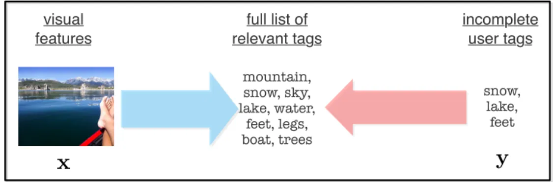
We take automatic image annotation [17, 49, 57, 75, 85, 94, 104] as an example. Given an image, the goal is to annotate it with the complete list of tags that describe all visual features present in the image. Note that it is easy to tag an image with a few of the most prominent visual features, but to obtain the complete list can be quite difficult. The ESP game [162] takes the novel approach of allowing free-form input from the user, which is quick to do, but incentivizes pairs of labelers to match their answers. This results in tag sets with high precision, but without guarantees for high recall; that is, each image may be tagged with only a small set of tags that describe the most obvious visual features.

Figure 1.5 shows an image with a partial list of tags, which prescribes the dominant objects in the image,i.e., snow, lake and feet. Our goal is to infer the full list of relevant tags, which describes all the visual features present in the image, e.g., mountain, snow, sky, lake and water, etc. To be able to tag an image with the full list of tags is important for indexing in searchable image databases such as Flickr, Picassa or Facebook. The full list of tags could also serve as a starting point for image caption.

Notation. We formalize the setup of automatic image annotation with partial tags as follows: let _T = _{ω1,· · · , ωT} denote the dictionary of T possible annotation tags. Let L = _{(x1,y1),· · · ,(xn,yn)} ⊂ Rd × {0,1}T denote the set of training data, where each

vector xi ∈ Rd represents the features extracted from the i-th image and each yi prescribes

the small partial subset of tags that are appropriate for the i-th image. Our goal is to learn a linear function W:_Rd_→T, which maps a test imagexi to its complete tag set.

FastTag. Section 3.3 describes FastTag, an algorithm we developed for image annotation using incomplete user tags. It employs a simple yet effective strategy to cope with overly

(30)

sparse supervision. FastTag learn two linear mappings simultaneously, one to recover the missing labels, and the other one to project the inputs to the predicted labels. These two mappings are co-regularized in a jointly convex loss function, which can be efficiently optimized with closed form updates. The simplicity of the framework allows us to incorporate a variety of image descriptors cheaply and to scale to datasets of a large number of images. FastTag matches the current state-of-the-art in tagging quality, yet reduces the training and testing times by several orders of magnitude on several standard real-world benchmark data sets.

1.2.6 Discussion

Note that there are several other popular learning paradigms that share similar goals as the ones we introduced. For example, active learning [138] seeks to reduce the overall amount of labels required by allowing the learning algorithm to interactively query for new labels. It is hoped that with a smart query strategy, the total number of examples required to learn a concept can be much lower than that would have been required in normal supervised learning.

Multiple instance learning (MIL), originally introduced by Dietterich et al. [55], is highly related to learning with weak or partial supervision. Rather than requiring each instance to be labeled as positive or negative, MIL algorithms take a set of bags that are labeled positive or negative as inputs. Labeling effort is reduced in this case as each bag contains many instances and a single label is assigned to one bag of instances. A bag is labeled negative if all the instances in it are negative, or positive if there is at least one positive instance in the bag. Given a collection of labeled bags, MIL algorithms aim at either 1) inducing a concept that will label individual instances correctly; or 2) labeling bags without inducing the concept.

Multi-task learning (MTL) [30, 59, 58, 165, 37] is a learning framework closely related to domain adaptation. Different from domain adaptation, usually there is only a sin-gle distribution on the observations in multi-task learning. Instead, the target functions

(31)

is to improve the performance of learning algorithms on all the tasks by learning classi-fiers for multiple tasks jointly. It works particularly well when the tasks are related and under-sampled.

1.3 Optimization Background

Optimization plays a very important role in machine learning. Most of the works we are going to include in this dissertation follows a simple scheme, that is formulating the objective as an optimization problem, and then solving with an optimization solver. In this section, we are going to briefly review some of the general optimization techniques used in these works. We will start with the basic first order gradient based method for unconstrained optimization problems, followed with a discussion on the augmented Lagrangian method we employed to solve problems with constraints. Further, we will review the analytical solution for least square problems, and the alternating optimization (block coordinate descent) method we applied to transform an optimization problem into two least square problems so that each one of them can be solved analytically.

1.3.1 Gradient-based Method for Unconstrained Optimization

First, we are going to introduce several gradient-based optimization techniques for uncon-strained problems:

min

x∈Rnf(x) (1.4)

For most of the analysis, we assumed that f is a continuously differentiable function. Note that in our algorithms, there are a few optimization problems which have non-differentiable objective functions, they are either handled with a differentiable approximation or by resort-ing to sub-gradient methods [26].

We will start with a brief discussion of the necessary and sufficient conditions for an optimal solution, which offers important insight on several of the optimization solvers we are going to introduce.

(32)

Proposition 1.1. (Necessary Optimality Condition) Letx∗ be an unconstrained local

minimum of f :_Rn _{→ R}_{, and assume that} _f _{is continuously differentiable in an open set} _S

containing x∗, then

∇f(x∗) = 0 (1.5)

If in addition f is twice continuously differentiable within S, then ∇2

f(x∗) :positive semidefinite. (1.6)

Proposition 1.2. (Sufficient Optimality Condition) Let f :_Rn_{→ R} be twice contin-uously differentiable in an open set S. Suppose x∗ _∈S satisfies the conditions that

∇f(x∗) = 0, _∇2f(x∗) :positive semidefinite. (1.7)

Then, x∗ is a strict unconstrained local minimum of f.

We are going to skip the proofs, and refer interested readers to [13].

The first class of methods we are going to review follow a simple iterative descent idea. In other words, they start from some initial point x0 and successively generate x1,x2,· · · as

xk+1 =xk+αkdk, k= 0,1,· · · (1.8)

such that the objective function f is decreased at each iteration. The process stops when the optimality conditions are satisfied. Here the scalar αk is commonly referred to as the

stepsize and dk ∈ Rn as the descent direction.

Descent direction. The class of methods is widely referred to as gradient based method as the descent direction is chosen to be of the opposite direction as the gradient so that the loss can decrease at each iteration. In other words,

∇f(xk)>dk <0. (1.9)

There are many directions that satisfy the condition. Two widely used descent directions lead to the two classes of popular gradient based methods, the steepest descent method,

(33)

and the newton’s method. For steepest descent methods, the descent direction is the right opposite of the gradient direction, that is,

dk =−∇f(xk) ⇒ xk+1 =xk−αk∇f(xk) (1.10)

For newton’s methods, the descent direction is set so that gradient of the second order taylor expansion of f(xk+1) reaches zero,i.e.,

dk=−(∇2f(xk))−1∇f(xk) ⇒ xk+1 =xk−αk(∇2f(xk))−1∇f(xk) (1.11)

Stepsize. Many different strategies have been proposed to set the stepsize as well. For example, the constant stepsize method simply sets αk = s, where s is a small constant.

Though a simple approach, it runs into problems when the constant is either too large (leading to divergence) or too small (slow convergence). The diminishing stepsize method starts with a relatively large step size and decreases the stepsize at each iteration. Some special care has to be taken to ensure sufficient decrease in the loss at each iteration in this case. The exact minimization or limited minimization rules choose the stepsize by solving another optimization problem to minimize the loss f(xK+1) w.r.t the step size αk. Several

line search rules were also proposed, such as the Armijo rule, which finds the largest step size possible with a sufficient decrease in the loss by successive stepsize reduction.

Convergence. If the descent direction is gradient related, then convergence to a station-ary point (zero derivative) is guaranteed for methods using the exact minimization, limited minimization or the Armijo line search rule for general function classes. For constant or di-minishing stepsize method, Liptchitz continuity needs to be further enforced on the objective function to guarantee convergence.

Conjugate Gradient Method

In this section, we are going to explain the Polack-Ribiere flavor of conjugate gradient method [122] in more detail. It is employed in a optimization package 1 _{used in several}

of our algorithms. Conjugate gradient methods is a a class of optimization techniques that

(34)

Figure 1.6: Comparison of conjugate gradient descent (red) and steepest descent with line minimization in terms of convergence rate.

is between steepest descent, which is known to have slow convergence rate, and newton’s method, which has a big overhead for computing and storing the hessian matrix for large problems.

Many loss functions can be roughly approximated as a quadratic form near the local min-ima [13],

f(x) = 1 2x

>

Ax₋x>b+c (1.12)

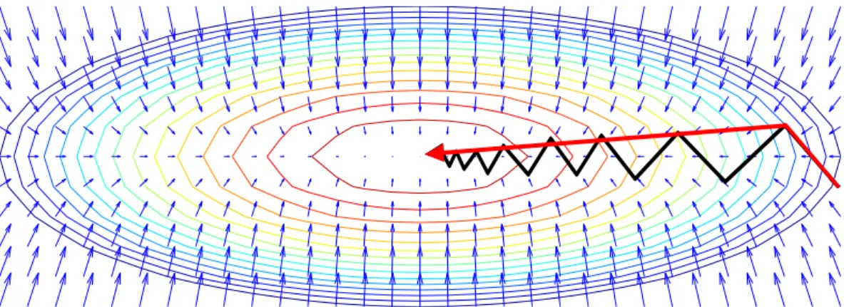
Figure 1.6 compares the convergence rate of steepest descent method (black) and conjugate gradient method (red) when minimizing such a quadratic function. The contour of the objective function is shown in different colors, with the minimum at the bottom center of the narrow “valley”. The plot also depicts the gradients at different point with blue arrows. In the two-dimensional case, one might have hoped that the gradient descent will arrive at the minimum in two steps, where the first step takes you to the bottom of the valley, and the second step directly down to the center. Steepest descent method instead, makes many small steps following the gradient directions. It has a very slow convergence rate, repeatedly searching in the same directions, even when the loss is a perfectly quadratic function. The reason is that with the line minimization rule, the gradients at two consecutive iterations are perpendicular to each other. In other words, you are making a right turn at each iteration, which are not likely to take you to minimum unless matrix A is an identity matrix.

(35)

Algorithm 1.1 Conjugate Gradient Method. 1: Initialization: x0 =0, g0 =−∇f(x0),d0 =g0 2: for k = 0 to n₋1 do 3: αk= g>_kgk d>_iAdi 4: xk+1 =xk+αkdk 5: gk+1 =gk−αkAdk 6: βk+1 = (gk+1−gk)>gk+1 gkgk 7: dk+1 =gk+1+βk+1dk 8: end for

Conjugate gradient method, on the other hand, can solve the problem with at most n

iterations, wheren is the number of variables in x. For the example we plot in figure 1.6, at most 2 steps are required, as depicted in the red arrow. Given a positive definite matrix A, a set of nonzero vectors d0,· · · ,dk is conjugate (A-orthogonal), if

d>_i Adj = 0, ∀i and j such that i6=j. (1.13)

The conjugate directions are linearly independent, therefore a set of n conjugate directions will span the n dimensional space where the minimum x∗ lies in. If we set the update rule as

xk+1 =xk+αkdk

where d0 =−∇f(x0), and dk is conjugate to d0,· · · ,dk−1, and find the stepsizeαk by line

minimization rule, then we can also prove that xk+1 = arg min

x∈Mkf(x) (1.14)

whereMk is the subspace spanned byd0,· · · ,dk. Please refer to [13] page 132 for the proof.

Therefore, at iteration n, we would have found the minimum, xn = arg minx∈Rnf(x)≡x∗. Algorithm 1.1 shows the pseudocode for the conjugate gradient method.

(36)

1.3.2 Augmented Lagrangian Method for Constrained

Optimiza-tion

Some of our problem formulations involve constraints. In this section, we are going to briefly review the augmented Lagrangian method for constrained optimization problem of the following form:

min

x f(x) (1.15)

subject to hi(x) = 0, i= 1,· · · , m gj(x)≤0, j = 1,· · · , r

where the objective function f : _Rn _{→ R}_{, the equality constraints} _h

i : Rn → R, i =

1,_{· · ·} , m, and the inequality constraints gi : Rn → R, j = 1,· · · , r are continuously

differ-entiable.

The constrained optimization problem can be well approximated with an unconstrained optimization of the augmented lagrangian function

min x,z Lc(x,z, λ, µ) =f(x) + m X i=1 n λihi(x) + c 2h 2 i(x) o (1.16) + r X j=1 n µj(gj(x) +zj2) + c 2(gj(x) +z 2 j) 2o

provided that either:

1) λ and µ are close to the Lagrangian multipliers; or 2) The penalty parameter c is large.

Herez2

j, j = 1,· · · , rare the additional variables introduced to handle inequality constraints.

There are several other popular techniques for constrained optimization. For example, the gradient projection method [127] is widely used in problems involves constraints of convex set. It adds to the steepest descent method for unconstrained optimization an additional projection step to project the search direction to the feasible set. However, in order for

(37)

these methods to make practical sense, it s necessary that the projection operation is fairly simple, which in turn means that the constraints can only take simple structure, such as bounded or linear constraints. (In)exact Penalty method is another alternative. It follows the same philosophy of augmented Lagrangian method, that is, to transform a constrained problem into an unconstrained one, and then solve with techniques we introduced in previous section. It adds any violation in the constraints as additional penalty terms to the objective function. The problem with penalty method is that in order to recover a feasible solution to the original constrained problem, the penalty factors cfor each active constraints have to go to infinity. As c increases, the condition number of the Hessian matrix increases as well, causing the unconstrained formulation to become difficult to solve.

The advantage of augmented Lagrangian method lies in the fact that it is workable even if the penalty factor c is not increased to _∞, thus alleviates the ill-conditioning problem and is in general more reliable then penalty method.

update rule. A good heuristic for updating the penalty factorcis to start with a relatively small value c0 and increase it slightly whenever the constraints are violated. The Lagrangin multipliers are updated as

λk_i+1 =λk_i +ckhi(xk) µkj+1 =µ k

j +ckmax(0, gj(xk, µk, ck)) (1.17)

In our experiments, we found that it is important to roughly tune the initial penalty factor

c0 at some small values so that the augmented unconstrained problem is solvable. Starting

from a too large penalty factor often results in ill-conditioning in the later iterations.

1.3.3 Least-Squares Problem

In this section, we are going to review the least-squares problem which serves as building blocks for a couple of our algorithms. Least-squares is arguably the most well known subclass of convex optimization problems. A least-squares problem is unconstrained, and it take an objective which is a sum of squared residuals of the forma>x₋b,

min x∈Rd f(x) = kAx−bk 2 ₌ n X i=1 (a>_i x₋bi)2 (1.18)

(38)

where A_{∈ R}n×d_{, and} _a>

i corresponds to the rows of A. The vector x∈ Rd is the variables

we optimize over.

We can rewrite the objective function in eq. (1.18) as min

x (Ax−b)

>

(Ax₋b)

= x>A>Ax₋2x>A>b+b>b (1.19)

Take the derivative of (1.19) and set it to zero, we have

A>Ax=A>b (1.20)

In other words, solving the least-squares problem is equivalent to solve the system of linear equations in (1.21), which has closed form solution

x= (A>A)−1A>b. (1.21) Solving the least-squares problem has a time complexity of O(d2_n_{) with a known constant.}

A variety of efficient and reliable implementations, such as gaussian elimination method, for solving the linear system of equations are available. Running a problem with d= 5,000 and

n= 100,000 on a desktop with dual 6 cores Intel i7 cpus with 2.66Ghz takes seconds. The least-squares problem is the basis for regression analysis, optimal control, and many parameter estimation and data fitting methods [25]. It can be further generalized to slightly different formats without breaking the closed form solution. For example, we can include different weights for different rows of A, which corresponds to having different costs for different examples in the regression analysis or data fitting.

min x fω(x) = n X i=1 ωi(a>i x−bi)2 (1.22)

where the weightsω1,_{· · ·} , ωnare non-negative. Let Ω = [ωi]_iidenote a diagonal matrix with

the weightsωi’s on the diagonal, we can then rewrite the weighted version of the least-squares

problem as

min

x fω(x) = (Ax−b)

>

(39)

which has analytical solution as x= (A>ΩA)−1_A>_Ωb.

We can also add additional terms that regularize the variables x to the objective function. For example, when a positive multiple of the sum of squares of the variables are added, we have min x fλ(x) = n X i=1 (a>_i x₋bi)2+λkxk2. (1.24)

where λ is a positive factor penalizing large values in x. The new objective function is commonly referred to as ridge regression. Different regularization reduces to Maximum likelihood estimation of the variables x with different priors. For example, ridge regression corresponds to estimation of x with a gaussian prior; and L1 regularization corresponds to

Laplace prior.

Note that the closed form solution no longer stands in theL1 regularization case. However,

with the introduction of some auxiliary variables, we can solve the problem within a few iterations, where at each iteration an analytical solution is available. We refer interested readers to [25].

1.3.4 Block Coordinate descent (Alternating Optimization)

Another optimization technique we used quite often in our algorithms is the (block) coordi-nate descent method, also known as the alternating optimization. It partitions the variables of the optimization problem x _{∈ R}n _{into several exclusive subsets} _x _{= (x}

(1);· · · ;x(t)),

where x(i) ∈ Rni, satisfying Pt

i=1ni = n. It minimizes the objective function f(x) jointly

over all the variables in x by iteratively carrying out alternating restricted minimization over each subset of variables x(1);· · · ;x(t). In other words, given the current iterate xk =

(xk₍₁₎;_{· · ·} ;xk₍_i₋₁₎;xk₍_i₎;xk₍_i₊₁₎;_{· · ·} ;xk₍_t₎), it generates the next iteratexk+1 as (x₍₁₎k ;_{· · ·} ;xk₍_i₋₁₎;x₍k_i+1₎ ;xk₍_i₊₁₎;_{· · ·} ;xk₍_t₎), where xk₍_i+1₎ = arg min z∈Rnif(x k (1);· · · ;xk(i−1);z;xk(i+1);· · · ;xk(t)) (1.25)

(40)

That is, the variables from all the subsets except subsetiis clamped to the best values found in previous iterations, and the cost function is minimized w.r.t each of the block coordinates xk

(i). The same process is repeated for every block in cyclic order until convergence. The

method is extremely useful if the minimization problem we have in eq. (1.25) is substantially easier than jointly minimizing the loss over all the variables at once. Note that, this approach can get stuck at some local minimum. But it converges to the global minima if the cost function is jointly convex over all the coordinates.

(41)

Chapter 2 Single View Co-training

In this chapter, we are going to explicate our first strategy, single view co-training, for learning with weak supervision or domain adaptation. The co-training algorithm of Blum and Mitchell [23] was originally designed for multi-view data. Section 2.1 details Pseudo

Multi-view Co-training (PMC). PMC generalizes co-training to the more common single

view data with an automatic feature decomposition scheme. The rote learning procedure employed in co-training is a natural fit to learn from weakly labeled data, by cherry-picking the instances that resemble the training examples. We demonstrate on challenging tasks that PMC improves the generalization performance substantially with the help of weakly la-beled data. Section 2.2 detailsCo-training for Domain Adaptation (CODA). CODA adds to PMC another feature selection component to address the missing feature problem in domain adaptation. Combining these two components, CODA is able to slowly adapt the training set from source to target distribution, both data-wise and feature-wise. CODA significantly out-performs the state-of-the-art on the 12-domain benchmark data set of Blitzer et al. [19]. Indeed, over a wide range (65 of 84 comparisons) of target supervision CODA achieves the best performance.

2.1 Pseudo Multi-view Co-training

In this section, we present Pseudo Multi-view Co-training (PMC). PMC is a variant of the Co-training algorithm [23] for multi-view data. In co-training, one trains two classifiers, one on each view, that teach each other with the most confident predictions of the unlabeled data. PMC extends co-training to learning scenarios without an explicit multi-view representation.

(42)

Based on a theoretical analysis of Balcan et al. [5], we introduce a novel algorithm that splits the feature space during learning, explicitly to encourage co-training to be successful. We demonstrate the efficacy of our proposed method in a weakly-supervised setting on the challenging Caltech-256 object recognition task, where we improve significantly over previous results [11] in almost all training-set size settings.

The section is organized as follows. Section 2.1.2 recaps the setup in learning with weak supervision. Section 2.1.3 describes the original co-training algorithm and explains why it is particularly suitable for learning on weakly-labeled data. We survey several theoretical work on relaxing the assumptions in co-training and related work on generalizing co-training to single view data. Section 2.1.4 details the PMC algorithm itself. The algorithm is based on the theoretical work of Balcan et al. [5]. Different from most of the previous approaches, which decompose the feature space in a preprocessing step, we learn the feature decompo-sition along with the two classifiers, explicitly to satisfy the conditions for co-training to succeed. Section 2.1.5 extends the framework to multi-class settings. In Section 2.1.6, we report the performance of PMC on the Caltech-256 object recognition task, using images retrieved from BingTMas weakly labeled data.

2.1.1 Introduction

Co-training [23] is an approach to semi-supervised learning [36, 174] which assumes that the available data is represented with two views. In its original formulation, these two views must satisfy two conditions: 1) each one is sufficient to train a low-error classifier and 2) both are class-conditionally independent. Given a datasets of two such views (representations), co-training trains two classifiers, one on each view. It then utilizes unlabeled data by adding the most confident predictions of each classifier to the training set of the other classifier – effectively letting the classifiers “teach each other”. Blum and Mitchell [23] show drastic improvements on data sets where the multi-view assumptions naturally hold. Co-training and its variants have been applied to many applications across computer science and beyond [45, 66, 116, 98, 27, 33].

However in many learning scenarios, the available data does not originate from two explicitly different sources. For example, in the MNIST handwritten digit dataset we introduced in

Learning with Single View Co-training and Marginalized Dropout

Washington University in St. Louis

Washington University Open Scholarship

Learning with Single View Co-training and

Marginalized Dropout

Minmin Chen

copyright by

Minmin Chen

Contents

List of Figures

List of Tables

Acknowledgments

Minmin Chen

Chapter 1

Introduction

1.1

Supervised, Unsupervised and Semi-Supervised

Learn-ing

1.1.1

Supervised Learning

1.1.2

Unsupervised Learning

1.1.3

Semi-Supervised Learning

1.2

Motivation and Overview

1.2.1

Learning with Weak Supervision

1.2.2

Domain Adaptation

1.2.3

Learning from Multiple Domains

1.2.4

Learning from Corrupted Data

Definitely a car

4

Positive review

0

1

0

1

Politics

1.2.5

Learning with Partial Supervision

y

x

1.2.6

Discussion

1.3

Optimization Background

1.3.1

Gradient-based Method for Unconstrained Optimization

1.3.2

Augmented Lagrangian Method for Constrained

Optimiza-tion

1.3.3

Least-Squares Problem

1.3.4

Block Coordinate descent (Alternating Optimization)

Chapter 2

Single View Co-training

2.1

Pseudo Multi-view Co-training

2.1.1

Introduction